Influence of distinct social contexts of long-term care facilities on the dynamics of spread of COVID-19 under predefine epidemiological scenarios

2.1 Model description

In our model, we consider a city where we subdivide the population into three categories: individuals of the community that do not visit LTCF (Q), individuals from the community who visit a long-term care (T), and the LTCF residents (P). We refer to the members of Q and T population to be non-mobile and mobile individuals, respectively. The third group in our model includes LTCF residents (P) who will be referred to as senior members. The members of the sub-population of T are expected to interact with both sub-populations Q and P, respectively. Besides, disease can also be passed on through interaction within each sub-group as well (Figure 1).

Figure 1

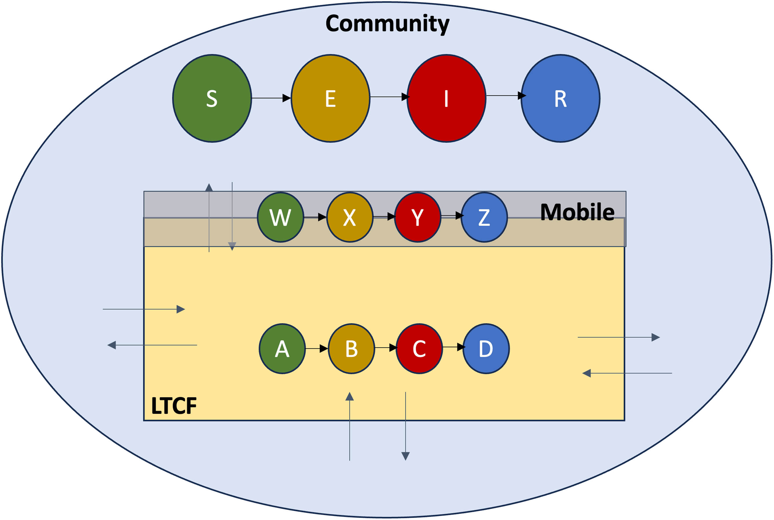
Model dynamics containing three sub-groups: non-mobile, mobile, and old-age home population.

Within each of the sub-groups, we use an S-E-I-R type model that denotes the respective susceptible, exposed (asymptomatic), infectious (symptomatic), and recovered. For our model, the Q sub-population is modeled using S , E , I , and R to denote the respective epidemiological states with total population Q = S + E + I + R , the T sub-population model using W , X , Y , and Z compartments with total population T = W + X + Y + Z , and the older long-term facility group P using the compartments A , B , C , and D with total population P = A + B + C + D . Next, we describe the compartmental models for the three sub-populations defined in Table 1.

Let θ 1 , θ 2 , and θ 3 be the average number of contacts of Q, T, and P per unit time, respectively. Denoting NM to be the non-mobile community members, M-NV and M-V to be mobile community members that either do not visit or visit a LTCF, respectively, and LCO to be local senior residents from the LTCF, we can summarize their contacts via Table 2.

Let τ denote the fraction of mobile youth that visit a LTCF and ω = ( 1 − τ ) be the fraction of mobile youth that are in community. We can then describe the mixing patterns of individuals during the various interactions using appropriate mixing probabilities. We also assume that γ be the fraction of contacts that are reduced due to isolation in the LTCF. If individuals mix according to the proportional mixing scheme [9,11], then these mixing probabilities are defined and given as follows (Table 3):

• P ˜ S X is the mixing probability between non-mobile and mobile youth in the community;

• P ˜ S E is the mixing probability between non-mobile youth within their sub-group;

• P ¯ W X is the mixing probability between mobile youth within their sub-group;

• P ¯ W E is the mixing probability between mobile and non-mobile youth in the community;

• P ¯ W C is the mixing probability between the mobile youth that visit a LTCF and old-age members there;

• P ˆ A X is the mixing probability between old-age members at the LTCF with the mobile youth from the community that visit them;

• P ˆ A B is the mixing probability between old-age members at the LTCF with other exposed old-age members from the facility.

• P ˆ A C is the mixing probability between old-age members at the LTCF with other infected old-age members from the facility.

Note that the mixing probabilities satisfy the following identities:

Let f Q , f T , and f P be defined as the efficacy of the face mask worn by each sub-group and denote the proportion of people that uses face masks effectively. Also, let f ¯ i = 1 − f i for i = Q , T , P denote the proportion that do not use face masks effectively. Note that f P ≫ f Q and f P ≫ f T as well as θ 3 ≪ θ 1 , θ 3 ≪ θ 2 assuming that the senior members in the LTCF will adhere to policies on face masks and social distancing much more than the youth. We also assume that old-age population does not have the ability to self-heal and disease-related death d 2 is higher than the average mortality rate d 1 .

The governing differential equations for the non-mobile population system can then be described by:

The governing differential equations for the mobile (to old-age homes) population system can then be described by:

The governing differential equations for the old-age home population system can then be described by:

In these model equations, the total population corresponding to the non-mobile youth is Q = S + E + I + R , corresponding to mobile youth, which is T = W + X + Y + Z , and corresponding to old-age members at the LTCF is P = A + B + C + D .

Parameters that are used and their definitions are given in Table 4.

3.1 Basic reproduction number

Reproductive number plays an important role in determining the dynamics of spread of a disease. We use here a general approach called the next-generation matrix approach [10,12,17] to find the basic reproduction number ℛ 0 . Given that the infectious states: E , X , B , I , Y , and C in equations (1)–(12), we create a vector ℱ that represents the new infections flowing only into the exposed compartments given by:

where

Along with ℱ , we also consider V , which denotes the outflow from the infectious compartments in equations (1)–(12), which is given by:

where α i = α + d i , i = 1 , 2 .

Next, we compute the Jacobian F from ℱ (see (6)), and the Jacobian V from V (see (6)), Using matrices F and V , we compute the next-generation matrix F V − 1 :

Note that ( i , j ) entry of the next-generation matrix F V − 1 is the expected number of secondary infections in compartment i produced by individuals initially in compartment j assuming that the environment seen by the individual remains homogeneous for the duration of its infection. Also, matrix F V − 1 is non-negative and therefore has a non-negative eigenvalue. The basic reproduction number can then be computed as ℛ 0 = ρ ( F V − 1 ) , which is the spectral radius of the matrix. This non-negative eigenvalue is associated with a non-negative eigenvector, which represents the distribution of infected individuals that produces the greatest number ℛ 0 of secondary infections per generation. In order to calculate the eigenvalues of F V − 1 , we consider the characteristic equation:

where λ denotes the eigenvalues of the matrix and I represents the identity matrix. This can be simplified to yield:

The characteristic polynomial therefore is the following equation given by:

where

The basic reproduction number ℛ 0 corresponds to the dominant eigenvalue given by the dominant root of equation (15) given by:

where

where R ^ * = * ϕ and R ˜ * = * α 2

where

Corollary 1. If the adults in the long-term care are fully protected with face-masks ( f P = 1 ), the infection dies out ( ℛ 0 < 1 ) if

where

Corollary 2. If the adults in the long-term care are fully protected with face-masks ( f P = 1 ), the infection dies out ( ℛ 0 < 1 ) if

Corollary 3. If the adults in the long-term care are fully protected with face-masks ( f P = 1 ) as well as the mobile youth are fully protected with face-masks ( f T = 1 ), then infection dies out ( ℛ 0 < 1 ) if

Note that this suggests that

or this yields a restriction on effective face mask efficacy for the non-mobile youth as follows:

4.1 Model implementation on CDC strategies

We consider here five scenarios given by CDC and implement in our model to understand the strategies that work in favor for LTCFs. We estimate the contact rate θ based on the planning scenarios by CDC [14] as follows:

• Scenario 1  [14]:

  • – Lower-bound values for virus transmissibility and disease severity

  • – Lower percentage of transmission prior to onset of symptoms

  • – Lower percentage of infections that never have symptoms and lower contribution of those cases to transmission

  Using the expression of basic reproductive number R 0 from [26], we estimate θ to be 2.88.

• Scenario 2   [14]:

  • – Lower-bound values for virus transmissibility and disease severity

  • – Higher percentage of transmission prior to the onset of symptoms

  • – Higher percentage of infections that never have symptoms and higher contribution of those cases to transmission

  We estimate the contact rate θ to be 3.17 based on the planning Scenario 2 by CDC [14] from [26].

• Scenario 3 [14]:

  • – Upper-bound values for virus transmissibility and disease severity

  • – Lower percentage of transmission prior to onset of symptoms

  • – Lower percentage of infections that never have symptoms and lower contribution of those cases to transmission

  We estimate the contact rate θ to be 4.5 based on the planning Scenario 3 by CDC [14] from [26].

• Scenario 4 [14]:

  • – Upper-bound values for virus transmissibility and disease severity

  • – Higher percentage of transmission prior to onset of symptoms

  • – Higher percentage of infections that never have symptoms and higher contribution of those cases to transmission

  We estimate the contact rate θ to be 4.89 based on the planning Scenario 4 by CDC [14].

• Scenario 5 [14]:

  • – Parameter values for disease severity, viral transmissibility, and pre-symptomatic and asymptomatic disease transmission represent the best estimate, based on the latest surveillance data and scientific knowledge.

  We estimate the contact rate θ to be 3.43 based on the planning Scenario 5 by CDC [14].

For these five scenarios, the values of θ i for i = 1 , 2 , 3 are calculated as follows: θ 2 = 1.5 * θ 1 and θ 3 = 0 . * θ 1 . Note that this satisfies: θ 3 < θ 1 < θ 2 . The definition of CDC scenarios and the corresponding parameter estimates are collected in Tables 5 and 6, respectively.

The baseline case, defined to reflect early COVID-19 outbreak when interventions were yet to be initiated, is also considered in this analysis. The model parameter estimates for the baseline case were obtained from reference [26] and are collected in Table 6.

4.2 Numerical results

Using our model, we simulate the five scenarios given by CDC in Table 5 to understand and compare the dynamics of COVID-19 in LTCFs under different control strategies. We study the model for 30 days (to capture single outbreak burden) for the population of LTCF residents and visitors to the residents and non-visitors based on parameter estimates given in Table 6.

We divide the section into four subcases of the model describing different modeling assumptions on mixing and mortality. For each subcases, we simulate all the five scenarios. The cases are as follows:

1. negligible disease mortality rate, proportional mixing population, and constant total population

2. negligible disease mortality rate, heterogeneous mixing population, and constant total population

3. high disease mortality rate and proportional mixing population

4. high disease mortality rate, heterogeneous mixing population, and variable community population size.

The dynamics of the non-visitors, visitors, and LTCF members for the five CDC scenarios applied after 30 days compared with baseline are shown for proportional mixing without deaths (Figure 2, i.e., Case 1), heterogeneous mixing without deaths (Figure 3, i.e., Case 2), proportional mixing with deaths (Figure 4, i.e., Case 3), and heterogeneous mixing with deaths (Figure 5, i.e., Case 4).

Figure 2

Dynamics of the non-visitors, visitors, and LTCF members for five CDC scenarios applied after 30 days compared with baseline for proportional mixing without deaths.

Figure 3

Dynamics of the non-visitors, visitors, and LTCF members for five CDC scenarios applied after 30 days compared with baseline for heterogeneous mixing without deaths.

Figure 4

Dynamics of the non-visitors, visitors, and LTCF members for five CDC scenarios applied after 30 days compared with baseline for proportional mixing with deaths.

Figure 5

Dynamics of the non-visitors, visitors, and LTCF members for five CDC scenarios applied after 30 days compared with baseline for heterogeneous mixing with deaths.

We observe that heterogeneous mixing population makes epidemic worse as compared to epidemic size in homogeneous mixing population. Moreover, in the heterogeneous mixing population, the epidemic burden is about 100 times more for community members (visitors and non-visitors) than for the LTCF population. That is, under heterogeneous mixing situation, which may occur due to continuous changes in the population behaviors, can create worse epidemic and particularly for long term care residents, with respect to metrics considered in this study.

Strategies 1, 2, and 5 result in almost similar burden and are the best followed by Strategy 3, whereas Strategy 4 is the worst among all the strategies. This statement is true for both homogeneous and heterogeneous mixing population. Figure 6 shows the influence of face masks on ℛ 0 for the five CDC scenarios applied after 30 days compared with baseline simulation. Strategy 1 has the lowest estimated ℛ 0 followed by Strategies 2, 3, 5, and 4. That is, 30-day disease burden is low in the Scenarios 1, 2, and 5 when compared with Scenarios 3 and 4. This is because transmission rate and/or disease severity rate are at lower levels in case of Scenarios 1, 2, and 5. The lower transmission rate results in slower spread of infection in the population, whereas lower disease severity rate results in shorter infectious period. The epidemic occurs faster with high peak in Scenario 4 (followed by Scenario 3) as compared with other scenarios. This is the result of higher estimated rate of reproduction number in these two scenarios.

Figure 6

Influence of face mask on ℛ 0 for five CDC scenarios applied after 30 days compared with baseline.

References

[1] Ajbar, A., Alqahtani, R. T., & Boumaza, M. (2021). Dynamics of an SIR-based COVID-19 model with linear incidence rate, nonlinear removal rate, and public awareness. Frontiers in Physics, 9, 13. doi: 10.3389/fphy.2021.634251. Search in Google Scholar
[2] Akman, O., Chauhan, S., Ghosh, A., Liesman, S., Michael, E., Mubayi, A., …, Tripathi, J. P. (2022). The hard lessons and shifting modeling trends of COVID-19 dynamics: Multiresolution modeling approach. Bulletin of Mathematical Biology, 84, 1–30. 10.1007/s11538-021-00959-4Search in Google Scholar PubMed PubMed Central
[3] Brauer, F. (1990). Models for the spread of universally fatal diseases. Journal of Mathematical Biology, 28(4), 451–462. 10.1007/BF00178328Search in Google Scholar PubMed
[4] Brauer, F. (2005). The Kermack-McKendrick epidemic model revisited. Mathematical Biosciences, 198(2), 119–131. 10.1016/j.mbs.2005.07.006Search in Google Scholar PubMed
[5] Brauer, F. (2006). Some simple epidemic models. Mathematical Biosciences & Engineering, 3(1), 1. 10.3934/mbe.2006.3.1Search in Google Scholar PubMed
[6] Brauer, F. (2008). Age-of-infection and the final size relation. Mathematical Biosciences & Engineering, 5(4), 681. 10.3934/mbe.2008.5.681Search in Google Scholar PubMed
[7] Brauer, F., Castillo-Chavez, C., & Castillo-Chavez, C. (2012). Mathematical models in population biology and epidemiology (Vol. 2, p. 508). New York: Springer. 10.1007/978-1-4614-1686-9Search in Google Scholar
[8] Brauer, F., Castillo-Chavez, C., & Feng, Z. (2019). Mathematical models in epidemiology (Vol. 32). New York: Springer. 10.1007/978-1-4939-9828-9Search in Google Scholar
[9] Busenberg, S., & Castillo-Chavez, C. (1991). A general solution of the problem of mixing of subpopulations and its application to risk-and age-structured epidemic models for the spread of AIDS. Mathematical Medicine and Biology: A Journal of the IMA, 8(1), 1–29. 10.1093/imammb/8.1.1Search in Google Scholar PubMed
[10] Castillo-Chavez, C., Cooke, K., Huang, W., & Levin, S. A. (1989). The role of long periods of infectiousness in the dynamics of acquired immunodeficiency syndrome (AIDS). In: Mathematical Approaches to Problems in Resource Management and Epidemiology (pp. 177–189). Berlin, Heidelberg: Springer. 10.1007/978-3-642-46693-9_14Search in Google Scholar
[11] Castillo-Chavez, C., Song, B., & Zhang, J. (2003). An epidemic model with virtual mass transportation: The case of smallpox in a large city. In: Bioterrorism: Mathematical Modeling Applications in Homeland Security (pp. 173–197). Society for Industrial and Applied Mathematics. Germany: Springer International Publishing Berlin.10.1137/1.9780898717518.ch8Search in Google Scholar
[12] Castillo-Chavez, C., Velasco-Hernandez, J. X., & Fridman, S. (1994). Modeling contact structures in biology. In Frontiers in Mathematical Biology (pp. 454–491). Berlin, Heidelberg: Springer. 10.1007/978-3-642-50124-1_27Search in Google Scholar
[13] CDC COVID-19 Response Team, CDC COVID-19 Response Team, CDC COVID-19 Response Team, Bialek, S., Boundy, E., Bowen, V., Chow, N., Cohn, A., Dowling, N., …, Gierke, R. (2020). Severe outcomes among patients with coronavirus disease 2019 (COVID-19)-?United States, February 12-March 16, 2020. Morbidity and Mortality Weekly Report, 69(12), 343–346. 10.15585/mmwr.mm6912e2Search in Google Scholar PubMed PubMed Central
[14] COVID-19 Pandemic Planning Scenarios, Uniform Resource Locator: https://www.cdc.gov/coronavirus/2019-ncov/hcp/planning-scenarios.html. 2021. Search in Google Scholar
[15] Chidambaram P. (2020). https://www.kff.org/coronavirus-covid-19/issue-brief/state-reporting-of-cases-and-deaths-due-to-covid-19-in-long-term-care-facilities/. Search in Google Scholar
[16] Comas-Herrera, A., Zalakaín, J., Lemmon, E., Henderson, D., Litwin, C., Hsu, A. T., …, Fernández, J. L. (2020). Mortality associated with COVID-19 in care homes: International evidence. Article in LTCcovid.org, International Long-term Care Policy Network, CPEC-LSE, 14. Search in Google Scholar
[17] Diekmann, O., Heesterbeek, J. A. P., & Metz, J. A. (1990). On the definition and the computation of the basic reproduction ratio R 0 in models for infectious diseases in heterogeneous populations. Journal of Mathematical Biology, 28(4), 365–382. 10.1007/BF00178324Search in Google Scholar PubMed
[18] Dora, A. V., Winnett, A., Jatt, L. P., Davar, K., Watanabe, M., Sohn, L., …, Goetz, M. B., (2020). Universal and serial laboratory testing for SARS-CoV-2 at a long-term care skilled nursing facility for veterans-?Los Angeles, California, 2020. Morbidity and Mortality Weekly Report, 69(21), 651. 10.15585/mmwr.mm6921e1Search in Google Scholar PubMed PubMed Central
[19] Kimball, A., Hatfield, K. M., Arons, M., James, A., Taylor, J., Spicer, K., …, Bell, J. M. (2020). Asymptomatic and presymptomatic SARS-CoV-2 infections in residents of a long-term care skilled nursing facility-?King County, Washington, March 2020. Morbidity and Mortality Weekly Report, 69(13), 377. 10.15585/mmwr.mm6913e1Search in Google Scholar PubMed PubMed Central
[20] King County, Update: King County COVID-19 case numbers for March 6, 2020, kingcounty.gov, 2020. Search in Google Scholar
[21] Lauer, S. A., Grantz, K. H., Bi, Q., Jones, F. K., Zheng, Q., Meredith, H. R., …, Lessler, J. (2020). The incubation period of coronavirus disease 2019 (COVID-19) from publicly reported confirmed cases: Estimation and application. Annals of Internal Medicine, 172(9), 577–582. 10.7326/M20-0504Search in Google Scholar PubMed PubMed Central
[22] McMichael, T. M., Currie, D. W., Clark, S., Pogosjans, S., Kay, M., Schwartz, N. G., …, Ferro, J. (2020). Epidemiology of COVID-19 in a long-term care facility in King County, Washington. New England Journal of Medicine, 382(21), 2005–2011. 10.1056/NEJMoa2005412Search in Google Scholar PubMed PubMed Central
[23] Nuño, M., Reichert, T. A., Chowell, G., & Gumel, A. B. (2008). Protecting residential care facilities from pandemic influenza. Proceedings of the National Academy of Sciences, 105(30), 10625–10630. 10.1073/pnas.0712014105Search in Google Scholar PubMed PubMed Central
[24] Pare, M. (2020). Five coronavirus deaths at Washington facility belonging to Cleveland, Tennessee, company. https://www.timesfreepress.com/news/2020/mar/02/cleveland-tennessee-based-life-care-centers-americ/. Search in Google Scholar
[25] Population of South Juanita, Kirkland, Washington, Statisticalatlas.com/neighborhood/Washington/Kirkland/South-Juanita/Population, Statistical Atlas, 2020. Search in Google Scholar
[26] Rojas, J. H., Paredes, M., Banerjee, M., Akman, O., & Mubayi, A. (2022). Mathematical modeling and dynamics of SARS-CoV-2 in Colombia. Letters in Biomathematics, 9(1), 41–56. Search in Google Scholar
[27] Saade, M., Ghosh, S., Banerjee, M., & Volpert, V. (2023). An epidemic model with time delays determined by the infectivity and disease durations. Mathematical Biosciences and Engineering, 20(7), 12864–12888. 10.3934/mbe.2023574Search in Google Scholar PubMed
[28] Sacchetti, M., Nguyen, A., & Kirkland, W. (2020). Becomes epicenter of coronavirus response as cases spread. Washington Post. Search in Google Scholar
[29] Worldometer, D. (2020). COVID-19 coronavirus pandemic. World Health Organization. www.worldometers.info. Search in Google Scholar
[30] Yourish, K., Rebecca Lai, K. K., Ivory, D., & Smith, M. (2020). Home residents or workers. The NewYork Times. Search in Google Scholar
© 2023 the author(s), published by De Gruyter
This work is licensed under the Creative Commons Attribution 4.0 International License.
Articles in the same Issue
- Special Issue: Infectious Disease Modeling In the Era of Post COVID-19
- A comprehensive and detailed within-host modeling study involving crucial biomarkers and optimal drug regimen for type I Lepra reaction: A deterministic approach
- Application of dynamic mode decomposition and compatible window-wise dynamic mode decomposition in deciphering COVID-19 dynamics of India
- Role of ecotourism in conserving forest biomass: A mathematical model
- Impact of cross border reverse migration in Delhi–UP region of India during COVID-19 lockdown
- Cost-effective optimal control analysis of a COVID-19 transmission model incorporating community awareness and waning immunity
- Evaluating early pandemic response through length-of-stay analysis of case logs and epidemiological modeling: A case study of Singapore in early 2020
- Special Issue: Application of differential equations to the biological systems
- An eco-epidemiological model with predator switching behavior
- A numerical method for MHD Stokes model with applications in blood flow
- Dynamics of an eco-epidemic model with Allee effect in prey and disease in predator
- Optimal lock-down intensity: A stochastic pandemic control approach of path integral
- Bifurcation analysis of HIV infection model with cell-to-cell transmission and non-cytolytic cure
- Special Issue: Differential Equations and Control Problems - Part I
- Study of nanolayer on red blood cells as drug carrier in an artery with stenosis
- Influence of incubation delays on COVID-19 transmission in diabetic and non-diabetic populations – an endemic prevalence case
- Complex dynamics of a four-species food-web model: An analysis through Beddington-DeAngelis functional response in the presence of additional food
- A study of qualitative correlations between crucial bio-markers and the optimal drug regimen of Type I lepra reaction: A deterministic approach
- Regular Articles
- Stochastic optimal and time-optimal control studies for additional food provided prey–predator systems involving Holling type III functional response
- Stability analysis of an SIR model with alert class modified saturated incidence rate and Holling functional type-II treatment
- An SEIR model with modified saturated incidence rate and Holling type II treatment function
- Dynamic analysis of delayed vaccination process along with impact of retrial queues
- A mathematical model to study the spread of COVID-19 and its control in India
- Within-host models of dengue virus transmission with immune response
- A mathematical analysis of the impact of maternally derived immunity and double-dose vaccination on the spread and control of measles