Dynamic analysis of delayed vaccination process along with impact of retrial queues
-
Sudipa Chauhan
 ,
Payal Rana
,
Payal Rana

Abstract
An unprecedented and precise time-scheduled rollout for the vaccine is needed for an effective vaccination process. This study is based on the development of a novel mathematical model considering a delay in vaccination due to the inability to book a slot in one go for a system. Two models are proposed which involve a delay differential equation mathematical model whose dynamical analysis is done to show how the delay in vaccination can destabilize the system. Further, this delay led to the formulation of a queuing model that accounts for the need to retry for the vaccination at a certain rate as delay in vaccination can have negative repercussions. The transition rates from one stage to another follow an exponential distribution. The transient state probabilities of the model are acquired by applying the Runge-Kutta method and hence performance indices are also obtained. These performance measures include the expected number of people in various states. Finally, numerical analysis is also provided to validate both models. Our results would specifically focus on what happens if the delay time increases or if the retrial rate increases (delay time decreases). The results reveal that a delay in being vaccinated by the first dose (i.e., 80 days) leads to an unstable system whereas there exists a delay simultaneously in getting vaccinated by both doses that destabilize the system early (i.e., 80 and 120 days for dose one and two, respectively). The system destabilizes faster in the presence of a delay for slot booking for both doses as compared to one dose delay. Further, the numerical results of queuing models show that if the retrial rate increases in this delay time to book the slots, it not only increases in the vaccinated class but also increases the recovered population.
1 Introduction
Through analysis of the model, we make an attempt to understand today’s pandemic scenario that the entire human race is suffering from. To tackle the destructive COVID-19, many remarkable developments in the vaccine domain are being made to obtain the maximum number of people vaccinated and reduce the infectiousness of the whole population. Because of the global widespread of infection, there has been a great demand for vaccination. Countries all over the world struggle to implement vaccination schemes against SARS-CoV-2 with the hurdles like limited production of doses or mismanagement in planning vaccine acquirement and implementations, which further hamper the process to control the infection. Our considered model is very well relatable in this scenario where almost every individual is desiring for vaccination. It is also the answer to how retrial queueing models can be applied in solving congestion issues of various vaccination centers in hospitals.
Mathematical modeling is playing an important part in understanding the dynamics of Covid-19, which further gives an insight in determining the best strategies to undertake to control the spread of infection [3,18,19]. With the onset of pandemics, the focus has been shifted to SIR (susceptible-infected-recovered) models consisting of vaccination classes that may either contain different types of interventions or even consider time delays related to latency, immunity, or individuals responses to public health-related information [2,14, 20,21]. For rota-virus incorporating time delay, a model of delay differential equation and the effects of vaccination are discussed in [1]. A model consisting of delayed vaccination regimens in [10] is analyzed to discuss the better strategies required for vaccination campaigns. The SIR model with pulse vaccination is discussed in [16], and for impulsive differential equations with delay, they have used new computational techniques in it. A model in [5] is discussed, which implied that the current delay in the vaccination schedules can have serious consequences in terms of mortality. The effect of vaccination in the disease progression in Covid-19 has also been modeled and discussed with a delay term in [7]. But there is a need to understand the effect of vaccines and delays related to them in the vaccination system as well. Hence, emphasizing on the need to shift focuses on the management to avoid delays and fast inoculation processes.
The queueing theory is a powerful tool that is used while resolving the complications occurring in the telecommunication and networking sector. However, recently, it is also applied in the medical field so that the health care resources are well utilized along with minimal waiting time for the patients. An appropriate outpatient queueing model for proper appointment scheduling was studied in [17]. Their study is helpful in reducing the waiting time of patients and doctors’ idle time as well. Ref. [4] designed the flow of various classes of patients into a hospital and analyzed the same. They classified the patients into service groups and chose different service policies for sequencing the patients through hospital units. Recently, [27] employed queueing theory in managing the ventilator capacity of a hospital under different COVID-19 scenarios. Another remarkable work done is by [8]. They applied transient queueing analysis for managing emergency circumstances in a hospital.
Retrial queues, a significant segment of queueing theory involve those queueing systems wherein if the service provider is not accessible on the arrival of a customer, then that customer joins a virtual pool (called the orbit) and retries from there to avail the service. A lot of research is carried out in this sphere to sort out the congestion and economic issues of analyzers in information transmitting systems (cf. [15,23,24]). Healthcare models formed by amalgamating such types of queues can be quite helpful for medical experts. Ref. [11] carried out performance analysis of cloud computing in health care systems via multi-server queues and single-server retrial queues. The significance of recurrent systems for healthcare patient flow operations management is very well depicted by [26]. Further, [6] has explained how an unreliable priority retrial model is suitable for a system with a single doctor wherein ordinary as well as emergency patients arrive for the treatment.
In our investigation, we have considered an infestation retrial queueing model involving healthy individuals. The entire population is susceptible to infection, which can only be prevented by taking both doses of vaccination. As the population size is huge, all individuals cannot get the vaccination slot at the first attempt. Thus, they need to retry to avail of the service of vaccination. The Runge-Kutta method of fourth order (RK4) is employed to obtain the numerical results. Although some other methods like the Laplace transform can also be employed for solving the differential–difference equations, we have used RK4 method because of its high convergence. Many queueing researchers are admiring this method now as it is unlike multi-step complicated methods and for the fact that it is economically friendly. A model was analyzed by [22] with alert, infection, and vaccination states via RK4 method. This method was also applied by [13] wherein they carried out transient performance analysis of a single server Markovian queueing model with balking and discussed the impact of the model on the health care queueing management system.
The individuality of our work lies in the concept of developing our model with delay and involving retrial phenomenon for booking the slots of vaccination through queuing model. In the dynamic model whenever delay is taking place, then there is a time lag. During that time lag, the concept of retrial is applicable. So, we have incorporated queueing model too in our work, and thus, both the considered models are inter-related. This makes our work more practical in today’s scenario, and as observed, there is no such work done till now.
2 Dynamical model
We have studied our model in five states, namely, the healthy state, dose 1 of vaccination, after effects stage, dose 2 of vaccination, and the recovery stage. All the individuals try to book slots for vaccination, but there is a delay in doing so which leads to the concept of a retrial queueing system. We shall now formulate a mathematical model to study the consequences of delay in the vaccination schedules due to the inability to book a slot for vaccination (dose one and dose two). The model is formulated as per the following assumptions:
The system consists of healthy and vaccinated individuals only and not infected individuals to keep the focus on the vaccination system during the pandemic.
Then two doses of vaccinations have been considered in context to countries like India where initially mainly two-dose vaccines (Covishield/AstraZeneca) were promoted by responsible stakeholders with a huge gap of 9 months between both doses.
We assume non-fatal implications of people going for vaccination (one dose, two doses, mild symptoms) or negligible death rates and considered the death rate of only healthy and recovered individuals.
Individuals after getting the first dose of the vaccine develop mild symptoms.
There is a delay in getting vaccine slots for both doses (
The system we are assuming is a vaccination system consisting of healthy and vaccinated individuals (compartments) only to see how the dynamics of the system change with change in this delay time.
The dynamical model for the system is given by:
whose schematic diagram is shown in Figure 1, and the variables and parameters are defined in Table 1.

Schematic diagram of model.
Parameters/variables meaning
| Parameters/variables | Meaning |
|---|---|
|
|
Intrinsic growth rate due to birth or immigration |
|
|
Rate of healthy population getting vaccinated by first dose |
|
|
Natural death rate of healthy people |
|
|
Rate at which people are joining the class
|
|
|
Rate of
|
|
|
Recovery rate after attaining immunity after two doses |
|
|
Delay in vaccination by first dose |
|
|
Delay in vaccination by second dose |
The system (1) has the non-trivial equilibrium point
It is easy to see from the equilibrium points that people will remain in the healthy state for the time
2.1 Stability and local Hopf bifurcation analysis
We shall discuss the stability and Hopf bifurcation [12,25] of the positive equilibrium point
The community matrix of system at point
The characteristic equation for the linearized system at the endemic equilibrium
where
Here, for the two different delays
Case (i):
Theorem 1
Proof
The reduced characteristic equation of (2) is given as follows:
where
By Routh–Hurwitz criterion
provided
provided
provided
provided
Case (ii):
Theorem 2
For
Proof
The reduced characteristic equation of (2) is as follows:
By considering
through which we obtain
where
where
Hence,
Case (iii):
Theorem 3
For
Proof same as above.
Case (iv):
In this case for
where
where
Now we shall differentiate equation (7) with respect to
where
In the next section, we would propose a retrial queuing model to show that in the delay time, people will keep trying, again and again, to book their slots for both doses.
3 Queueing model
For the particular queueing model, we have considered a population size of
There is a certain birth rate (
Healthy persons retry to get vaccinated with retrial rate
The rate of arrival of individuals for vaccination of dose 1 and dose 2, are respectively,
After the first dose of vaccination, there are certain aftereffects. The transition rate of the vaccination (dose 1) class to after effects class is denoted by
After overcoming the consequences of dose 1, individuals attempt for the second dose with the same retrial rate.
The entire population recovers with rate
The vaccination completion rates for dose 1 and dose 2 are
The states of the system (for
(
(
(
(
(
We further assume that

State transition diagram.
The transient state equations for the model described earlier are as follows:
4 Performance measures
As we have obtained all transient state probabilities of system states using the Runge-Kutta method of the fourth order, we can now obtain various fruitful performance metrics to apply it in any healthcare system with a single server. A queueing model is not considered to be complete if the system manager is not aware of its performance as what queue length or waiting time does it anticipate? For that purpose, performance indices play a major role and help to build up a model which can satisfy the needs of service providers and customers as well. Thus, the eminent performance indices of this model are obtained via the Runge-Kutta method of fourth order, which is implemented via the MATLAB’s “ode45” function. Once the performance indices are acquired, then only we can numerically study the model. Some of the important metrics of the developed queueing model are discussed here:
The expected number of individuals in a healthy state is expressed as follows:
(21)The expected number of individuals under vaccination dose 1 state is expressed as follows:
(22)The expected number of individuals under the after effects state is expressed as follows:
(23)The expected number of individuals under vaccination dose 2 state is expressed as follows:
(24)The expected number of individuals under recovery is expressed as follows:
(25)
5 Numerical discussion
We shall introduce some numerical simulations by means of Matlab in this section, which would illustrate our obtained theoretical results for both the developed dynamical model and the queueing model and have used the parametric values (hypothetical) as mentioned in Table 2 in both cases.
Parameter values
| Parameter | Value |
|---|---|
|
|
10 |
|
|
0.9 |
|
|
0.09 |
|
|
0.2 |
|
|
0.09 |
|
|
0.09 |
|
|
0.55 |
|
|
0.28 |
|
|
0.28 |
5.1 Numerical simulations for delayed ODE model
In this subsection, we would discuss the numerical simulation of our delay-based ODE model to show the effect of delay in obtaining the first and second doses of vaccination.
In Figure 3, we took the delay
In the presence of both the delays (
Vaccines (doses one and two) are launched with the aim to make the system stable, but a delay in getting the doses creates an instability in the number of vaccinated people with both doses and consequently can hamper the vaccination strategy and the maximum benefit of the drive. The periodic behavior can lead to extremely fluctuating values for the population during the vaccination process, which would cause problems in forming future strategies for vaccination.

Stable dynamics of the system at
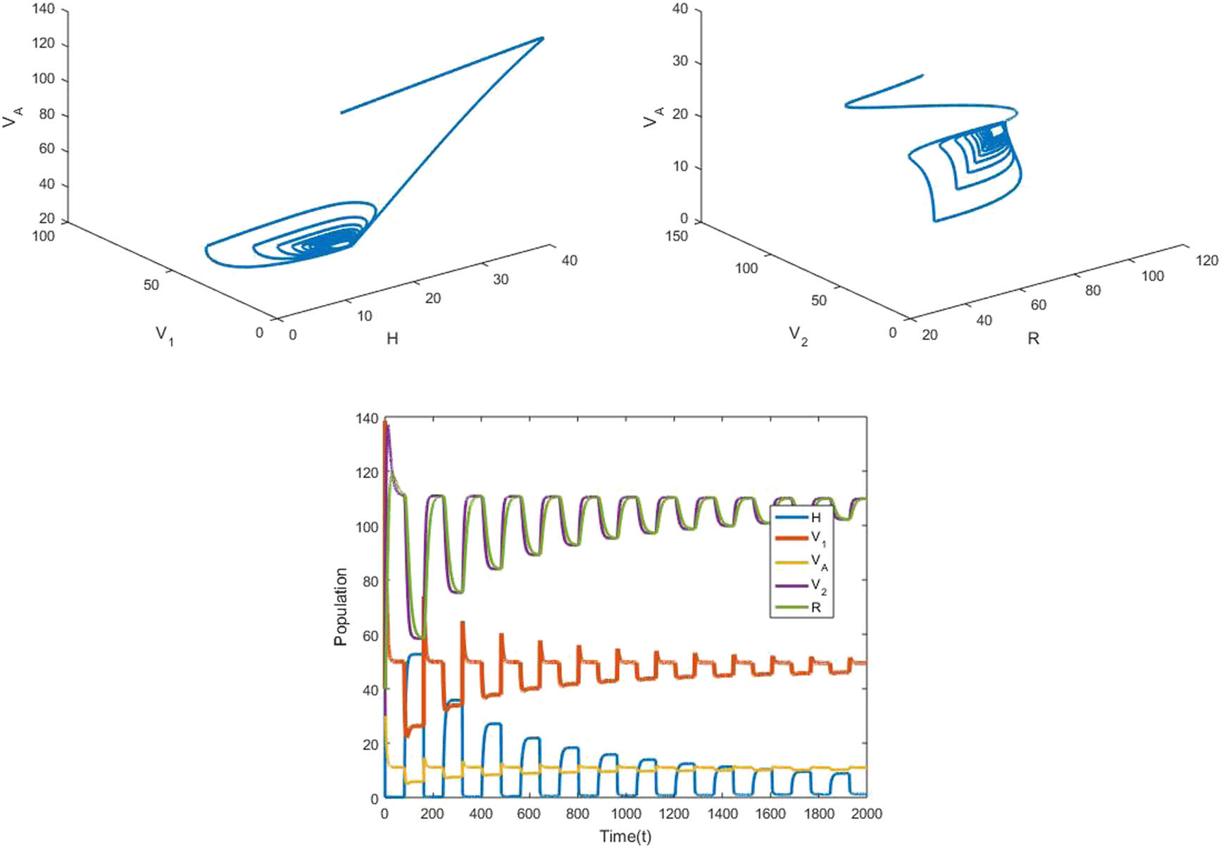
Dynamics of the system at

Dynamics of the system at

Stable dynamics of the system at
5.2 Numerical illustration for developed queuing model
In this section, we have numerically verified the results provided for the queuing model. The expected value of individuals in different states are studied, and hence, the respective graphs are plotted with respect to equally slotted time interval. The Runge-Kutta (RK) method in Section 5.2 of the fourth order is employed for this purpose and is implemented via MATLAB’s “ode45” function. The default values of the system parameters are the same as provided in Table 2. The remaining parameters have default values
We have studied the trend of the expected number of individuals in the vaccination dose 1 state, vaccination dose 2 state, and recovery state with respect to time. We observe in Figure 7 that as there is an increase in
![Figure 7
(a) Effect of
v
v
on
E
[
V
1
]
E\left[{V}_{1}]
. (b) Effect of
v
′
v^{\prime}
on
E
[
V
2
]
E\left[{V}_{2}]
.](/document/doi/10.1515/cmb-2022-0147/asset/graphic/j_cmb-2022-0147_fig_007.jpg)
(a) Effect of
![Figure 8
(a) Effect of
γ
\gamma
on
E
[
V
2
]
E\left[{V}_{2}]
. (b) Effect of
γ
\gamma
on
E
[
R
]
E\left[R]
.](/document/doi/10.1515/cmb-2022-0147/asset/graphic/j_cmb-2022-0147_fig_008.jpg)
(a) Effect of
6 Conclusion
To help guide decision-making, we propose here a novel model and analyze the dynamics in regard to the first and second vaccine dose delays/retrials. To prevent the collapse of the complex inoculation system, the vaccination of the general public must be done efficiently. A queuing model with five states, namely, healthy, vaccination (dose 1 and dose 2), after effects, and recovery is analyzed. We found the equilibrium point
-
Funding information: This research received no specific grant from any funding agency, commercial or non-profit section.
-
Conflict of interest: All authors declare no conflicts of interest in this paper.
-
Ethical approval: The conducted research is not related to either human or animal use.
-
Data availability statement: Data sharing is not applicable to this article as no datasets were generated or analyzed during the current study.
References
[1] Adongo, F. A., Lawrence, O. O., Bonyo, J., Lawi, G., & Elisha, O. A. (2020). A delayed vaccination model for rotavirus infection. European Journal of Pure and Applied Mathematics, 13(4), 840–851. 10.29020/nybg.ejpam.v13i4.3822Search in Google Scholar
[2] Agaba, G., Kyrychko, Y., & Blyuss, K. (2017). Dynamics of vaccination in a time-delayed epidemic model with awareness. Mathematical Biosciences, 294, 92–99. 10.1016/j.mbs.2017.09.007Search in Google Scholar PubMed
[3] Akman, O., Chauhan, S., Ghosh, A., Liesman, S., Michael, E., Mubayi, A., … , & Tripathi, J. P. (2022). The hard lessons and shifting modeling trends of covid-19 dynamics: Multiresolution modeling approach. Bulletin of Mathematical Biology, 84(1), 1–30. 10.1007/s11538-021-00959-4Search in Google Scholar PubMed PubMed Central
[4] Alenany, E., & El-Bas, M. A. (2017). Modelling a hospital as a queueing network: analysis for improving queueing performance. International Journal of Industrial and Manufacturing Engineering, 11, 1181–1187. Search in Google Scholar
[5] Amaku, M., Covas, D. T., Coutinho, F. A. B., Azevedo, R. S., & Massad, E. (2021). Modelling the impact of delaying vaccination against sars-cov-2 assuming unlimited vaccine supply. Theoretical Biology and Medical Modelling, 18(1), 1–11. 10.1186/s12976-021-00143-0Search in Google Scholar PubMed PubMed Central
[6] Bhagat, A. (2020). Unreliable priority retrial queues with double orbits and discouraged customers. Advancements in Mathematics and its Emerging Areas, 2214. 10.1063/5.0003372Search in Google Scholar
[7] Caga-Anan, R. L., Raza, M. N., Labrador, G. S. G., Metillo, E. B., delCastillo, P., & Mammeri, Y. (2021). Effect of vaccination to covid-19 disease progression and herd immunity. Computational and Mathematical Biophysics, 9(1), 262–272. 10.1515/cmb-2020-0127Search in Google Scholar
[8] Curry, G. L., Moya, H., Erraguntla, M., & Banerjee, A. (2021). Transient queueing analysis for emergency hospital management. IISE Transactions on Healthcare Systems Engineering, 12(1), 36–51. 10.1080/24725579.2021.1933655Search in Google Scholar
[9] Erman, S., Sevindir, H. K., & Demir, A. (2018). The stability analysis of a system with two delays. Boundary Value Problems, 2018(1), 1–11. 10.1186/s13661-018-1024-9Search in Google Scholar
[10] Gonzalez-Parra, G. (2021). Analysis of delayed vaccination regimens: A mathematical modeling approach. Epidemiologia, 2(3), 271–293. 10.3390/epidemiologia2030021Search in Google Scholar PubMed PubMed Central
[11] Kannan, S., & Ramakrishnan, S. (2016). Performance analysis of cloud computing in healthcare system using tandem queues. International Journal of Intelligent Engineering and Systems, 10, 256–264. 10.22266/ijies2017.0831.27Search in Google Scholar
[12] Karim, F., Chauhan, S., & Dhar, J. (2020). On the comparative analysis of linear and nonlinear business cycle model: Effect on system dynamics, economy and policy making in general. Quantitative Finance and Economics, 4, 172–203. 10.3934/QFE.2020008Search in Google Scholar
[13] Kumar, R., Soodan, B. S., & Sharma, S. (2021). Modelling health care queue management system facing patientas impatience using queueing theory. Reliability Theory and Applications, 16, 161–175. Search in Google Scholar
[14] Laarabi, H., Abta, A., & Hattaf, K. (2015). Optimal control of a delayed sirs epidemic model with vaccination and treatment. Acta Biotheoretica, 63, 87–97. 10.1007/s10441-015-9244-1Search in Google Scholar PubMed
[15] Malik, G., Upadhyaya, S., & Sharma, R. (2021). Particle swarm optimization and maximum entropy results for mx∕g∕1 retrial g-queue with delayed repair. International Journal of Mathematical, Engineering and Management Sciences, 6(2), 541–563. 10.33889/IJMEMS.2021.6.2.033Search in Google Scholar
[16] Meng, X., Chen, L., & Wu, B. (2010). A delay sir epidemic model with pulse vaccination and incubation times. Nonlinear Analysis: Real World Applications, 11(1), 88–98. 10.1016/j.nonrwa.2008.10.041Search in Google Scholar
[17] Obulor, R., & Eke, B. (2016). Outpatient queueing model development for hospital appointment system. International Journal of Scientific Engineering and Applied Sciences, 2, 15–22. Search in Google Scholar
[18] Rana, P., Chaudhary, K., & Chauhan, S. (2021). Dynamical analysis and optimal control problem of impact of vaccine awareness programs on epidemic system. Communications in Mathematical Biology and Neuroscience, 2021, 1–17. Search in Google Scholar
[19] Rana, P., Chauhan, S., & Mubayi, A. (2022). Burden of cytokines storm on prognosis of sars-cov-2 infection through immune response: dynamic analysis and optimal control with immunomodulatory therapy. The European Physical Journal Special Topics, 231, 1–19. 10.1140/epjs/s11734-022-00435-7Search in Google Scholar PubMed PubMed Central
[20] Rana, P., Jha, D., & Chauhan, S. (2022). Dynamical analysis on two dose vaccines in the presence of media. Journal of Computational Analysis & Applications, 30(2), 260–280.Search in Google Scholar
[21] Shim, E. (2011). Prioritization of delayed vaccination for pandemic influenza. Mathematical Biosciences and Engineering: MBE, 8(1), 95–112. 10.3934/mbe.2011.8.95Search in Google Scholar PubMed PubMed Central
[22] Singh, R. P., & Raina, A. (2018). Markovian epidemic queueing model with exposed infection and vaccination based on treatment. World Scientific News, 106, 141–150. Search in Google Scholar
[23] Upadhyaya, S. (2020). Investigating a general service retrial queue with damaging and licensed units: an application in local area networks. OPSEARCH, 57, 716–745. 10.1007/s12597-020-00440-1Search in Google Scholar
[24] Upadhyaya, S., & Khushwaha, C. (2020). Performance prediction and anfis computing for unreliable retrial queue with delayed repair under modified vacation policy. International Journal of Mathematics in Operational Research, 17(4), 437–466. 10.1504/IJMOR.2020.110843Search in Google Scholar
[25] Zhao, T., Zhang, Z., & Upadhyay, R. (2018). Delay-induced Hopf bifurcation of an sveir computer virus model with nonlinear incidence rate. Advances in Difference Equations, 256. 10.1186/s13662-018-1698-4Search in Google Scholar
[26] Zhu, H., & Liu, X. (2020). The analysis of feedback patient flow as a retrial queueing system in chinese outpatient department. Chinese Control and Decision Conference (pp. 3549–3552). Heifei, China: IEEE. 10.1109/CCDC49329.2020.9164178Search in Google Scholar
[27] Zimmerman, S., Rutherford, A. R., van der Waall, A., Norena, M., & Dodek, P. (2021). A queueing model for ventilator capacity management during the covid-19 pandemic. medRxiv. 10.1101/2021.03.17.21253488Search in Google Scholar
© 2023 the author(s), published by De Gruyter
This work is licensed under the Creative Commons Attribution 4.0 International License.
Articles in the same Issue
- Special Issue: Infectious Disease Modeling In the Era of Post COVID-19
- A comprehensive and detailed within-host modeling study involving crucial biomarkers and optimal drug regimen for type I Lepra reaction: A deterministic approach
- Application of dynamic mode decomposition and compatible window-wise dynamic mode decomposition in deciphering COVID-19 dynamics of India
- Role of ecotourism in conserving forest biomass: A mathematical model
- Impact of cross border reverse migration in Delhi–UP region of India during COVID-19 lockdown
- Cost-effective optimal control analysis of a COVID-19 transmission model incorporating community awareness and waning immunity
- Evaluating early pandemic response through length-of-stay analysis of case logs and epidemiological modeling: A case study of Singapore in early 2020
- Special Issue: Application of differential equations to the biological systems
- An eco-epidemiological model with predator switching behavior
- A numerical method for MHD Stokes model with applications in blood flow
- Dynamics of an eco-epidemic model with Allee effect in prey and disease in predator
- Optimal lock-down intensity: A stochastic pandemic control approach of path integral
- Bifurcation analysis of HIV infection model with cell-to-cell transmission and non-cytolytic cure
- Special Issue: Differential Equations and Control Problems - Part I
- Study of nanolayer on red blood cells as drug carrier in an artery with stenosis
- Influence of incubation delays on COVID-19 transmission in diabetic and non-diabetic populations – an endemic prevalence case
- Complex dynamics of a four-species food-web model: An analysis through Beddington-DeAngelis functional response in the presence of additional food
- A study of qualitative correlations between crucial bio-markers and the optimal drug regimen of Type I lepra reaction: A deterministic approach
- Regular Articles
- Stochastic optimal and time-optimal control studies for additional food provided prey–predator systems involving Holling type III functional response
- Stability analysis of an SIR model with alert class modified saturated incidence rate and Holling functional type-II treatment
- An SEIR model with modified saturated incidence rate and Holling type II treatment function
- Dynamic analysis of delayed vaccination process along with impact of retrial queues
- A mathematical model to study the spread of COVID-19 and its control in India
- Within-host models of dengue virus transmission with immune response
- A mathematical analysis of the impact of maternally derived immunity and double-dose vaccination on the spread and control of measles
- Influence of distinct social contexts of long-term care facilities on the dynamics of spread of COVID-19 under predefine epidemiological scenarios