Effect of random variation in input parameter on cracked orthotropic plate using extended isogeometric analysis (XIGA) under thermomechanical loading

2.1 Fracture analysis

The orthotropic structure with a crack is defined within global cartesian coordinates (X, Y), aligning its elastic symmetry axes with local Cartesian axes (x1, y1). The crack tip is represented using local polar coordinates (r, θ). as illustrated in Figure 1.

Figure 1

Cracked orthotropic body experiencing traction forces. This area is enclosed by the contour r and contains arbitrary boundary conditions within the designated area A.

The body encounters various forces alongside different displacement and traction boundary conditions. Expressing orthotropic stress–strain relationship by:

The relevant compliance coefficients of body are C _ij (i, j = 1, 2, 6) in local Cartesian coordinates. The stress–strain equation is given as [49]

Further, in-plane elastostatic set of equations is given as follows:

The partial differential equation governing the fourth order for an orthotropic body, derived from compatibility and equilibrium considerations, can be stated as follows: [37,38]

Complex or purely imaginary roots of Eq. (7) and are derived as ( μ k = μ k x 1 + i μ k y 1 ) which always occur in conjugate pairs as μ 1 , μ 1 ¯ and μ 2 , μ 2 ¯ .

Complex variables and analytical functions ( z k = x 1 + μ k y 1 k ( k = 1 , 2 ) ) are employed to delineate the two-dimensional displacement and stress fields surrounding the crack tip [50] The pure mode I stress components given by,

and the corresponding displacements are given as

Pure mode II stress and displacement are:

and the displacement is given as

In this scenario, K _I denotes the mode I stress intensity factors (SIF), and K _II denotes the mode II stress intensity factors (SIF). “Re” indicates the real part of the statement, while p _k and q _k are further explained below.

2.2 XIGA formulation

To effectively address problems involving discontinuities such as cracks, integrating concepts from XFEM with IGA significantly enhances their capabilities. XFEM is adept at handling static and dynamic discontinuities within structures, while IGA demonstrates precision and efficiency in analyzing complex geometries. Merging these methodologies, known as XIGA, allows for defining the entire crack independently of the mesh. XIGA essentially represents IGA approximation enriched by the application of partition of unity (PU), which is derived from the XFEM formulation.

To model singular fields and discontinuities, XIGA improves the local isogeometric approximation by introducing extra degrees of freedom at certain points near crack locations within the basic IGA model. Enrichment functions are used to contribute to overall approximation. In the XIGA method, crack-tip enrichment functions are utilized for capturing singularity within the stress fields at the crack tip, whereas Heaviside functions are employed for the representation of the crack face (Figure 2).

Figure 2

Sketch depicting the arrangement of various methods.

The generalized expression for the displacement approximation at the designated control point corresponding to ξ i is:

where u _i signifies parameters related to the particular control point; n _en refers to the number of basis functions for each element; R i p denotes the rational B-spline basis functions; n _cf denotes the number of basis functions entirely intersected by the crack face; n _ct represents the number of basis functions partially intersected by the crack tip; n _h is the count of basis functions partially intersected by the hole; and n _in indicates the number of basis functions partially intersected by the inclusion.

Additional control points influence enriched degrees of freedom as follows:

1. a _j accounts for the Heaviside function H ( ξ ) ;

2. b k a influences degrees of freedom associated with asymptotic crack-tip enrichment functions β α ;

3. c j and d j contribute to control points associated with specific functions, namely χ(ξ) and ψ(ξ) respectively, characterizing material interfaces.

Blending functions like B h and B t are employed for the Heaviside function and crack-tip function, respectively. The Heaviside function H ( ξ ) equals +1 when the parametric coordinate ξ corresponds to a particular Gauss point situated above the crack face. Conversely, when ξ lies below the crack face, H ( ξ ) equals −1.

Strain is comprised of two components in a thermomechanical problem.

Here, ε t is the total strain, ε m is the mechanical strain, ε th is the thermal strain, where ε th can be written as for plane stress state,

and for plane strain state,

Thermal expansion coefficient is denoted as α i j , and Poisson’s ratio is denoted by μ i j . According to the generalized Hooke’s law, the mechanical part of strain, ε m is shown below.

The discretized form can be written as

The displacement vector u h encompasses standard as well as additional degrees of freedom.

The displacement u h represents the standard degrees of freedom, while ‘a’ and ‘bα’ (where α ranges from 1 to 4) symbolize additional degrees of freedom utilized for the crack face and fields surrounding the crack tip. The mechanical force vector f and global stiffness matrix K are both assembled from their respective element’s contributions.

Similarly, the discretize form of thermal is

where T h is the temperature vector

Thermal force vector f th and thermal stiffness matrix Q are formed using a different matrix of basis function derivatives.

2.3 Stochastic response of MMSIF for different input random variables

This article explores the stochastic behavior of MMSIFs using the XIGA approach. It employs two probabilistic methods, namely SOPT, which relies on perturbation techniques, and direct MCS, a sampling-based method. SOPT, employing Taylor series expansion, establishes connections between certain features of random parameters and their corresponding responses. But, this method’s applicability is confined because of its dependency on lower-order polynomials. The subsequent section provides a numerical formulation outlining these methods.

3.1 Edge crack with various orientations of orthotropic axis subjected to tensile loading

We apply the proposed method to analyze an edge crack in a rectangular plate. The plate has a height-to-width ratio of 2 and a crack length-to-width ratio of 0.45, as shown in Figure 3(a). The material used is graphic epoxy with properties that are described below:

Figure 3

(a) The loading and geometry for a single edge crack with various orientations of orthotropic axis in rectangular plate, (b) NURBS mesh with enriched nodes, and (c) integral domain to calculate SIF.

E ₁ = 114.8 GPa, E ₂ = 11.7 GPa, G ₁₂ = 9.66 GPa and µ ₁₂ = 0.21.

The mesh features a uniform distribution of nodes in extended isogeometric analysis. NURBS basis functions employed are (p = q = 3) cubic, as depicted in Figure 3(b), with enriched nodes shown in Figure 3(c). The integral domain for calculating SIF is illustrated. Our results are compared with Aliabadi and Mohammadi. Figure 4 presents the SIF values for various α angles, obtained using the proposed XIGA method, Aliabadi’s FEM, and Mohammadi’s XFEM analyses.

Figure 4

Results of normalized SIFs for K _I and K _II of a single edge crack in a rectangular plate with various orientations of the orthotropic axes, at angles of α = 0° 30° 45° 60° 90° and ( K I ¯ = K I / σ πa and K II ¯ = K II / σ π a ) .

The maximum difference in mode I SIF is observed at α = 0° where a 4.3% error is observed, and for mode II, this occurs when α = 20° where a 3.6% error is observed. The results obtained by this method demonstrate that for both modes, there is an increase in normalized SIF value from α = 0° to α = 45° and then are decreased from α = 45° to α = 90°.

The effect of crack length on K _I and K _II was investigated for α = 0° orientation which is shown in Table 1 below which shows an exponential increment in K _I with an increase in crack length, and minor variation was found in K _II values.

Further study was carried out for different loading on the top edge of the plate (Tensile, Shear, Combined, and Triangular), and values of Normalized SIF, K _I, and K _II were recorded for different orientation angles (α = 0° to α = 90°), which are presented in Table 2.

The crack length taken into consideration was a/w = 0.45 and h/w = 2 as depicted in Figure 3(a), and values of K _I opening mode are more in combined loading as compared with only shear loading which is more than only tensile loading for all orientation angles. K _II shearing mode was very low in tensile loading but in shear and combined loading it was comparatively higher for all the orientation angles. For a triangular tensile load, it was obvious that the values of K _I and K _II would give lower values as the total load was half that of the uniformly distributed load.

Results of normalized K _I and K _II for different orientation angles under tensile, shear, and combined loading are depicted in Figures 5–7.

Figure 5

Normalized K _I & K _II for different orientation angles under tensile loading.

Figure 6

Normalized K _I & K _II for different orientation angles under shear loading.

Figure 7

Normalized K _I & K _II for different orientation angles for combined tensile and shear loading.

3.2 Isotropic plate with center crack under thermomechanical loading

Here, we investigate a square plate with a center crack through numerical simulations under thermomechanical loading, employing the XIGA approach. The dimensions considered are 2,000 mm × 2,000 mm, and the domain is discretized using a 50 × 50 control net. We use a NURBS basis function order of three for the simulations.

The plate contains a preexisting center crack with a length of 600 mm, as shown in Figure 8. The material properties considered are as follows:

• elastic modulus (E) = 200 GPa;

• Poisson ratio ( ν ) = 0.3;

• thermal expansion coefficient ( α ) = 11.7 × 10 − 6 C − 1 .

Figure 8

Center cracked square plate under thermomechanical loading.

The scenario involves a square plate under tensile load of 30 MPa applied at the top edge which is perpendicular to the crack. Additionally, temperature boundary conditions are applied: 0°C at the crack face and 10°C at the top edge of the plate. The bottom edge of the plate is constrained, as depicted in Figure 8.

For each step of crack extension, a crack increment of 100 mm is applied, extending proportionally from both the left and right tips. The stress intensity factors are then calculated using the domain-based interaction integral approach.

Figure 9 illustrates the stresses in x-direction (u _x ) for a/w = 0.4 subjected to thermomechanical loads, while Figure 10 shows stresses in the y-direction. Additionally, Figures 11 and 12 display the displacements along the x direction and y direction. The variation of SIFs (K _I and K _II) with the extension of the right crack tip is shown in Figure 13. The graph indicates that K _I is higher than K _II. Consequently, under combined loading conditions, the center crack in the plate exhibits opening mode behavior.

Figure 9

Stresses along x-axis.

Figure 10

Stresses along y-axis.

Figure 11

Displacement along x-axis.

Figure 12

Displacement along y-axis.

Figure 13

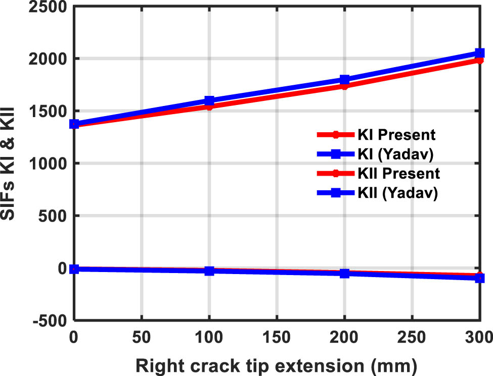
SIFs (K _I and K _II) variation of the plate subjected to thermomechanical loads is presented (validation study).

3.3 Orthotropic plate with center crack under mechanical, thermal, and thermomechanical uniaxial loading

We further analyze a center crack in a square plate under thermomechanical loads, using the XIGA approach for an orthotropic material. The square plate has initial dimensions of 2,000 mm × 2,000 mm, and the domain is discretized using a control net of size 50 × 50.

The square plate contains a preexisting center crack with a length of 600 mm, as depicted in Figure 14. This crack is analyzed when subjected to thermomechanical loading conditions using the XIGA method. The material properties considered for the analysis are as follows:

• elastic modulus (E11) = 114.8 GPa;

• elastic modulus (E22) = 11.7 GPa;

• shear modulus (G12) = 9.66 GPa;

• Poisson ratio ( ν 12 ) = 0.21;

• thermal expansion coefficient ( α 11 ) = 11.7 × 10 − 6 C − 1 ;

• thermal expansion coefficient ( α 22 ) = 2 × 10 − 5 C − 1 .

Figure 14

Center-cracked orthotropic square plate under thermomechanical loading.

Boundary conditions are as follows:

• temperature difference = 100°C;

• tensile stress on top edge = 30 MPa.

Table 3 presents the normalized SIF, K _I and K _II, for different crack lengths. The results show that K _I is consistently higher than K _II. This indicates that the center crack in the square plate primarily experiences opening mode under combined loading conditions, even for orthotropic materials. Furthermore, the analysis suggests that thermomechanical loading is more critical than pure mechanical or pure thermal loading. This is supported by the observation that as the crack length increases, the SIF values increase for all loading types.

References

[1] Viola E, Piva A, Radi E. Crack propagation in an orthotropic medium under general loading. Eng Fract Mech. 1989;34(5–6):1155–74. 10.1016/0013-7944(89)90277-4.Search in Google Scholar
[2] Nobile L, Carloni C. Fracture analysis for orthotropic cracked plates. Compos Struct. 2005;68(3):285–93. 10.1016/j.compstruct.2004.03.020.Search in Google Scholar
[3] Lim WK, Choi SY, Sankar BV. Biaxial load effects on crack extension in anisotropic solids. Eng Fract Mech. 2001;68(4):403–16. 10.1016/S0013-7944(00)00103-X.Search in Google Scholar
[4] Melenk JM, Babuška I. The partition of unity finite element method: Basic theory and applications. Comput Methods Appl Mech Eng. 1996;139(1–4):289–314. 10.1016/S0045-7825(96)01087-0.Search in Google Scholar
[5] Sukumar N, Chopp DL, Moran B. Extended finite element method and fast marching method for three-dimensional fatigue crack propagation. Eng Fract Mech. 2003;70(1):29–48. 10.1016/S0013-7944(02)00032-2.Search in Google Scholar
[6] Sukumar N, Chopp DL, Moes N, Belytschko T. Modeling holes and inclusions by level sets in the extended finite-element method. Comput Methods Appl Mech Eng. 2001;190(46–47):6183–200.10.1016/S0045-7825(01)00215-8Search in Google Scholar
[7] Asadpoure A, Mohammadi S, Vafai A. Modeling crack in orthotropic media using a coupled finite element and partition of unity methods. Finite Elem Anal Des. 2006;42(13):1165–75. 10.1016/j.finel.2006.05.001.Search in Google Scholar
[8] Asadpoure A, Mohammadi S, Vafai A. Crack analysis in orthotropic media using the extended finite element method. Thin-Walled Struct. 2006;44(9):1031–8. 10.1016/j.tws.2006.07.007.Search in Google Scholar
[9] Motamedi D, Mohammadi S. Dynamic crack propagation analysis of orthotropic media by the extended finite element method. Int J Fract. 2010;161(1):21–39. 10.1007/s10704-009-9423-7.Search in Google Scholar
[10] Motamedi D, Mohammadi S. Dynamic analysis of fixed cracks in composites by the extended finite element method. Eng Fract Mech. 2010;77(17):3373–93. 10.1016/j.engfracmech.2010.08.011.Search in Google Scholar
[11] Esna Ashari S, Mohammadi S. Fracture analysis of FRP-reinforced beams by orthotropic XFEM. J Compos Mater. 2012;46(11):1367–89. 10.1177/0021998311418702.Search in Google Scholar
[12] Hughes TJR, Cottrell JA, Bazilevs Y. Isogeometric analysis: CAD, finite elements, NURBS, exact geometry and mesh refinement. Comput Methods Appl Mech Eng. 2005;194(39–41):4135–95. 10.1016/j.cma.2004.10.008.Search in Google Scholar
[13] Manh ND, Evgrafov A, Gersborg AR, Gravesen J. Isogeometric shape optimization of vibrating membranes. Comput Methods Appl Mech Eng. 2011;200(13–16):1343–53. 10.1016/j.cma.2010.12.015.Search in Google Scholar
[14] Qian X, Sigmund O. Isogeometric shape optimization of photonic crystals via Coons patches. Comput Methods Appl Mech Eng. 2011;200(25–28):2237–55. 10.1016/j.cma.2011.03.007.Search in Google Scholar
[15] Casanova CF, Gallego A. NURBS-based analysis of higher-order composite shells. Compos Struct. 2013;104:125–33. 10.1016/j.compstruct.2013.04.024.Search in Google Scholar
[16] Benson DJ, Bazilevs Y, Hsu MC, Hughes TJ. A large deformation, rotation-free, isogeometric shell. Comput Methods Appl Mech Eng. 2011;200(13–16):1367–78. 10.1016/j.cma.2010.12.003.Search in Google Scholar
[17] Valizadeh N, Natarajan S, Gonzalez-Estrada OA, Rabczuk T, Bui TQ, Bordas SPA. NURBS-based finite element analysis of functionally graded plates: Static bending, vibration, buckling and flutter. Compos Struct. 2013;99:309–26. 10.1016/j.compstruct.2012.11.008.Search in Google Scholar
[18] Thai CH, Ferreira AJM, Carrera E, Nguyen-Xuan H. Isogeometric analysis of laminated composite and sandwich plates using a layerwise deformation theory. Compos Struct. 2013;104:196–214. 10.1016/j.compstruct.2013.04.002.Search in Google Scholar
[19] Mohammadi S, Ghorashi SS, Valizadeh N. Extended isogeometric analysis for simulation of stationary and propagating cracks. Int J Numer Methods Eng. 2011;89:1069–101.10.1002/nme.3277Search in Google Scholar
[20] De Luycker E, Benson DJ, Belytschko T, Bazilevs Y, Hsu MC. X-FEM in isogeometric analysis for linear fracture mechanics. Int J Numer Methods Eng. 2011;87(6):541–65.10.1002/nme.3121Search in Google Scholar
[21] Yao XF, Xu W, Arakawa K, Takahashi K, Mada T. Dynamic optical visualization on the interaction between propagating crack and stationary crack. Opt Lasers Eng. 2005;43(2):195–207. 10.1016/j.optlaseng.2004.06.003.Search in Google Scholar
[22] Tabarraei A, Sukumar N. Extended finite element method on polygonal and quadtree meshes. Comput Methods Appl Mech Eng. 2008;197(5):425–38. 10.1016/j.cma.2007.08.013.Search in Google Scholar
[23] Bayesteh H, Afshar A, Mohammdi S. Thermo-mechanical fracture study of inhomogeneous cracked solids by the extended isogeometric analysis method. Eur J Mech A/Solids. 2015;51:123–39. 10.1016/j.euromechsol.2014.12.004.Search in Google Scholar
[24] Yadav A, Patil RU, Singh SK, Godara RK, Bhardwaj G. A thermo-mechanical fracture analysis of linear elastic materials using XIGA. Mech Adv Mater Struct. 2022;29(12):1730–55. 10.1080/15376494.2020.1838006.Search in Google Scholar
[25] Lal A, Vaghela MB, Mishra K. Numerical analysis of an edge crack isotropic plate with void/inclusions under different loading by implementing XFEM. J Appl Comput Mech. 2021;7(3):1362–82. 10.22055/jacm.2019.31268.1848.Search in Google Scholar
[26] Lal A, Mishra K. Stochastic MMSIF of multiple edge cracks FGMs plates subjected to combined loading using XFEM. Curved Layer Struct. 2020;7(1):35–47. 10.1515/cls-2020-0004.Search in Google Scholar
[27] Palekar SP, Lal A. Stochastic fracture analysis of the laminated composite plates subjected to different types of biaxially applied stresses by implementing SXFEM. Iran J Sci Technol - Trans Mech Eng. 2022;46(2):509–30. 10.1007/s40997-021-00434-4.Search in Google Scholar
[28] Chopra PS, Wang PY, Hartz BJ. Probabilistic prediction of multiple fracture under service conditions. Nucl Eng Des. 1974;28(3):446–58. 10.1016/0029-5493(74)90213-1.Search in Google Scholar
[29] Rahman S. Probabilistic fracture mechanics: J-estimation and finite element methods. Am Soc Mech Eng Press Vessel Pip Div PVP. 1998;373:9–18.Search in Google Scholar
[30] Chen G, Rahman S, Park YH. Shape sensitivity and reliability analyses of linear-elastic cracked structures. Int J Fract. 2001;112(3):223–46. 10.1023/A:1013543913779.Search in Google Scholar
[31] Wu XF, Dzenis YA. Experimental determination of probabilistic edge-delamination strength of a graphite-fiber/epoxy composite. Compos Struct. 2005;70(1):100–8. 10.1016/j.compstruct.2004.08.016.Search in Google Scholar
[32] Alkhateb H, Al-Ostaz A, Alzebdeh KI. Developing a stochastic model to predict the strength and crack path of random composites. Compos Part B Eng. 2009;40(1):7–16. 10.1016/j.compositesb.2008.09.001.Search in Google Scholar
[33] Chowdhury MS, Song C, Gao W. Probabilistic fracture mechanics by using Monte Carlo simulation and the scaled boundary finite element method. Eng Fract Mech. 2011;78(12):2369–89. 10.1016/j.engfracmech.2011.05.008.Search in Google Scholar
[34] Rahman S, Chakraborty A. Stochastic multiscale fracture analysis of three-dimensional functionally graded composites. Eng Fract Mech. 2011;78(1):27–46. 10.1016/j.engfracmech.2010.09.006.Search in Google Scholar
[35] Sobey AJ, Blake JIR, Shenoi RA. Monte Carlo reliability analysis of tophat stiffened composite plate structures under out of plane loading. Reliab Eng Syst Saf. 2013;110:41–9. 10.1016/j.ress.2012.08.011.Search in Google Scholar
[36] Vu-Bac N, Rafiee R, Zhuang X, Lahmer T, Rabczuk T. Uncertainty quantification for multiscale modeling of polymer nanocomposites with correlated parameters. Compos Part B Eng. 2015;68:446–64. 10.1016/j.compositesb.2014.09.008.Search in Google Scholar
[37] Lal A, Mulani SB, Kapania RK. Stochastic critical stress intensity factor response of single edge notched laminated composite plate using displacement correlation method. Mech Adv Mater Struct. 2020;27(14):1223–37. 10.1080/15376494.2018.1506067.Search in Google Scholar
[38] Lal A, Palekar SP. Stochastic fracture analysis of laminated composite plate with arbitrary cracks using X-FEM. Int J Mech Mater Des. 2017;13(2):195–228. 10.1007/s10999-015-9325-y.Search in Google Scholar
[39] Hosseini SS, Bayesteh H, Mohammadi S. Thermo-mechanical XFEM crack propagation analysis of functionally graded materials. Mater Sci Eng A. 2013;561:285–302. 10.1016/j.msea.2012.10.043.Search in Google Scholar
[40] Bayesteh H, Mohammadi S. XFEM fracture analysis of orthotropic functionally graded materials. Compos Part B Eng. 2013;44(1):8–25. 10.1016/j.compositesb.2012.07.055.Search in Google Scholar
[41] Prasad NNV, Aliabadi MH, Rooke DP. The dual boundary element method for thermoelastic crack problems. Int J Fract. 1994;66(3):255–72. 10.1007/BF00042588.Search in Google Scholar
[42] Raveendra ST, Banerjee PK. Boundary element analysis of cracks in thermally stressed planar structures. Int J Solids Struct. 1992;29(18):2301–17. 10.1016/0020-7683(92)90217-H.Search in Google Scholar
[43] Shih CF, Moran B, Nakamura T. Energy release rate along a three-dimensional crack front in a thermally stressed body. Int J Fract. 1986;30(2):79–102. 10.1007/BF00034019.Search in Google Scholar
[44] Wilson WK, Yu IW. The use of the J-integral in thermal stress crack problems. Int J Fract. 1979;15(4):377–87. 10.1007/BF00033062.Search in Google Scholar
[45] Dimitri R, De Lorenzis L, Wriggers P, Zavarise G. NURBS- and T-spline-based isogeometric cohesive zone modeling of interface debonding. Comput Mech. 2014;54:369–88. 10.1007/s00466-014-0991-7.Search in Google Scholar
[46] Dimitri R, Fantuzzi N, Tornabene F, Zavarise G. Innovative numerical methods based on SFEM and IGA for computing stress concentrations in isotropic plates with discontinuities. Int J Mech Sci. 2016;118:166–87. 10.1016/j.ijmecsci.2016.09.020.Search in Google Scholar
[47] Dimitri R, Fantuzzi N, Li Y, Tornabene F. Numerical computation of the crack development and SIF in composite materials with Xfem and Sfem. Compos Struct. 2016;160:468–90. 10.1016/j.compstruct.2016.10.067.Search in Google Scholar
[48] Dimitri R, Rinaldi M, Trullo M. Theoretical and computational investigation of the fracturing behavior of anisotropic geomaterials. Contin Mech Thermodyn. 2023;35(4):1417–32. 10.1007/s00161-022-01141-4.Search in Google Scholar
[49] Asadpoure A, Mohammadi S. Developing new enrichment functions for crack simulation in orthotropic media by the extended finite element method. Int J Numer Methods Eng. 2007;69:2150–72.10.1002/nme.1839Search in Google Scholar
[50] Sih GRI, Co G, Paris PC. On cracks in rectiltnearly anisotropic bodies. Int J Fract. 1965;1:189–203.10.1007/BF00186854Search in Google Scholar
[51] Haldar SMA. Book review. Nippon Genshiryoku Gakkaishi/J Energy Soc Jpn. 2001;43(7):675.Search in Google Scholar
[52] Akramin MRM, Alshoaibi A, Hadi MSA, Ariffin AK, Mohamed NAN. Probabilistic analysis of linear elastic cracked structures. J Zhejiang Univ Sci A. 2007;8(11):1795–9. 10.1631/jzus.2007.A1795.Search in Google Scholar
© 2024 the author(s), published by De Gruyter
This work is licensed under the Creative Commons Attribution 4.0 International License.
Articles in the same Issue
- Research Articles
- Flutter investigation and deep learning prediction of FG composite wing reinforced with carbon nanotube
- Experimental and numerical investigation of nanomaterial-based structural composite
- Optimisation of material composition in functionally graded plates for thermal stress relaxation using statistical design support system
- Tensile assessment of woven CFRP using finite element method: A benchmarking and preliminary study for thin-walled structure application
- Reliability and sensitivity assessment of laminated composite plates with high-dimensional uncertainty variables using active learning-based ensemble metamodels
- Performances of the sandwich panel structures under fire accident due to hydrogen leaks: Consideration of structural design and environment factor using FE analysis
- Recycling harmful plastic waste to produce a fiber equivalent to carbon fiber reinforced polymer for reinforcement and rehabilitation of structural members
- Effect of seed husk waste powder on the PLA medical thread properties fabricated via 3D printer
- Finite element analysis of the thermal and thermo-mechanical coupling problems in the dry friction clutches using functionally graded material
- Strength assessment of fiberglass layer configurations in FRP ship materials from yard practices using a statistical approach
- An enhanced analytical and numerical thermal model of frictional clutch system using functionally graded materials
- Using collocation with radial basis functions in a pseudospectral framework to the analysis of laminated plates by the Reissner’s mixed variational theorem
- A new finite element formulation for the lateral torsional buckling analyses of orthotropic FRP-externally bonded steel beams