Three-dimensional distribution of nutrients and phytoplankton biomass in a semi-enclosed region of the Gulf of California during different ENSO phases

2.1 Study area

The Bay of La Paz is the largest and deepest coastal environment within the Gulf of California (Figure 1). It is located approximately 200 km from where the Gulf meets the Pacific Ocean, in the southeastern Baja California peninsula. This area is well-known for its high biological diversity and serves as a refuge and feeding habitat for numerous species, including some that are threatened or endangered (Durán-Campos et al. 2020).

Figure 1:

Location of (a) the Gulf of California, and (b) the Bay of La Paz. ᛫ Symbols represent the localities sampled in this study. Bathymetry is shown in m.

The bay connects directly to the Gulf of California through two openings: the San Lorenzo Channel to the southeast and Boca Grande to the northeast. The San Lorenzo Channel is narrow (20 m deep) and shallow (6 km wide). In contrast, Boca Grande is deep (250 m deep) and wide (32 km). Boca Grande is the primary area for the transport and exchange of water masses between the bay and the Gulf of California.

The bathymetry of the bay is complex, featuring a series of bathymetric sills in its northern portion where it connects with the Gulf. The maximum depth of the bay is 420 m, found in the central region known as Cuenca Alfonso. In the southern area, the depth decreases to 20 m and is characterized by slopes and extensive beaches (Molina-Cruz et al. 2002).

The regional climate is classified as desertic (type BwH), characterized by evaporation rates that exceed precipitation (García 1989). Notably, there is no river discharge into the bay. A significant feature of the region is the wind pattern, which experiences considerable seasonal variations. During winter (December to March), strong and persistent dry winds from the northwest, exceeding 12 m s⁻¹, dominate the area. In contrast, during summer (June to September), the wind pattern reverses, bringing weaker and wetter winds from the southeast, with speeds less than 5 m s⁻¹, and frequent calm periods (Monreal-Gomez et al. 2001).

The depth of the thermocline and nutricline, along with the mixing of the water column, is directly linked to these wind patterns. The wind promotes a cyclonic eddy in the bay, which plays a crucial role in supplying nutrients to the euphotic layer, essential for phytoplankton communities.

The thermohaline structure of the bay consists of four main water masses: Tropical Surface Water (TSW, S < 34.90, and T ≥ 18.00 °C), Gulf of California Water (GCW, S > 34.90, and T ≥ 12.00 °C), Subtropical Subsurface Water (StSsW, 34.50 < S < 34.90, and 9.00 ≤ T ≤ 18.00 °C), and Pacific Intermediate Water (PIW, 34.50 ≤ S < 34.80, and 4.00 ≤ T < 9.00 °C). The PIW is specifically found in the Boca Grande region, off the bay (Coria-Monter et al. 2019b; Monreal-Gómez et al. 2001).

Within the bay, both surface and subsurface circulation are dominated by a cyclonic eddy, which significantly affects the distribution of phytoplankton organisms. This cyclonic eddy leads Ekman pumping, which fertilizes the euphotic layer (Coria-Monter et al. 2017) and causes phytoplankton to aggregate differentially from the center towards the periphery (Coria-Monter et al. 2014). Furthermore, additional processes like the propagation of internal waves and hydraulic jumps increase the variability of the water column, thereby enhancing phytoplankton biomass (Coria-Monter et al. 2019c).

2.2 Sampling

The data set used in this study was collected during two oceanographic cruises. The first, known as the Paleaomar-1 cruise, took place in November 2014, while the second cruise, Paleomar-2, was conducted in November 2016. Both cruises were carried out onboard the R/V El Puma, operated by the National Autonomous University of Mexico. The sampling strategy involved an equidistant grid consisting of 44 hydrographic stations that covered the interior of the bay and its connection to the Gulf of California (Figure 1).

At each station, hydrographic data were collected using a CTD probe (SeaBird 19 plus), which has a precision of 0.005 °C for temperature, and 0.0005 S m⁻¹ for conductivity. The CTD was attached to a Rosette System containing 12 Niskin bottles (General Oceanics) with a capacity of 10 l each. The CTD-Rosette system was deployed from the water surface to 5 m above the seafloor, descending at a speed of 1 m s⁻¹, with data being acquired at a frequency of 24 Hz.

Water samples for nutrients and Chl-a analyses were collected at different depths: surface, 10, 30, and 50 m depth. Once the Rosette System was onboard, 100-ml subsamples for nutrient determinations were filtered through two cellulose acetate syringe filters (Merck Millipore, 0.22-μm and 0.45-μm pore sizes). These subsamples were then stored in polypropylene containers that had been previously washed with an acid solution, fixed with chloroform, and kept frozen at −20 °C until laboratory analysis.

For Chl-a determinations, 4-l subsamples were filtered through nitrocellulose membrane filters (Merck Millipore, 0.45-μm pore size) using a stainless-steel vacuum manifold system set at 10 psi. During the filtration process, special precautions were taken to avoid contamination, including rinsing the manifold system with distilled water between each sample and conducting the procedure under low-light conditions to prevent degradation. Finally, the membranes were stored in plastic centrifuge tubes covered with aluminum foil and frozen at −20 °C prior to analysis.

2.3 Laboratory chemical analyses

The water samples collected for nutrient analysis were analyzed in the laboratory immediately after the research cruises. The concentrations of nitrate (precision of 0.10 µM), nitrite (precision of 0.02 µM), soluble reactive phosphorus (SRP, precision of 0.04 µM), and soluble reactive silica (SRSi, precision of 0.10 µM) were determined using a segmented flow analyzer (Skalar San Plus) following the methods outlined by Grasshoff et al. (1983) and Kirkwood (1994).

For the quantification of Chl-a, 90 % acetone was added to the centrifuge tubes containing the membranes. The samples were extracted in the dark for 24 h and then stored at −20 °C. After this extraction period, the tubes were centrifuged at 2,490g (Eppendorf 5,840 centrifuge) for 30 min. Finally, in accordance with the methodology of Strickland and Parsons (1972), the absorbance was measured in triplicate at wavelengths of 750, 664, 647, and 630 nm using a spectrophotometer (Genesys 10S UV-VIS, Thermo Scientific) with quartz cells. This entire process was carried out under extremely low lighting conditions.

2.4 Data analyses

To identify the ENSO phases that occurred during each research cruise, the Ocean Niño Index (ONI) provided by the NOAA National Weather Service was used (https://origin.cpc.ncep.noaa.gov/products/analysis_monitoring/ensostuff/ONI_v5.php). The ONI is a reliable indicator for monitoring the evolution and strength of ENSO events in the El Niño 3.4 oceanic region. According to this index, values higher than +0.5 indicate El Niño conditions, while values lower than −0.5 indicate La Niña conditions.

The CTD data were initially processed with the nominal calibration file, following the routines and subroutines of the manufacturer with SBE Data Processing software V.7.26.7, averaging each dbar. Then, salinity and temperature were derived using standard algorithms. To analyze the presence and proportions of the water masses in both research cruises, temperature-salinity (TS) diagrams were constructed based on the classification outlined by Lavín et al. (2009).

Wind data for November 2014 and November 2016 were obtained from meteorological station # 76404, operated by the National Meteorological Service of Mexico (Servicio Meteorológico Nacional) and located in La Paz city. This dataset included records of wind magnitude and direction recorded every 15 min. To eliminate high-frequency fluctuations, a 24-h running average was applied.

3.1 ENSO phases

During the Paleomar-1 cruise in November 2014, the ONI recorded a value of +0.6 indicating the presence of an El Niño event. In contrast, during the Paleomar-2 cruise in November 2016, a value of −0.7 was registered, signifying La Niña conditions. Thus, both events exhibited similar intensity.

3.2 Hydrography

The T-S diagrams generated indicated notable differences in the number and proportion of water masses observed during the two research cruises (Figure 2).

Figure 2:

Temperature-salinity diagram of both research cruises considered in this study. Red points, Paleomar-1 cruise, November 2014; blue points, Paleomar-2 cruise, November 2016; StSsW, subtropical subsurface water; GCW, Gulf of California water; TSW, tropical surface water; PIW, Pacific intermediate water.

During the Paleomar-1 cruise, four distinct water masses were identified: (1) Subtropical Subsurface Water, (2) Gulf of California Water, (3) Tropical Surface Water, and (4) Pacific Intermediate Water (Figure 2). The PIW was limited to stations in the region connecting the bay to the Gulf of California.

In contrast, only three water masses were identified during Paleomar-2 cruise, as there was no evidence of TSW. The observed water masses were (1) GCW, (2) StSsW, and (3) PIW, which was also confined to the stations linked to the Gulf.

The horizontal and vertical temperature distributions demonstrated distinct patterns during the two cruises analyzed in this study.

During the Paleomar 1 cruise, it was noted that the temperature at surface (Figure 3a), at 10 m (Figure 3b), and at 30 m depth (Figure 3c) remained largely uniform across the bay, at around 26.50 °C, except for the Boca Grande region, where temperatures dropped to approximately 25.50 °C. In contrast, at a depth of 50 m (Figure 3d), temperature gradients were observed, with colder cores (22–23 °C) located in the northern and southwestern parts of the bay.

Figure 3:

Horizontal distribution of temperature (°C) at different depths: (a) surface, (b) 10, (c) 30, and (d) 50 m depth during the Paleomar-1 cruise, (e) surface, (f) 10, (g) 30, and (h) 50 m depth during the Paleomar-2 cruise.

During the Paleomar 2 cruise, temperature distribution showed higher temperatures compared to the Paleomar 1 cruise. In the first three depth levels (surface, 10 and 30 m depth), temperatures exceeded 27.50 °C and were uniformly distributed throughout the bay (Figure 3e–g). However, at 30 m depth, a small area of lower temperature was observed (Figure 3g). At 50 m depth, horizontal temperature gradients began to emerge, revealing a cold core (<22.00 °C) in the Alfonso Basin. In contrast, higher temperatures (>27.00 °C) were recorded in the southern bay, where strong horizontal temperature gradients were also noted (Figure 3h).

3.3 Wind field

The wind dataset collected during each research cruise exhibited notable differences. For example, during the Paleomar-1 cruise held in November 2014, the prevailing winds were northeasterly, with speeds exceeding 4 m s⁻¹. Occasional southwesterly winds were also during the month, but these were brief (Figure 4a). In contrast, during the Paleomar-2 cruise, which took place in November 2016, the northeasterly winds were dominant, with only brief occurrences of weak southwesterly wind, typically with speeds below 1 m s⁻¹ (Figure 4b). Additionally, the wind speeds in 2016 were more consistent compared to those recorded in 2014. It is important to note that during the Paleomar-1 cruise, the northeasterly winds exceeded 4 m s⁻¹ on two lapses (Figure 4a), while during the Paleomar-2 cruise, the wind speeds, were around 3 m s⁻¹ (Figure 4b).

Figure 4:

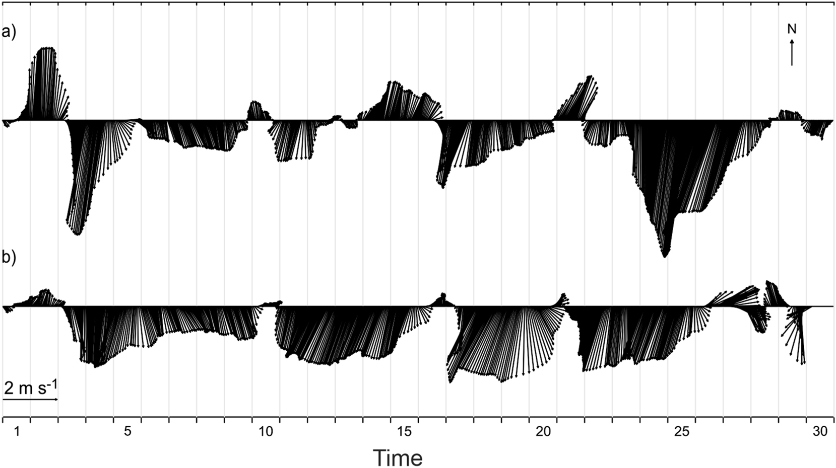
Wind velocity (m s⁻¹) time series at weather station at La Paz, Baja California Sur, during (a) November 2014 (the Paleomar-1 cruise), (b) November 2016 (the Paleomar-2 cruise).

3.4 Nutrients

The nutrient concentrations and their horizontal distribution exhibited variations with depth and between the two research cruises.

During the Paleomar-1 cruise, at the surface, nitrate concentrations ranged from 0.07 to 2.41 µM, with the highest value recorded in a core located in the southwestern region of the bay (Figure 5a). Nitrite concentrations (Figure 6a) varied from 0.04 to 0.46 µM, showing two cores: one at the boundary with the Gulf of California and another in the southwestern region near the San Lorenzo Channel. SRP values ranged from 0.24 to 0.76 µM, exhibiting lower concentrations in the central portion of the bay (Figure 7a). Additionally, SRSi varied from 0.03 to 26.20 µM, with two high-concentration cores observed in the western section of the bay (Figure 8a).

Figure 5:

Horizontal distribution of nitrate (µM) at different depths: (a–d) Paleomar-1 cruise; (e–h) Paleomar-2 cruise.

Figure 6:

Horizontal distribution of nitrites (µM) at different depths: (a–d) Paleomar-1 cruise; (e–h) Paleomar-2 cruise.

Figure 7:

Horizontal distribution of soluble reactive phosphorus (µM) at different depths: (a–d) Paleomar-1 cruise; (e–h) Paleomar-2 cruise.

Figure 8:

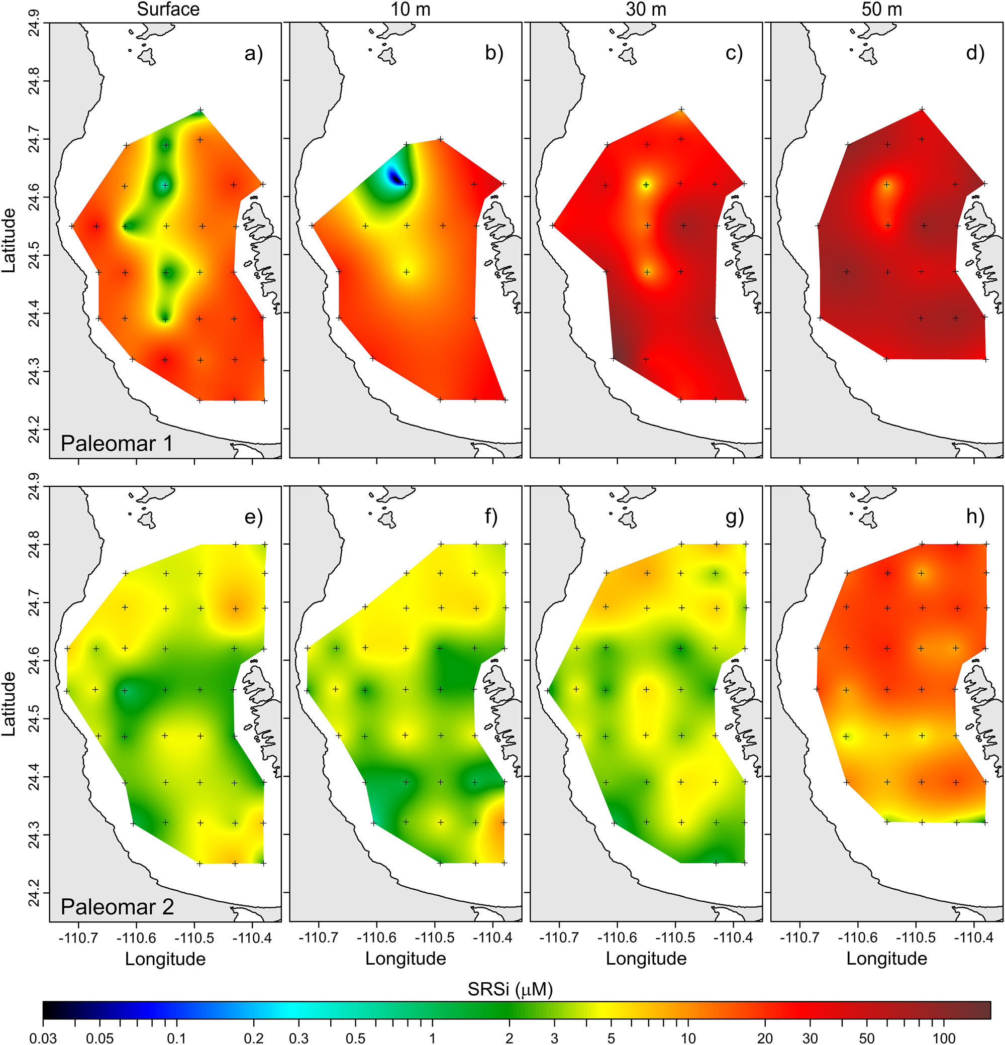
Horizontal distribution of soluble reactive Si (µM) at different depths: (a–d) Paleomar-1 cruise; (e–h) Paleomar-2 cruise.

At 10 m depth, nitrate concentrations ranged from 0.26 to 1.27 µM, with lower levels observed in the central area of the bay (Figure 5b). Nitrite concentrations varied from 0.05 to 0.64 µM, revealing two regions of high levels: one near the Gulf of California and another in the southern region near the San Lorenzo Channel (Figure 6b). SRP values ranged from 0.26 to 0.71 µM, with a core of lower concentrations also noted in the central region of the bay (Figure 7b). Finally, SRSi values ranged from 0.12 to 47.77 µM, showing high concentrations in the southwestern bay, close to the coast (Figure 8b).

At 30 m depth, nutrient concentrations were statistically higher than those observed in surface waters. Nitrate levels increased to a range of 0.56–8.79 µM, with two areas of high concentrations: one in the southwestern region near the coast and another near the San Lorenzo Channel (Figure 5c). Nitrite concentrations ranged from 0.08 to 0.57 µM, with higher values noted close to the San Lorenzo Channel (Figure 6c). SRP values ranged from 0.33 to 1.14 µM, with the highest concentrations found in the western portion of the bay, near San Juan de la Costa (Figure 7c). SRSi ranged from 1.60 to 152.46 µM, with the highest concentration observed in the San Juan de la Costa region (Figure 8c).

At 50 m depth, high concentrations of nutrients were observed. Nitrate levels ranged from 1.21 to 12.57 µM, with the highest concentrations found in the central part of the bay (Figure 5d). Nitrite levels ranged from 0.09 to 0.69 µM, displaying high values in the southern region near the San Lorenzo Channel (Figure 6d). SRP varied from 0.44 to 1.50 µM, with a peak observed in the southern area of the bay (Figure 7d). Furthermore, SRSi ranged from 5.76 to 97.62 µM, with the highest concentrations recorded in the western part of the bay (Figure 8d).

During the Paleomar-2 cruise, surface nitrate concentrations ranged from 0.00 to 0.86 µM, with lower values found in the central portion of the bay (Figure 5e). Nitrite levels varied from 0.02 to 0.37 µM, with higher concentrations observed near Boca Grande, where the bay connects to the Gulf of California (Figure 6e). SRP concentrations ranged from 0.25 to 0.55 µM, showing lower levels in the central part of the bay (Figure 7e). In contrast, SRSi concentrations varied from 0.86 to 8.97 µM, with a peak also recorded at Boca Grande, near the Gulf of California (Figure 8e).

At 10 m depth, nitrate concentrations reached up to 0.82 µM, with the highest levels found in the central portion of the bay (Figure 5f). Nitrite concentrations ranged from 0.02 to 0.32 µM, showing high levels in the central region (Figure 6f). SRP values ranged from 0.25 to 0.58 µM, revealing a core with low concentration near Roca Partida (Figure 7f). SRSi concentrations varied from 0.53 to 10.26 µM, with the highest concentrations located in the northern region of the bay (Figure 8f).

At 30 m depth, the nitrate concentration ranged from 0.02 to 2.73 µM, with the highest values found in the central and northern areas of the bay (Figure 5g). The nitrite concentration ranged from 0.02 to 0.22 µM, peaking in the central region (Figure 6g). SRP levels ranged from 0.24 to 0.67 µM, displaying a uniform distribution pattern throughout the bay (Figure 7g). The concentration of SRSi ranged from 1.10 to 8.48 µM, also showing a uniform distribution pattern (Figure 8g).

Finally, at 50 m depth, nitrate concentrations increased significantly, ranging from 0.21 to 13.22 µM, with high levels observed in the central and northern regions (Figure 5h). Nitrite concentrations varied from 0.04 to 0.50 µM, with a notable peak near the San Lorenzo Channel and a lower value in the central portion (Figure 6h). The SRP levels varied from 0.32 to 2.08 µM, showing a high concentration core in the central region of the bay (Figure 7h). Finally, SRSi concentrations ranged from 1.43 to 23.63 µM, with the highest values also located in the central region of the bay (Figure 8h).

The values of SRSi measured during the Paleomar-1 cruise were significantly higher than those recorded in the Paleomar-2 cruise, especially at 30 m depth. For example, the SRSi concentration reached 152.46 µM during the Paleomar-1 cruise (Figure 8c), whereas the highest concentration observed in the Paleomar-2 cruise was only 8.48 µM (Figure 8g).

Statistical t-tests performed on the dataset indicated significant differences, particularly at the surface, 10, and 30 m depths (Supplementary Table S1).

3.5 Chlorophyll-a

The Chl-a levels at the surface, 10, 30, and 50 m depth, within the euphotic zone exhibited variations with depth between the two cruises, which indicate changes in nutrient concentrations.

During the Paleomar-1 cruise, the surface of Chl-a concentrations ranged from 0.04 to 2.60 mg m⁻³, with the highest levels detected in a core located in the southern bay (Figure 9a). At 10 m depth, the Chl-a levels remained similar to those observed at the surface, peaking at 2.69 mg m⁻³ in the northern bay (Figure 9b). At 30 m depth, the concentrations fluctuated from 0 to 2.83 mg m⁻³, with the highest levels found in the central bay (Figure 9c). Finally, at 50 m depth, high values of up to 7.60 mg m⁻³ were recorded along the western coast of the bay (Figure 9d).

Figure 9:

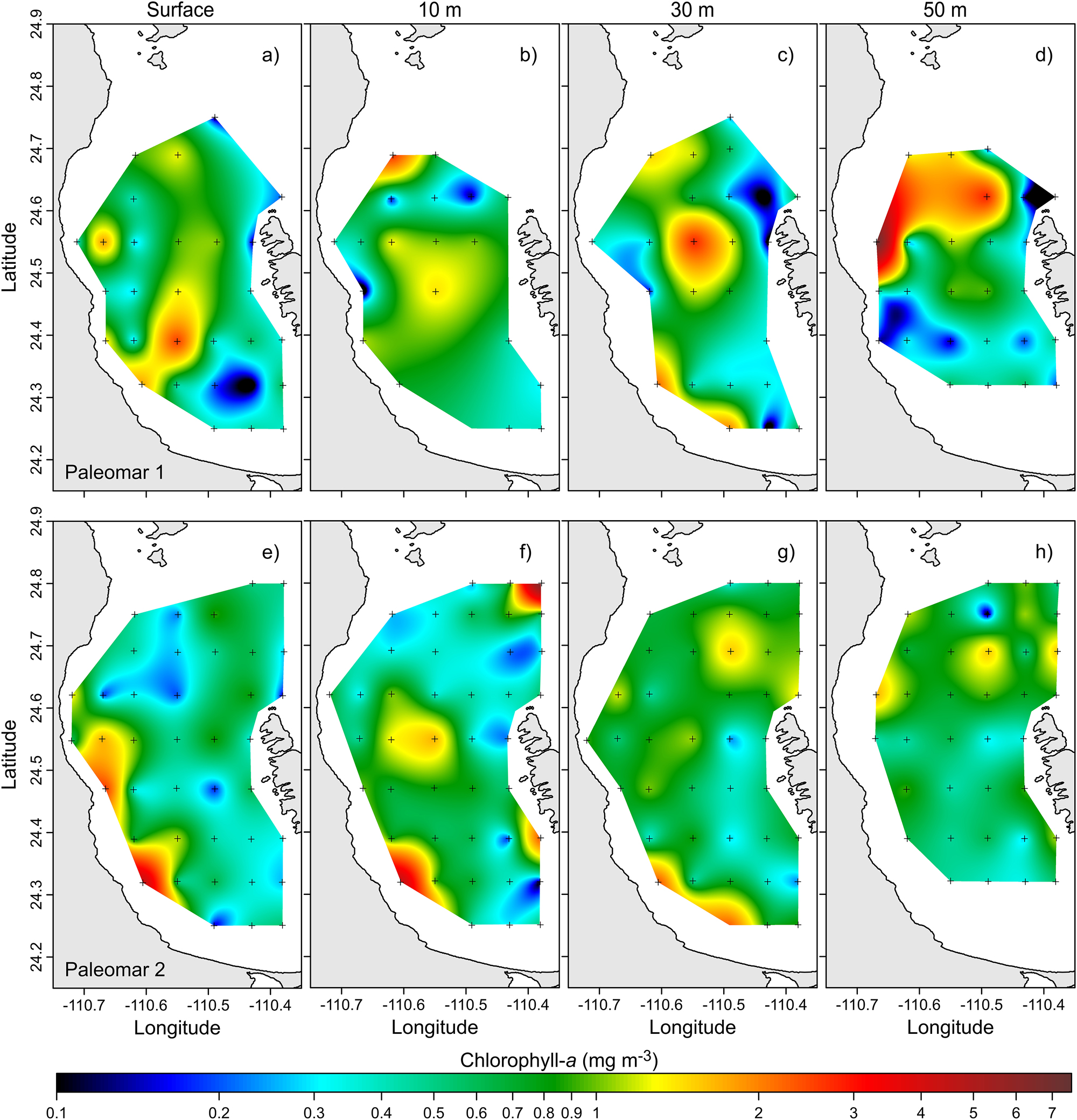
Horizontal distribution of Chl-a (mg m⁻³) levels at different depths: (a–d) Paleomar-1 cruise; (e–f) Paleomar-2 cruise.

During the Paleomar-2 cruise, the concentrations of Chl-a showed notable differences compared to those recorded in the Paleomar-1 cruise, particularly in the subsurface layers. At the surface, Chl-a values ranged from 0.13 to 4.63 mg m⁻³, with the highest concentrations found in the southern bay, specifically near San Juan de la Costa (Figure 9e). At 10 m depth, a similar distribution was observed, with peak values reaching 4.69 mg m⁻³ also in the San Juan de la Costa area (Figure 9f). At 30 m depth, Chl-a values varied from 0.21 to 2.36 mg m⁻³, again with the highest concentrations found in the southern region of the bay (Figure 9g). At 50 m depth, the maximum Chl-a value recorded was 1.70 mg m⁻³, displaying a more uniform distribution across the region (Figure 9h).

Comparing the two cruises, the concentrations of Chl-a were higher during the Paleomar-1 cruise, especially in the subsurface layers between 30 and 50 m depth.

References

Andrade, M.P., Magalhães, A., Pereira, L.C.C., Flores-Montes, M.J., Pardal, E.C., Andrade, T.P., and Costa, R.M. (2016). Effects of a La Niña event on hydrological patterns and copepod community structure in a shallow tropical estuary (Taperaçu, Northern Brazil). J. Mar. Syst. 164: 128–143.10.1016/j.jmarsys.2016.07.006Search in Google Scholar
Brierley, A.S. (2017). Plankton. Curr. Biol. 27: R478–R483, https://doi.org/10.1016/j.cub.2017.02.045.Search in Google Scholar PubMed
Coria-Monter, E., Monreal-Gómez, M.A., Salas de León, D.A., and Durán-Campos, E. (2017). Wind driven nutrient and chlorophyll-a enhancement at a cyclonic circulation in Bay of La Paz, Gulf of California, Mexico. Estuar. Coast. Shelf Sci. 196: 290–300.10.1016/j.ecss.2017.07.010Search in Google Scholar
Coria-Monter, E., Monreal-Gómez, M.A., Salas de Leon, D.A., and Durán-Campos, E. (2019b). Water masses and chlorophyll-a distribution in a semi-enclosed bay of the southern Gulf of California, Mexico, after the “Godzilla El Niño”. Arab. J. Geosci. 12: 473.10.1007/s12517-019-4636-1Search in Google Scholar
Coria-Monter, E., Monreal-Gómez, M.A., Salas-de-León, D.A., Aldeco-Ramírez, J., and Merino-Ibarra, M. (2014). Differential distribution of diatoms and dinoflagellates in a cyclonic eddy confined in the Bay of La Paz, Gulf of California. J. Geophys. Res. 119: 6258–6268, https://doi.org/10.1002/2014JC009916.Search in Google Scholar
Coria-Monter, E., Salas de León, D.A., Monreal-Gómez, M.A., and Durán-Campos. (2019a). Satellite observations of the effect of the “Godzilla El Niño” on the Tehuantepec upwelling system in the Mexican Pacific. Helgol. Mar. Res. 73: 3.10.1186/s10152-019-0525-ySearch in Google Scholar
Coria-Monter, E., Salas de Leon, D.A., Monreal-Gómez, M.A., and Durán-Campos, E. (2019c). Internal waves in the Bay of La Paz, southern Gulf of California, Mexico. Vie Milieu 69: 115–122.Search in Google Scholar
Dai, Y., Yang, S., Hu, C., Xu, W., Anderson, D.M., Li, Y., Song, X.-P., Boyce, D.G., Gibson, L., Zheng, C., et al.. (2023). Coastal phytoplankton blooms expand and intensify in the 21st century. Nature 615: 280–284, https://doi.org/10.1038/s41586-023-05760-y.Search in Google Scholar PubMed PubMed Central
Davies, C., Ajani, P., Armbrecht, L., Atkins, N., Baird, M.E., Beard, J., Bonham, P., Burford, M., Clementson, L., Coad, P., et al.. (2018). A database of chlorophyll-a in Australian waters. Sci. Data 5: 180018, https://doi.org/10.1038/sdata.2018.18.Search in Google Scholar PubMed PubMed Central
Durán-Campos, E., Monreal-Gómez, M.A., Salas de León, D.A., and Coria-Monter, E. (2020). Field and satellite observations on the seasonal variability of the surface chlorophyll-a in the Bay of La Paz, Gulf of California, Mexico. IJOO 14: 157–167, https://doi.org/10.37622/ijoo/14.1.2020.157-167.Search in Google Scholar
Falkowski, P. (2012). Ocean science: the power of plankton. Nature 483: 17–20, https://doi.org/10.1038/483s17a.Search in Google Scholar
García, E. (1989). Apuntes de climatología. Universidad Nacional Autónoma de México, Ciudad de México.Search in Google Scholar
Gaube, P., McGillicuddy, D.J., Chelton, D.B., Behrenfeld, M.J., and Strutton, P.G. (2014). Regional variations in the influence of mesoscale eddies on near-surface chlorophyll. J. Geophys. Res. 119: 8195–8220, https://doi.org/10.1002/2014jc010111.Search in Google Scholar
Grasshoff, K., Ehrhardt, M., and Kremling, K. (1983). Methods of seawater analysis, 2nd ed. Verlag Chemie, Weinheim.Search in Google Scholar
Herrera-Cervantes, H., Lluch-Cota, S., Cortés-Ramos, J., Farfan, L., and Morales-Aspeitia, R. (2020). Interannual variability of surface satellite-derived chlorophyll concentration in the bay of La Paz, Mexico, during 2003–2018 period: the ENSO signature. Cont. Shelf Res. 209: 104254.10.1016/j.csr.2020.104254Search in Google Scholar
Herrera-Cervantes, H., Lluch-Cota, S., Lluch-Cota, D., Gutiérrez de Velasco-Sanromán, G., and Lluch-Belda, D. (2010). ENSO influence on satellite-derived chlorophyll trends in the Gulf of California. Atmósfera 23: 253–262.Search in Google Scholar
Kirkwood, D.S. (1994). SanPlus segmented flow analyzer and its applications. Seawater analysis. Skalar, Amsterdam.Search in Google Scholar
Lavín, M.F., Castro, R., Beier, E., Godínez, V.M., Amador, A., and Guest, P. (2009). SST, thermohaline structure, and circulation in the southern Gulf of California in June 2004 during the North American monsoon experiment. J. Geophys. Res. Oceans 114: C02025, https://doi.org/10.1029/2008jc004896.Search in Google Scholar
Lavin, M.F. and Marinone, S.G. (2003). An overview of the physical oceanography of the Gulf of California. In: Velasco Fuentes, O.U., Sheinbaum, J., and Ochoa, J. (Eds.), Nonlinear processes in geophysical fluid dynamics. Springer Dordrecht, Netherlands, pp. 173–204.10.1007/978-94-010-0074-1_11Search in Google Scholar
Lévy, M., Franks, P.J.S., and Smith, K.S. (2018). The role of submesoscale currents in structuring marine ecosystems. Nat. Commun. 9: 4758, https://doi.org/10.1038/s41467-018-07059-3.Search in Google Scholar PubMed PubMed Central
Machado, I., Barreiro, M., and Calliari, D. (2013). Variability of chlorophyll-a in the Southwestern Atlantic from satellite images: seasonal cycle and ENSO influences. Cont. Shelf Res. 53: 102–109, https://doi.org/10.1016/j.csr.2012.11.014.Search in Google Scholar
McGillicuddyJr.D.J. (2016). Mechanisms of physical-biological-biogeochemical interaction at the oceanic mesoscale. Ann. Rev. Mar. Sci. 8: 125–159, https://doi.org/10.1146/annurev-marine-010814-015606.Search in Google Scholar PubMed
McPhaden, M.J., Santoso, S., and Cai, W. (2021). Introduction to El Niño southern oscillation in a changing climate. In: McPhaden, M.J., Santoso, A., and Cai, W. (Eds.). El Niño southern oscillation in a changing climate. American Geophysical Union, Geophysical Monograph Series, USA, pp. 1–19.10.1002/9781119548164.ch1Search in Google Scholar
Molina-Cruz, A., Pérez-Cruz, L., and Monreal-Gómez, M.A. (2002). Laminated sediments in the Bay of La Paz, Gulf of California: a depositional cycle regulated by pluvial flux. Sedimentology 49: 1401–1410, https://doi.org/10.1046/j.1365-3091.2002.00505.x.Search in Google Scholar
Monreal-Gómez, M.A., Molina-Cruz, A., and Salas de León, D.A. (2001). Water masses and cyclonic circulation in Bay of La Paz, Gulf of California, during June 1998. J. Mar. Syst. 30: 305–315, https://doi.org/10.1016/s0924-7963(01)00064-1.Search in Google Scholar
Richardson, A.J. (2008). In hot water: zooplankton and climate change. ICES J. Mar. Sci. 65: 279–295, https://doi.org/10.1093/icesjms/fsn028.Search in Google Scholar
Roesler, C., Uitz, J., Claustre, H., Boss, E., Xing, X., Organelli, E., Briggs, N., Bricaud, A., Schmechtig, C., Poteaaus, A., et al.. (2017). Recommendations for obtaining unbiased chlorophyll estimates from in situ chlorophyll fluorometers: a global analysis of WET Labs ECO sensors. L&O Methods 15: 572–585, https://doi.org/10.1002/lom3.10185.Search in Google Scholar
Roy, S., Llewellyn, C.A., Egeland, E.S., and Johnsen, G. (2011). Phytoplankton pigments: characterization, chemotaxonomy and applications in oceanography. Cambridge University Press, Cambridge.10.1017/CBO9780511732263Search in Google Scholar
Schiermeier, Q. (2015). Hunting the Godzilla El Niño. Nature 526: 490–491, https://doi.org/10.1038/526490a.Search in Google Scholar PubMed
Shafeeque, M., Balchand, A.N., Shah, P., George, G., Smitha, B.R., Varghese, E., Joseph, A.K., Sathyendranath, S., and Platt, T. (2021). Spatio-temporal variability of chlorophyll-a in response to coastal upwelling and mesoscale eddies in the south eastern Arabian Sea. Int. J. Remote Sens. 42: 4840–4867, https://doi.org/10.1080/01431161.2021.1899329.Search in Google Scholar
Sosa-Ávalos, R., Santamaría-del-Ángel, E., Acosta-Chamorro, V., Silva-Iñiguez, L., Pelayo-Martínez, G.C., and Quijano-Scheggia, S.I. (2021). Phytoplankton primary production during the cold and warm seasons in Manzanillo and Santiago Bays, Mexico. Estuar. Coast. Shelf Sci. 261: 107569, https://doi.org/10.1016/j.ecss.2021.107569.Search in Google Scholar
Strickland, J.D.H. and Parsons, T.R. (1972). A practical handbook of seawater analysis. Ottawa Fisheries Research Board of Canada, Bulletin 167, Ottawa, Canada.Search in Google Scholar
Villamaña, M., Mouriño-Carballido, B., Maranon, E., Cermeño, P., Chouciño, P., da Silva, J.C.B., Díaz, P.A., Fernández-Castro, B., Gilcoto, M., Graña, R., et al.. (2017). Role of internal waves on mixing, nutrient supply and phytoplankton community structure during spring and neap tides in the upwelling ecosystem of Ría de Vigo (NW Iberian Peninsula). Limnol. Oceanogr. 62: 1014–1030, https://doi.org/10.1002/lno.10482.Search in Google Scholar
Wijaya, A., Zakiyah, U., Sambah, A.B., and Setyohadi, D. (2020). Spatio-temporal variability of temperature and chlorophyll-a concentration of sea surface in Bali Strait, Indonesia. Biodiv 21: 5283–5290, https://doi.org/10.13057/biodiv/d211132.Search in Google Scholar
Wilkerson, F.P., Dudgale, R.C., Marchi, A., and Collins, C.A. (2002). Hydrography, nutrients and chlorophyll during El Niño and La Niña 1997–1998 winters in the Gulf of Farallones, California. Prog. Oceanogr. 54: 293–310.10.1016/S0079-6611(02)00055-1Search in Google Scholar
Xiu, P., Dai, M., Chai, F., Zhuo, K., Zeng, L., and Du, C. (2018). On contributions by wind-induced mixing and eddy pumping to interannual chlorophyll variability during different ENSO phases in the northern South China Sea. Limnol. Oceanogr. 64: 503–514, https://doi.org/10.1002/lno.11055.Search in Google Scholar
Zhang, H., Qiu, Z., Sun, D., Wang, S., and He, Y. (2017). Seasonal and interannual variability of satellite-derived chlorophyll-a (2000–2012) in the Bohai Sea, China. Remote Sens. 9: 582, https://doi.org/10.3390/rs9060582.Search in Google Scholar
Supplementary Material
This article contains supplementary material (https://doi.org/10.1515/bot-2025-0007).
© 2025 the author(s), published by De Gruyter, Berlin/Boston
This work is licensed under the Creative Commons Attribution 4.0 International License.
Articles in the same Issue
- Frontmatter
- In this issue
- Physiology and Ecology