Calibration of insulin pumps based on discrete doses at given cycle times
-
Hugo Bissig
 ,
Oliver Büker
,
Oliver Büker
 ,
Krister Stolt
,
Krister Stolt

Abstract
One application in the medical treatment at very small flow rates is the usage of an Insulin pump that delivers doses of insulin at constant cycle times for a specific basal rate as quasi-continuous insulin delivery, which is an important cornerstone in diabetes management. The calibration of these basal rates are performed by either gravimetric or optical methods, which have been developed within the European Metrology Program for Innovation and Research (EMPIR) Joint Research Project (JRP) 18HLT08 Metrology for drug delivery II (MeDDII). These measurement techniques are described in this paper, and an improved approach of the analytical procedure given in the standard IEC 60601-2-24:2012 for determining the discrete doses and the corresponding basal rates is discussed in detail. These improvements allow detailed follow up of dose cycle time and delivered doses as a function of time to identify some artefacts of the measurement method or malfunctioning of the insulin pump. Moreover, the calibration results of different basal rates and bolus deliveries for the gravimetric and the optical methods are also presented. Some analysis issues that should be addressed to prevent misinterpreting of the calibration results are discussed. One of the main issues is the average over a period of time which is an integer multiple of the cycle time to determine the basal rate with the analytical methods described in this paper.
Introduction
Very small flow rates are commonly used in several areas of pharmaceutics, health care, flow chemistry or microfluidic applications. An application in medical treatment is the use of an insulin pump that delivers small amounts of liquids at a specific time interval to deliver the insulin quasi-continuous [1], [2], [3]. The pump mechanism consist of a stepper motor that moves the plunger incrementally, which forces the piston into the container to push out the insulin. A discrete volume is often called a single dose and corresponds to the smallest delivered quantity of insulin delivered. Depending on the basal rate (insulin flow rate), the volume of the single dose and the time interval between single doses (i.e., the cycle time) are varying as we will show later in this paper. Several authors report on gravimetric [2, 4, 5] or optical methods [6, 7] to analyse the so-called dose-to-dose accuracy for clinically relevant periods of time.
In most cases, the gravimetric method consists of collecting the water in a glass vial on the balance where the tip of the tubing is immersed into the water. Paraffin oil or any other oil is covering the water layer to reduce evaporation. The position of the pump must be adjusted to the height of the meniscus of the oil layer in the glass vial [2, 8], which is required by the standard IEC 60601-2-24:2012 [4]. The optical method is the front track of the meniscus of a liquid in a pipette or a capillary, using the position of the meniscus as a function of time to determine the displacement and its corresponding volume of one or several consecutive doses [6, 7, 9, 10]. Another optical method is to determine the volume of a liquid sphere attached to the cannula. At these small volumes, the droplet is assumed to be spherical due to the high surface tension. Volumes of 500 nL are determined by measuring the diameter of the 2D image and calculating the corresponding volume (3D) [6, 11]. A third optical method uses particle image velocimetry. The flow through a microchannel is visualised by filling it with microbeads mixed in water. Images are collected and the flow rate is calculated.
Although some authors claim that the accuracy of the insulin pumps is sufficient for clinically relevant observation windows of several hours, appropriate and SI traceable measurement methods and their validation are important. The accuracy tests of the insulin pumps with their infusion set, where the catheter is inserted into the body of the patient, are important as they are part of the automated insulin system [12, 13].
In this paper, the analysis method of either the weight increase of the gravimetric method or the increase of the position of the meniscus is investigated in detail to confirm that the analysis of single doses is representative of the performance accuracy of the insulin pump. Monitoring the cycle time between single doses and the volume of these doses provides insight into the performance of the insulin pump. Both methods are discussed and the importance of analysing over a time window is a multiple of the cycle time. The accuracy of an insulin pump at different basal rates as well as when different bolus sizes are delivered is presented. The focus is on the measurement methods and the requirements for calibration of insulin pumps, which could be performed at a later stage of use to confirm their performance accuracy after a certain period of time, if necessary. This work was carried out as part of the European Metrology Program for Innovation and Research (EMPIR) Joint Research Project (JRP) 18HLT08 MeDDII, where calibration guidelines for drug delivery devices are disseminated [14].
Materials and methods
Several facilities for measuring flow rates or volumes are briefly described in the following section(s), but more details are given in a project report and/or other papers [8, 15, 16]: gravimetric methods at METAS, RISE and DTI and optical methods at IPQ, THL and University of Strathclyde (UoS).
Gravimetric setup at METAS
The gravimetric method at METAS consists of weighing the collected water in a beaker and applying several corrections such as evaporation and buoyancy correction [8, 15, 17]. The outlet needle is immersed into a capillary filled with water to ensure the same contact conditions during the measurements at the entering point of the water into the beaker (Figure 1B) [18]. Thus, capillary and buoyancy forces at the outlet needle will remain constant throughout the measurement. The ambient conditions must be well controlled and recorded to avoid any virtual flow rate incident due to temperature instabilities in the absolute temperature and temperature gradients.
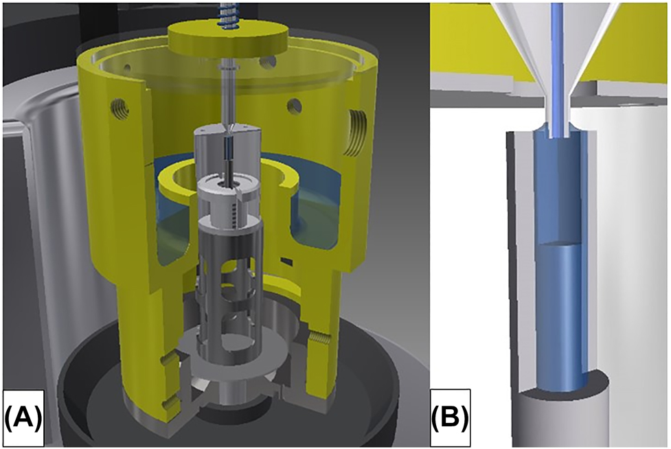
Gravimetric setup at METAS.
(A) Weighing zone on the balance of microflow facility showing outlet needle and beaker with cover. (B) Insight into the contact of the outlet needle in the capillary.
Gravimetric setup at RISE
The gravimetric method at RISE consists of collecting the water in a beaker on the balance with a capacity of 10.1 g (Mettler Toledo XPR10) with the tip of the needle immersed into the water and covered by a layer of paraffin oil to reduce the evaporation rate (Figure 2A) [15]. The temperature is measured by a type K thermocouples at various points in the measurement setup, and the ambient conditions in the laboratory and the in the measurement setup are also logged. Careful preparation of the beaker (inner diameter 15.430 mm and height 53 mm) consists of filling 10 mm with water and then adding 5 mm of paraffin oil (CAS 8012-95-1). An oil layer of at least 4 mm is necessary to drastically reduce the evaporation rate. Thus, the beaker has a final weight of about 4.4 g, which allows up to 5.7 g of water to be collected. Another important aspect is to place the needle approximately in the middle of the water below the oil layer using a traverse system (Figure 2B) prior to the measurement. If the needle is placed too close to the bottom of the beaker respectively to the oil layer, the water delivered through the needle can exert a directional force on the scale respectively cause interaction with the oil layer. The buoyancy of the needle must be taken into account in the measurements (filling process). The outer diameter of the needle used is 0.908 mm (20 G) and each increase of the filling level in the beaker leads to a buoyancy correction of 0.000636 mL/mm or a buoyancy correction factor of 0.996598. The corresponding corrected weight value can then be calculated by means of the actual temperature dependent water density.
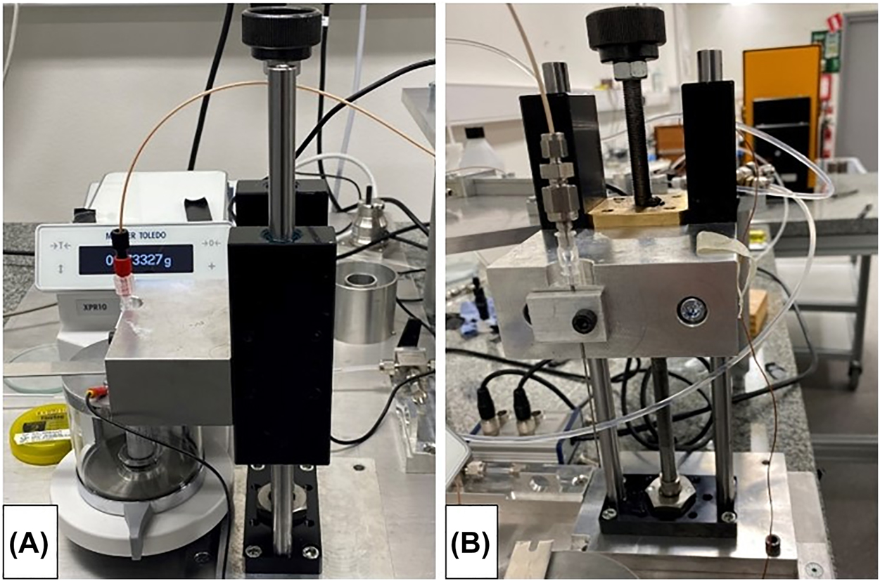
Gravimetric setup at RISE.
(A) Weighing scale with beaker and closed glass draft shield (aluminium draft shield cover and grounding cable). (B) Detailed view of the traverse system (including needle holder).
Front track at IPQ
The front track method consists of measuring the position of the meniscus of a liquid-air interface in a capillary as a function of time. The data of the position and time allows to calculate the speed of the meniscus and by multiplying with the cross section of the capillary to obtain the flow rate as a function of time.
The measurement setup is shown in Figure 3. The insulin pump (1, blue rectangle) is connected by a polypropylene capillary tube (2) to a glass capillary tube (3), where a LED lamp (4) illuminates the capillary through a translucid paper (5) with diffused light. The high speed camera (7) is positioned by checking the field of view (8) using telecentric lenses in order to get the meniscus on the right side of its field of view. The thermometer (6) measures the temperature of the water contained in a beaker placed near the glass capillary tube assuming that the water temperature in the capillary does not vary more than 0.5 °C during the measurement under ambient conditions of (20 ± 3) °C [15]. No temperature sensor can be fixed inside the capillary and therefore the measurement of the temperature is done indirectly in a beaker assuming that this water has the same temperature as the water inside the capillary.
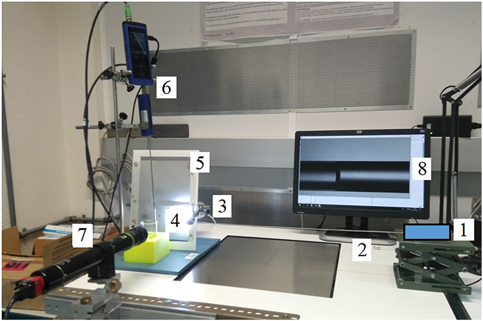
Front track measurement setup at IPQ.
(1) Insulin pump, (2) polypropylene capillary, (3) glass capillary, (4) LED lamp, (5) translucid paper, (6) thermometer, (7) camera, (8) display of field of view.
Measurements were performed using three different glass capillary tubes, one with an internal diameter of 1.15 mm and two others with internal diameters of 0.5 mm and different coatings. The coating of a capillary with a hydrophobic solution acts as friction reducer, decreases the inner volume variability and liquid retention and therefore leads to a more stable meniscus reading. The inner diameter of the capillaries were determined by an in house gravimetric method [19].
Gravimetric setup at DTI
The gravimetric method at DTI consists of a beaker on a scale with microgram resolution, where the tip of the tubing is immersed into the water (Figure 4). By covering the water by a layer of paraffin oil the evaporation rate can be reduced to about 0.2 μL/h [8, 15] and the related uncertainty to less than 0.05 μL/h. The scale is placed on granite table to guarantee a vibration-free base. The setup is in an isolation chamber for improved temperature stability, and furthermore the laboratory itself is temperature controlled. Correction factors for the buoyancy of the displaced air, buoyancy of the displaced water by the needle, the evaporation, and capillary forces are included in the flow rate calculation. The lowest flow rate being measured is about 1 μL/h. The domination contribution to the uncertainty at the lowest flow rate (1 μL/h) is related to the evaporation rate (about ±0.07 μL/h). At slightly higher flow rates (10 μL/h), short-term temperature variations and the uncertainty on the weighing become more significant (both contributions depend on the measuring time). At even higher flow rates, sticking effects dominate and limit the accuracy to about 0.5%.
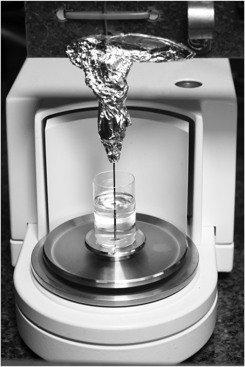
Gravimetric setup at DTI. Weighing scale with a glass beaker and the immersed needle in water with an oil layer on top of it.
Front track at THL
The front track method consists of measuring the position of the meniscus of a liquid-air interface in a capillary as a function of time. The data of the position and time allows to calculate the speed of the meniscus and by multiplying with the cross section of the capillary to obtain the flow rate as a function of time. The measurement setup uses high precision capillaries (0.15–1 mm inner diameter) in combination with a high-speed camera and telecentric lenses (Figure 5) [9, 10, 15]. Die Uncertainty contribution from the diameter and therefore from the cross section is constant independent of flow rate and averaging time. The other contributions depend on the flow rate and the averaging time [10]. The alignment of the capillary is performed by adjustable capillary holders on a linear stage. Acquisition times up to 167 s are possible by using different inner diameters of the capillaries and different magnifications of the measuring lenses.
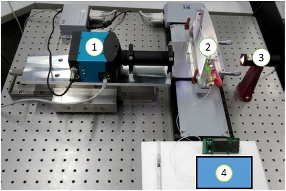
Front track measurement setup at THL.
(1) high-speed camera, (2) capillary, (3) light source with a translucid paper and (4) the insulin pump.
Micro PIV at UoS
The setup of the micro particle image velocimetry (µ-PIV) consisted of a microfluidic device on an inverted microscope (Axio Vert.A1, Zeiss) used with a 20X objective and a CCD camera (Teledyne Dalsa Genie C, Stemmer Imaging) (Figure 6A). Microfluidic devices were fabricated in transparent polydimethylsiloxane (PDMS) and bonded on glass coverslips to allow for high imaging resolution (Figure 6A inset). The device geometry consisted of a serpentine channel with a rectangular cross-section (height of 20 µm and width of 70 µm). A PTFE tube was connected to the inlet of the device and a pressure system (MFCS, Fluigent) was used to prime the device microchannel with micro beads suspended in water (1 µm diameter Styrofoam micro beads, Polysciences). Once the microchannel was completely filled with the bead solution, the tubing was disconnected from the pressure system and attached to the Insulin pump taking care not to generate air bubbles. Collections of images of the bead solution flowing in the microchannel (Figure 6B) are taken at frequencies between 100 and 500 Hz. These sets of images were then processed to obtain the velocities of individual beads (Figure 6C). The flowrate was calculated by modelling the parabolic velocity profile across the width of the channel (Figure 6D).
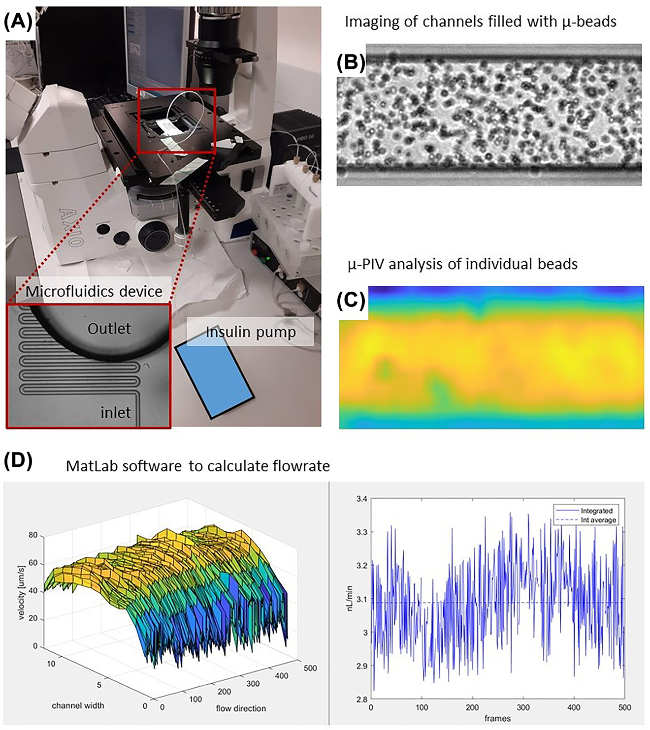
µ-PIV setup at Strathclyde University.
(A) A microfluidic device mounted on the inverted microscope with a CCD camera. The inset shows a magnification of the microchannel of the device. (B) Typical distribution of microbeads in the channel captured by the CCD camera. (C) Velocity distribution of individual µ-beads. (D) Plot of the parabolic flow profile under the field of view and its temporal evolution.
Results and discussion
Mechanism of delivering discrete doses
The calibration of an insulin pump using different measurement and analysis methods is discussed in this chapter to highlight some issues that should be considered in order to accurately calibrate the average basal rate (flow rate) and not to affect the calibration result with systematic errors occurring from analysis artefacts or instabilities in the measurement setup. As mentioned in the introduction, the pump mechanism of the insulin pump consist of a stepper motor that moves the plunger in one or more steps, which pushes forward the piston in the container and delivers a discrete dose of insulin in a given cycle time. The insulin pump investigated has the following discrete doses and cycle times depending on the basal rate setting, as shown in Table 1.
Discrete doses and cycle times for different basal rates of the insulin pump. For convenience, the flow rate in μL/h and the corresponding Basal rate in U/h are listed below. The insulin concentration is usually 100 U/mL.
| Flow rate (μL/h) | Basal rate (U/h) | Discrete dose (nL) | Cycle time (min) |
|---|---|---|---|
| 10.00 | 1.000 | 500 | 3.0 |
| 6.00 | 0.600 | 250 | 2.5 |
| 3.00 | 0.300 | 250 | 5.0 |
| 1.00 | 0.100 | 250 | 15.0 |
| 0.25 | 0.025 | 250 | 60.0 |
The delivery of discrete doses is visible in the raw data of the gravimetric method and the optical front track method, as shown in Figure 7. The weight increase of the gravimetric method shows a significant increase followed by a flattening of the curve before the delivery of the next dose (Figure 7, black line). The same behaviour is observed for the front track methods, shown as blue and red lines. The red line is discontinuous because the optical front track method at THL is limited to a measurement time of 167 s and the gaps are caused by the time needed to transfer the images from the high-speed camera to the PC. Nevertheless, the increase of the position for a dose can be calculated from the positions prior the increase. The blue line representing the position data of the optical front track method at IPQ shows step increases that are heavily smoothed out. This is due to the fact that the tubing is not very stiff and the pressure wave caused by the dose is absorbed by the tubing, resulting in a very smooth increase in position due to pressure relaxation. Nevertheless, the single doses can be identified by the wave-like increase in position.
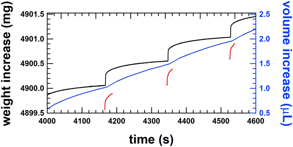
Smooth step increase of the weight of single shots of the order of 500 nL at a cycle time of 3 min for a flow rate of 10 μL/h or 1.0 U/h measured by the gravimetric setup at METAS (black line), by the front track setup at IPQ (blue line) and by the front track setup at THL (red line).
Linear regression analyzing method
Linear regression is often used to determine the mass flow rate from gravimetric weighing data. For linear regression, a fixed time window is chosen and by increasing the start time of this fixed time window by time steps of the corresponding data, the moving average of the flow rate can be followed over time. Further details of this procedure are beyond the scope of this paper and can be found in references [17, 20]. It is also applicable for weight increases that have similar characteristics to a step function. The choice of a short time window allows a detailed investigation of the flow rate evolution over time. Figure 8 shows an example with a fitting window of 30 s at a flow rate of 6 μL/h (black line). The weight increase is represented by the peak value of the flow rate and the flattening of the curve results in a decrease of the flow rate. The amplitude of the peak and the decrease in flow rate depend on the stiffness of the tubing in the setup which may or may not smooth the weight increase. In any case, the average flow rate will remain the same, but the profile of the instantaneous flow rate might be different in amplitude, but not in frequency. The same features are observed by the μ-PIV method, where consecutive images of the particle positions are analysed to determine the flow profile through the channel and calculate the average flow rate in time frames of 5 s (Figure 8, blue line).
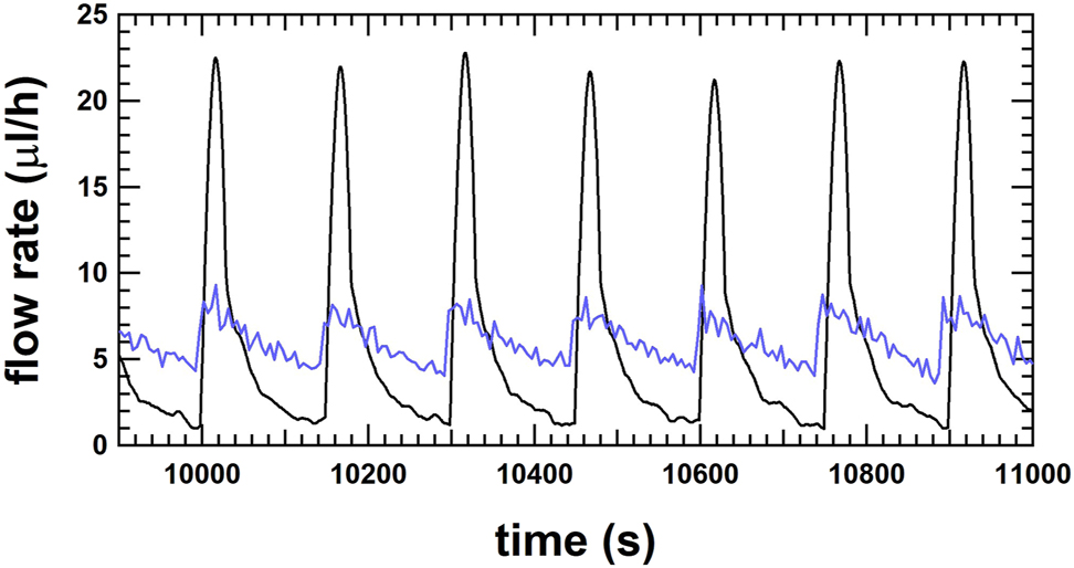
Flow rate as a function of time for the gravimetric method at RISE with a fit window of 30 s (black line) and for the μ-PIV method at UoS with an average time of 5 s (blue line) for the flow rate at 6 μL/h.
The cycle time of the discrete doses is an important time constant for calculating the average flow rate of such smooth step functions. The average flow rate must be averaged over a time window which is an integer multiple of this cycle time to avoid accounting for an artefact from the analysis method. To investigate this effect, linear regression for flow rate determination has been applied to a complete weighing data set at 10 μL/h (cycle time 180 s; only a selection of the data is shown in Figure 7). Table 2 shows the deviations of the set flow rate from the reference flow rate for different linear regressions fitting windows and different averaging time frames. Cells marked in red show large deviations caused by the time frame for averaging not being an integer multiple of the cycle time. Cells marked green show the consistent results when the fitting window is an integer multiple of the cycle time and the time frame for averaging is at least ten times the cycle time. The results are even consistent with the result where the time frame for averaging is 17,000 s. This example clearly shows that it would be advantageous to choose the fitting window being five times the cycle time and the time frame for averaging with at least ten times the cycle time of the delivery of the single doses in order to determine a representative result of the calibrated average flow rate of the insulin pump.
Artefact arising from a fit window not being a multiple integer of the cycle time. Strong deviations are found for improper fit windows with the linear regression method for the flow rate determination. The measurement uncertainty of the results is 0.7%. Data taken from the gravimetric measurement at 10 μL/h (1.0 U/h) at METAS – a short section is shown in Figure 7.
| # Cycle time for average | Start of average (s) | Time frame for average (s) | Deviation (fit window 3,600 s) (%) | Deviation (fit window 1,800 s) (%) | Deviation (fit window 900 s) (%) | Deviation (fit window 180 s) (%) | Deviation (fit window 30 s) (%) | Deviation (fit window 10 s) (%) |
|---|---|---|---|---|---|---|---|---|
| 94.4 | 3,975 | 17,000 | 1.06 | 0.91 | 0.78 | 0.60 | 0.27 | 0.27 |
| 20.0 | 3,975 | 3,600 | 0.33 | 0.41 | 0.39 | 0.28 | 0.18 | 0.19 |
| 15.0 | 3,975 | 2,700 | 0.76 | 0.70 | 0.66 | 0.51 | 0.45 | 0.45 |
| 10.0 | 3,975 | 1800 | 1.02 | 1.05 | 0.84 | 0.53 | 0.49 | 0.50 |
| 5.0 | 3,975 | 900 | 1.33 | 1.03 | 0.53 | −0.07 | −0.42 | −0.41 |
| 4.4 | 3,975 | 800 | 1.38 | 1.03 | 0.22 | −2.57 | −8.66 | −8.80 |
| 4.0 | 3,975 | 720 | 1.42 | 1.02 | 0.11 | −1.01 | −1.37 | −1.35 |
| 3.3 | 3,975 | 600 | 1.50 | 1.07 | −0.30 | −4.03 | −13.11 | −13.29 |
| 2.0 | 3,975 | 360 | 1.65 | 1.05 | −0.41 | −2.22 | −2.74 | −2.72 |
| 1.5 | 3,975 | 270 | 1.72 | 1.07 | −0.39 | −7.68 | −21.49 | −21.79 |
| 1.0 | 3,975 | 180 | 1.75 | 0.93 | 0.19 | −3.07 | −3.65 | −3.54 |
Discrete dose analysis method
The method described in the standard IEC 60601-2-24:2012 – Clause 201.12.1.104 [4] analyses the discrete volumes of the single doses at a constant cycle time. The method used in this work to analyse the discrete doses is very similar, except that the constant cycle time is replaced by the time stamps that identify the step increase in weight for the gravimetric method or the step increase in position for the front track method. The data of the gravimetric method are used to explain the discrete dose analysis method. First, the times of the step increase must be determined by identifying the local maxima in the slope of the curve of the weighing data. The slope of the curve of the weighing data (Figure 9, black line) has been calculated using the linear regression method over a fitting window of 2 s, as shown in Figure 9 (green line). The local maxima of the gradient indicate the times of the step increase, whereby the weight value in the gradient is represented by the green diamond. To calculate the step increase, the weight values prior to the increase must be identified. Therefore, the weight values from −15 to −10 s are averaged with respect to the time stamp of the local maxima in order to reduce the measurement noise. These averaged values are shown as red circles in Figure 9 and are used to determine the weight increment of the single doses by subtracting two consecutive values. At the same time, the corresponding cycle time is also determined and analyzed for irregularities. The histogram of the weight increments is shown in Figure 10, where the average of the discrete dose volume is 496.6 nL with a standard deviation of 21.2 nL, resulting in a deviation of +0.69%. Furthermore, the corresponding cycle times of the discrete doses range between 179.80 and 180.30 s with a mean value of 180.00 s. This analysis method also allows artefacts of the measurement setup to be detected. An example is a change in capillary force on the needle immersed in water, where the force on the balance suddenly changes, causing a sharp increase or decrease of the weight value. The weight increment does not correspond to a discrete dose and the time between two consecutive weight value increments does not correspond to the estimated cycle time. This discrete dose analysis method also makes it possible to detect irregularities from an insulin pump with its infusion set. However, the stabilization time of the measurement setup must comply with the requirements in order not to misinterpret irregularities at the beginning of the measurements.
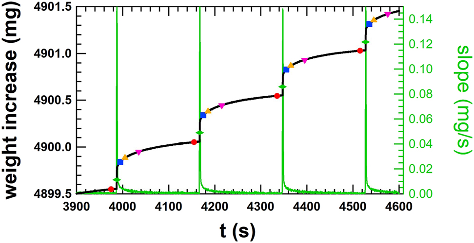
Smooth step increase of the weight of single doses of the order of 500 nL at cycle times of 180 s for a flow rate of 10 μL/h or 1.0 U/h (black line). Average of weight values for 5 s prior to the increase (red circle), in the step increase (green diamond – +12 s), after the step increase (blue square – +20 s, orange triangle up – +30 s, pink triangle down – +60 s). The slope of the step increase of weight for finding the local maxima (green line, right axis) is shown and corresponds to the time of the green diamonds. Data taken from the gravimetric measurement at 10 μL/h (1.0 U/h) at METAS – same data as Figure 7.
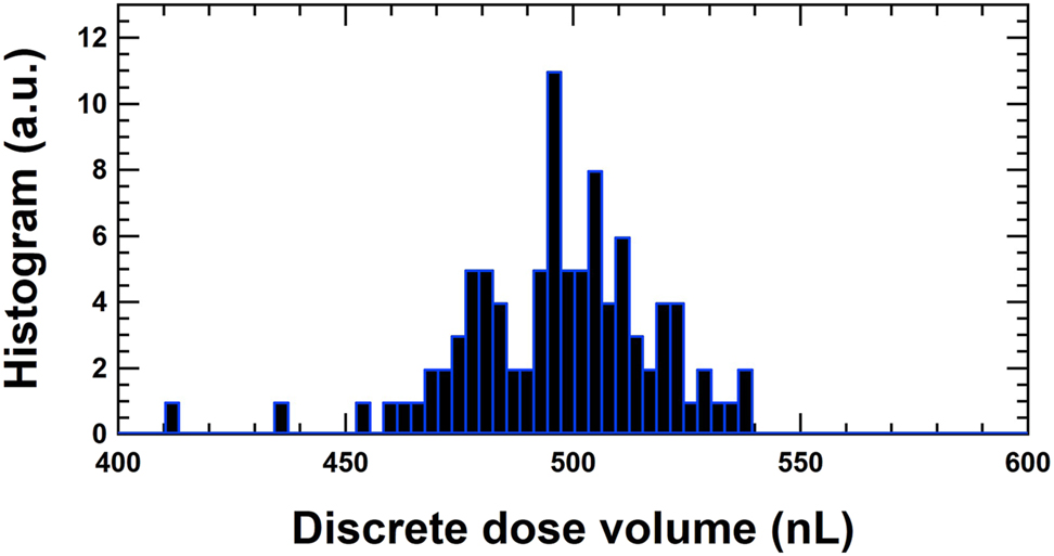
The dose volumes at 10 μL/h for the measurements at METAS are represented in a histogram. The average of the dose volumes from 3,975 to 20,895 s is 496.6 nL leading to a deviation of +0.69%. The corresponding cycle times of the discrete doses are between 179.80 and 180.30 s with an average of 180.00 s.
Another issue arises from the starting point of the discrete dose analysis method, which is even more important for the similar method described in the standard IEC 60601-2-24:2012, where no requirements for the starting point of the data analysis are specified and a fixed cycle time is applied. Several starting points are chosen, whereby the starting point for the discrete dose analysis lies prior to the increase (Figure 9, red circle), whilst the step increase (green diamond – +12 s) or after the step increase (blue square – +20 s; orange triangle up – +30 s; pink triangle down – +60 s). The average over the discrete dose volumes has always been calculated over the same acquisition time in to obtain the average over the same number of discrete doses. The results are listed in Table 3 and show no significant dependence on the starting point for both the discrete dose analysis and the method according to IEC 60601-2-24:2012. It is also important to note that for this data set, the deviations of both methods are consistent and only a minor variation is observed. Averaging the weight values over 5 s slightly differs the results from the method in IEC 60601-2-24:2012, where only single weight values are taken for the analysis without reducing the reading noise of the balance. However, the difference is negligible compared to the measurement uncertainty.
Calibration of the average volume dose for a flow rate at 10 μL/h with the gravimetric method and the discrete volume analysis method for different starting points prior, during and after the step increase of the weight. Additionally, the results with the method described in the standard IEC 60601-2-24 are listed. Deviation is calculated according to VIM [21]: (set value – ref value)/ref value ∗100%.
| Set dose volume (nL) | Reference volume (nL) | Stabilisation time (s) | Starting point Figure 9 | Acquisition time (s) | # shot cycle | Deviation (%) | Deviation by the IEC method (%) | Uncertainty (%) |
|---|---|---|---|---|---|---|---|---|
| 500 | 496.56 | 3,975 | Red circle | 16,920 | 94 | 0.68| | 0.83 | 0.70 |
| 500 | 496.46 | 3,987 | Green diamond | 16,920 | 94 | 0.71 | 0.84 | 0.70 |
| 500 | 496.35 | 3,995 | Blue square | 16,920 | 94 | 0.74 | 0.83 | 0.70 |
| 500 | 496.32 | 4,005 | Orange triangle up | 16,920 | 94 | 0.74 | 0.83 | 0.70 |
| 500 | 496.28 | 4,035 | Pink triangle down | 16,920 | 94 | 0.75 | 0.82 | 0.70 |
Calibration results of the insulin pump with the gravimetric and optical methods
With the knowledge of analyzing the flow rate in a time window that is an integer multiple of the dose cycle time, the measurement data collected with the gravimetric and optical setups for insulin pump delivery have been analyzed, shown in Figure 11 and listed in Table 4.
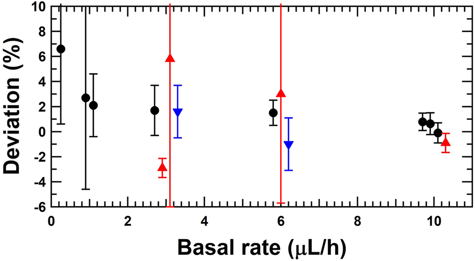
Deviation of the set basal rate with respect to the reference flow rate of the insulin pump for the gravimetric method (black circles), the front tracking method (red triangle up) and the micro PIV (blue triangle down).
Calibration results of the insulin pump at different basal rates by gravimetric and optical methods. Deviation is calculated according to VIM [21]: (set value – ref value)/ref value ∗100%.
| Set basal rate (μL/h) | Reference flow rate (μL/h) | Stabilisation time (s) | Acquisition time (s) | # shot cycle | Deviation (%) | Uncertainty (%) | Method | Partner |
|---|---|---|---|---|---|---|---|---|
| 10 | 9.931 | 3,975 | 16,920 | 94.0 | 0.69 | 0.70 | Gravimetric – discrete doses | METAS |
| 10 | 9.923 | 3,975 | 17,000 | 94.4 | 0.78 | 0.70 | Gravimetric – linear regression. | METAS |
| 10 | 9.937 | 0 | 216,000 | 1,200.0 | 0.63 | 0.87 | Gravimetric – discrete doses | DTI |
| 10 | 10.010 | 3,600 | 82,800 | 460.0 | −0.10 | 0.80 | Gravimetric – linear regression | RISE |
| 10 | 10.090 | 4,885 | 1,620 | 9.0 | −0.90 | 0.76 | Optical front track | THL |
| 6 | 5.910 | 3,600 | 82,800 | 460.0 | 1.5 | 1.0 | Gravimetric – linear regression | RISE |
| 6 | 5.825 | 600 | 1,080 | 6.0 | 3.0 | 8.7 | Optical front track | IPQ |
| 6 | 6.063 | 9,590 | 1,500 | 10.0 | −1.0 | 2.1 | Micro PIV | Strathclyde |
| 3 | 2.835 | 600 | 1,620 | 9.0 | 5.8 | 11.8 | Optical front track | IPQ |
| 3 | 2.950 | 3,600 | 82,800 | 460.0 | 1.7 | 2.0 | Gravimetric – linear regression | RISE |
| 3 | 2.951 | 4,070 | 7,950 | 26.5 | 1.6 | 2.1 | Micro PIV | Strathclyde |
| 3 | 3.090 | 3,300 | 2,700 | 9.0 | −2.9 | 0.76 | Optical front track | THL |
| 1 | 0.979 | 3,600 | 82,800 | 460.0 | 2.1 | 2.5 | Gravimetric – linear regression | RISE |
| 1 | 0.974 | 0 | 432,000 | 2,400.0 | 2.7 | 7.3 | Gravimetric – discrete doses | DTI |
| 0.25 | 0.23 | 7,200 | 79,200 | 440.0 | 6.6 | 6.0 | Gravimetric – linear regression | RISE |
All the results are within ±7%. There are some variations in the calibration results, which can be explained by long-term fluctuations in the basal rate due to the pumping mechanism. The measurement results for a period of more than 60 h at 10 μL/h are shown in Figure 12. These long-term fluctuations are due to spindle rotation of the pumping mechanism. Unfortunately, the spindle increment per rotation is not known for this insulin pump, but each spindle revolution cycle causes the periodicity of these long-term fluctuations. This feature is common for this kind of pumping mechanism and is also observed for syringe pumps, which are also based on a rotating spindle to move the plunger forward. Therefore, for short measurement times in the order of several hours, the calibrated basal rates may always show some variation. Even if the measurement time is extended the long-term fluctuations can be smoothed, but remain observable. The reproducibility measurements have been performed at DTI at a basal rate of 10 μL/h and a measurement time of at least 16 h, as listed in Table 5.
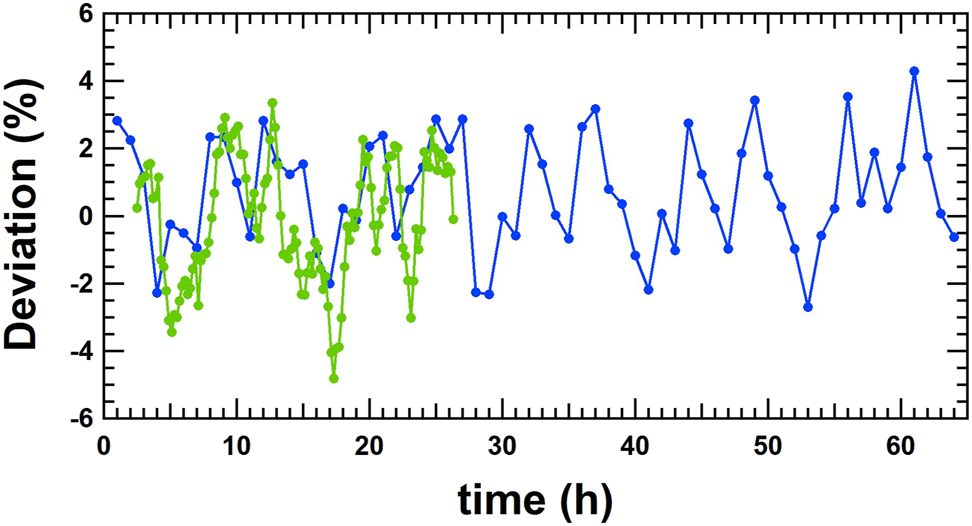
Long term measurements at 10 μL/h performed at DTI (blue line) and RISE (green line). Each measurement point is an average of 1 h (20 discrete doses). All the deviations are within ±5%.
Reproducibility measurements at a basal rate of 10 μL/h performed at DTI with the gravimetric method. Deviation is calculated according to VIM [21]: (set value – ref value)/ref value ∗100%.
| Set basal rate (μL/h) | Reference flow rate (μL/h) | Stabilisation time (s) | Acquisition time (s) | # shot cycle | Deviation (%) | Uncertainty (%) | Method | Partner |
|---|---|---|---|---|---|---|---|---|
| 10 | 9.937 | 0 | 216,000 | 1,200.0 | −0.2 | 0.9 | Gravimetric – discrete doses | DTI |
| 10 | 9.857 | 0 | 79,200 | 440.0 | −0.8 | 1.9 | Gravimetric – discrete doses | DTI |
| 10 | 9.908 | 0 | 86,400 | 480.0 | −0.7 | 1.8 | Gravimetric – discrete doses | DTI |
| 10 | 9.977 | 0 | 57,600 | 320.0 | −1.4 | 1.7 | Gravimetric – discrete doses | DTI |
There are no requirements for the accuracy of the insulin pumps stated in the IEC 60601-2-24:2012. However, most of the manufacturers state an accuracy of ±5% in their manual [22].
Bolus calibration results with the gravimetric and optical methods
In addition to the calibration of the basal rate of the insulin pump, the calibration of the delivery of different boluses is also important and has been performed according to the gravimetric method described in the standards for the calibration of syringe(s) and glass ware [23, 24] or with the actual gravimetric setup, with the needle immersed into water with a layer of oil on top. The sizes of the boluses were 0.25, 1.0, 3.0, 6.0 and 10.0 μL, and the repeatability of the calibration of the boluses was taken into account by performing at least five measurements. The deviations of the boluses are listed in Table 6 and presented in Figure 13.
Calibration of several boluses. Deviation and measurement uncertainty including the repeatability of at least 5 measurements are presented.
| Set bolus target (μL) | Deviation IPQ (%) | Deviation RISE (%) | Deviation DTI (%) |
|---|---|---|---|
| 10 | (1.5 ± 3.2) | (0.0 ± 3.8) | (1.1 ± 5.5) |
| 6 | (−8.0 ± 4.2) | (−1.1 ± 3.6) | (2.5 ± 4.4) |
| 3 | (−0.5 ± 6.6) | (−1.3 ± 3.5) | (3.3 ± 2.9) |
| 1 | (9.1 ± 14.4) | (−6.0 ± 6.4) | – |
| 0.25 | (11.0 ± 8.0) | (−3.0 ± 12.6) | – |
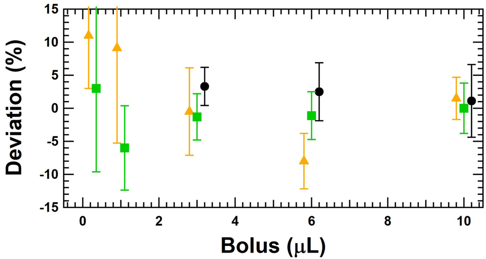
Calibration of several boluses being 0.25, 1.0, 3.0, 6.0 and 10.0 μL with the gravimetric method at DTI (black circles), RISE (green squares) and IPQ (orange triangle). The measurement uncertainty includes the repeatability of at least five measurements.
The results are all within ±11% and for some bolus sizes (3 and 10 µL) the consistency is very good. It is important to note that the measurement of the bolus size is also influenced by the effect of the spindle rotation mechanism. This means that the results are influenced by the different positions of the piston inside the container but also by the long-term fluctuations. The variation of the results in Figure 13 can therefore be partially explained by this fact, although it cannot be excluded that the gravimetric measurement methods do not show any variations in the determination of the boluses. It would be advisable to determine the bolus size at different positions of the piston in the container in order to somehow average out the long-term fluctuation caused by the pumping mechanism.
Conclusions
The gravimetric and optical methods described in this paper allow a detailed analysis of the delivery mechanism of insulin pumps delivering discrete doses at given cycle times. The discrete dose analysis method allows for detailed follow-up of dose cycle time and delivered doses as a function of time, and to investigate the short- and long-term performance of insulin pumps. Furthermore, it has been shown that basal rate determination by means of the widely used linear regression method for flow rate determination with an additional requirement is also applicable. It is advantageous to choose the fitting window to be five times the cycle time and the averaging time frame to be at least ten times the cycle time of the delivery of the single doses in order to obtain a representative result for the calibrated average flow rate of the insulin pump.
The discrete dose analysis method is also suitable for the determining bolus sizes. Due to the long-term fluctuations caused by the pumping mechanism, it is advisable to determine the bolus size at different positions of the piston in the container in order to somehow compensate these long-term fluctuations.
These calibration measurements show that this discrete dose analyzing method also allows to detect irregularities from an insulin pump with its infusion set. However, the requirements of the measurement setup, such as the stabilization time or the time frame for calculating an average value, must be respected in order not to misinterpret irregularities or malfunctions of the insulin pump.
Funding source: European Metrology Programme for Innovation and Research
Award Identifier / Grant number: 18HLT08 MEDDII
-
Research funding: This project 18HLT08 MEDDII has received funding from the EMPIR programme co-financed by the Participating States and from the European Union’s Horizon 2020 research and innovation programme.
-
Author contributions: All authors have accepted responsibility for the entire content of this manuscript and approved its submission.
-
Competing interests: Authors state no conflict of interest.
-
Informed consent: Informed consent was obtained from all individuals included in this study.
-
Ethical approval: Not applicable.
References
1. Thornton, J, Sakhrani, V. How lubricant choice affects dose accuracy in insulin pumps. ONdrugDelivery Magazine 2017;32–6.Search in Google Scholar
2. Jahn, LG, Capurro, JJ, Levy, BL. Comparative dose accuracy of durable and patch insulin infusion pumps. J Diabetes Sci Technol 2013;7:1011–20. https://doi.org/10.1177/193229681300700425.Search in Google Scholar PubMed PubMed Central
3. Dumont-Fillon, D, Tahriou, H, Conan, C, Chappel, E. Insulin micropump with embedded pressure sensors for failure detection and delivery of accurate monitoring. Micromachines 2014;5:1161–72. https://doi.org/10.3390/mi5041161.Search in Google Scholar
4. IEC 60601-2-24:2012. Medical electrical equipment – part 2-24: particular requirements for the basic safety and essential performance of infusion pumps and controllers; 2012.Search in Google Scholar
5. Bissig, H, Tschannen, M, de Huu, M. Traceability of pulsed flow rates consisting of constant delivered volumes at given time interval. Flow Meas Instrum 2020;73:101729. https://doi.org/10.1016/j.flowmeasinst.2020.101729.Search in Google Scholar
6. Zisser, H, Breton, M, Dassau, E, Markova, K, Bevier, W, Seborg, D, et al.. Novel methodology to determine the accuracy of the OmniPod insulin pump: a key component of the artificial pancreas system. J Diabetes Sci Technol 2011;5:1509–18. https://doi.org/10.1177/193229681100500627.Search in Google Scholar PubMed PubMed Central
7. Zisser, H. Insulin pump (dose-to-dose) accuracy: what does it mean and when is it important? J Diabetes Sci Technol 2014;8:1142–4. https://doi.org/10.1177/1932296814548216.Search in Google Scholar PubMed PubMed Central
8. Bissig, H, Petter, HT, Lucas, P, Batista, E, Filipe, E, Almeida, N, et al.. Primary standards for measuring flow rates from 100 nl/min to 1 ml/min – gravimetric principle. Biomed Tech 2015;60:301–16. https://doi.org/10.1515/bmt-2014-0145.Search in Google Scholar PubMed
9. Ahrens, M, Nestler, B, Klein, S, Lucas, P, Petter, HT, Damiani, C. An experimental setup for traceable measurement and calibration of liquid flow rates down to 5 nl/min. Biomed Tech 2015;60:337–45. https://doi.org/10.1515/bmt-2014-0153.Search in Google Scholar PubMed
10. Ahrens, M, Klein, S, Nestler, B, Damiani, C. Design and uncertainty assessment of a setup for calibration of microfluidic devices down to 5 nL min−1. Meas Sci Technol 2014;25:015301. https://doi.org/10.1088/0957-0233/25/1/015301.Search in Google Scholar
11. Ochoa, M, Ziaie, B. Analysis of novel methods to determine the accuracy of the Omnipod insulin pump: a key component of the artificial pancreas system. J Diabetes Sci Technol 2011;5:1519–20. https://doi.org/10.1177/193229681100500628.Search in Google Scholar PubMed PubMed Central
12. Oliver, N, Reddy, M, Marriott, C, Walker, T, Heinemann, L. Open source automated insulin delivery: addressing the challenge. NPJ Digit Med 2019;2:124–8. https://doi.org/10.1038/s41746-019-0202-1.Search in Google Scholar PubMed PubMed Central
13. American Diabetes Association. 7 Diabetes technology: standards of medical care in diabetes – 2019. Diabetes Care 2019;42:71–80. https://doi.org/10.2337/dc19-s007.Search in Google Scholar PubMed
14. Batista, E, Furtado, A, Pereira, J, Ferreira, M, Bissig, H, Graham, E, et al.. New EMPIR project – Metrology for drug delivery. Flow Meas Instrum 2020;72:101716. https://doi.org/10.1016/j.flowmeasinst.2020.101716.Search in Google Scholar
15. Morgan, J, Graham, E, Gersl, J, Batista, E, Bissig, H, Ogheard, F, et al.. A1.2.5 Calibration methods for measuring the response or delay time of drug delivery devices using Newtonian liquids for flow rates from 5 nL/min to 100 nL/min: EURAMET 18HLT08 MeDDII; 2021. Available from: www.drugmetrology.com.Search in Google Scholar
16. Graham, E, Thiemann, K, Kartmann, S, Batista, E, Bissig, H, Niemann, A, et al.. Ultra-low flow rate measurement techniques. Sensors 2021;18:100279. https://doi.org/10.1016/j.measen.2021.100279.Search in Google Scholar
17. Bissig, H, Tschannen, M, de Huu, M. Micro-flow facility for traceability in steady and pulsating flow. Flow Meas Instrum 2015;44:34–42. https://doi.org/10.1016/j.flowmeasinst.2014.11.008.Search in Google Scholar
18. Wright, JD, Schmidt, JW. Reproducibility of liquid micro-flow measurements. In: Proc Flomeko: Lisbon, Portugal; 2019.Search in Google Scholar
19. Batista, E, Alvares, M, Martins, R, Ogheard, F, Gersl, J, Godinho, I. Measurement of internal diameters of capillaries and glass syringes using gravimetric and optical methods for microflow applications. Biomed Eng Biomed Tech 2023;68:29–38.10.1515/bmt-2022-0033Search in Google Scholar PubMed
20. Bissig, H, Tschannen, M, de Huu, M. Recent Innovations in the field of traceable calibration of liquid milli-flow rates with liquids other than water. Sydney, Australia: Proc Flomeko; 2016.Search in Google Scholar
21. JCGM 200:2012. International vocabulary of metrology – Basic and general concepts and associated terms (VIM), 3rd ed; 2012.Search in Google Scholar
22. Freckmann, G, Kamecke, U, Waldenmaier, D, Haug, C, Ziegler, R. Accuracy of bolus and basal rate delivery of different insulin pump systems. Diabetes Technol Therapeut 2019;21:201–8. https://doi.org/10.1089/dia.2018.0376.Search in Google Scholar PubMed PubMed Central
23. ISO 4787:2021. Laboratory glass and plastiv ware – Volumetric instruments – Methods for testing of capacity and for use; 2021.Search in Google Scholar
24. ISO 8655-9:2022 – Piston-operated volumetric apparatus – Part 9: Manually operated precision laboratory syringes. Under Publication; 2022.Search in Google Scholar
© 2022 the author(s), published by De Gruyter, Berlin/Boston
This work is licensed under the Creative Commons Attribution 4.0 International License.
Articles in the same Issue
- Frontmatter
- Guest Editorial
- Medical flow and dosing measurement metrology in drug delivery
- Special Issue Articles
- Metrology in health: challenges and solutions in infusion therapy and diagnostics
- Calibration methods for flow rates down to 5 nL/min and validation methodology
- Measurement of internal diameters of capillaries and glass syringes using gravimetric and optical methods for microflow applications
- In-line measurements of the physical and thermodynamic properties of single and multicomponent liquids
- Assessment of drug delivery devices working at microflow rates
- Calibration of insulin pumps based on discrete doses at given cycle times
- Development of a microfluidic electroosmosis pump on a chip for steady and continuous fluid delivery
- Effect of non-return valves on the time-of-arrival of new medication in a patient after syringe exchange in an infusion set-up
- Holographic PIV/PTV for nano flow rates–A study in the 70 to 200 nL/min range
- Unexpected dosing errors due to air bubbles in infusion lines with and without air filters