Holographic PIV/PTV for nano flow rates–A study in the 70 to 200 nL/min range
-

 ,
,
,
and
,
,
,
and

Abstract
Accurately measuring flow rates is a key requirement in many medical applications such as infusion and drug delivery systems. A major drawback of current systems is the low resolution of the sensors in the low flow rate regime. In this article, we present a method based on Holographic PIV/PTV that has been used for the first time to measure flow rates in the range of a few nL/min. Our method requires a very simple setup that combines lensless holography with particle velocimetry. For flow rates in the 70 to 200 nL/min range, the highest uncertainty was 5.6% (coverage factor k=2). This is an open-source project; the CAD designs and software source code are available at https://github.com/gui-miotto/holovel.
Introduction
Accurately measuring low flow rates is important for many medical applications, such as neonatology where infusion pumps need to precisely deliver very little volume at low flow rates. In an earlier special issue publication from Snijder et al. [1] different methods of measuring low flow rates have been investigated. In this paper, we present a novel approach combining Lensless Digital Holographic Microscopy (LDHM) with particle velocimetry techniques to measure for the first time flow rates in the nL/min range. Previous works [2, 3] have also used holographic particle velocimetry to measure low flow rates, however they relied on microscopes with 60x water-immersed objectives. Our approach, on the other hand, does not use any lenses. Its advantages are simplicity, compactness, and low cost since it is made of just three components: a digital image sensor, a light source, and a transparent flow channel.
Velocimetry techniques are used to measure flow velocities using image sequences of fluids seeded with tracer particles. The ideal tracer particle follows the velocity of its surrounding liquid and does not influence the flow under observation. This requires the particle to be small and neutrally buoyant, meaning the particle has the same density as the liquid [4]. In low Reynolds flows, small neutrally buoyant particles are responsive to the drag forces, therefore minimizing the liquid-to-particle velocity latency [5]. However, particles should be large enough to be reliably imaged and not affected by Brownian motion. Generally, good and consistent visibility is achieved if the particle’s diameter is at least twice the sensor’s pixel size, and Brownian motion is not relevant for particle diameters larger than 1 µm [6].
Two well-known velocimetry techniques are Particle Tracking Velocimetry (PTV) and Particle Image Velocimetry (PIV). PIV calculates velocities from image regions, by dividing the video frames into small patches and estimating the velocity by cross-correlating corresponding patches in successive frames. PTV calculations refer to individual particles by tracking their position across a sequence of frames. Regardless of the method, having good quality images of the flow is essential. Both algorithms can be used to measure flow profiles, but in our study, we are only interested in the total flow rate, which can be calculated as the average of the of the flow components. Since PTV and PIV have different advantages and disadvantages, both algorithms are tested in this paper.
The imaging system presented here is based on the Lensless Digital Holographic Microscopy (LDHM) [7] principle illustrated in Figure 1. The observed object is illuminated by a coherent point source. The object-incident light deviates from its original trajectory due to refraction and, therefore, will interfere with light that travels undisturbed through the transparent media around the object. The wavefront arriving at a screen placed in front of the object exhibits fringe patterns. Those patterns are the result of the interference between the object-refracted light and the undisturbed light, also known as reference light. The photographic recording on the screen is called a hologram. The hologram allows for later reconstruction of the light field present at the moment of the observation. Because the hologram holds information about the amplitude and the phase of the resulting wave, it is possible to recover an object’s three-dimensional geometry from the two-dimensional hologram.

The lensless holographic microscopy principle. The light emitted by a point source is scattered by the objects under observation. The scattered wave interferes with the reference wave, which is the one that did not interact with the objects. The photographic register of the interference pattern between the two waves is called a hologram. A hologram entails information about the magnitude and phase of the wavefront, making it possible to reconstruct the object’s 3D shape.
Lensless holographic microscopy was invented in 1948 by Dennis Garbor [8] as a new microscope principle which is not affected by optical aberrations, since it does not rely on lenses. Back then, the holograms were recorded on photographic plates and reconstructed by re-illuminating them. Nowadays, holograms are recorded with digital image sensors and reconstructed numerically using equations such as the Kirchhoff-Fresnel diffraction formula. This newer variant is more robust and convenient to use.
The LDHM setup is relatively simple; however, certain requirements need to be addressed regarding the image sensor, light source, and object spatial distribution. The sensor must provide a high signal-to-noise ratio and have a small pixel size since these are the main limiting factors to the resolution of the method [9]. The light source must be spatial and temporal coherent to allow for proper interference of the reference and the scattered wave [10]. To achieve a robust numerical reconstruction, the power of the light source must be such that the interference patterns have sufficient intensity and multiple diffraction orders are visible. Finally, the scattered wave needs to be weak in comparison to the reference wave; otherwise, the reconstruction quality will decrease. For our application, the amount of scattered light is small enough as long as the concentration of tracer particles is not too high.
In the following sections, we present more details about our experimental setup and the analysis software. We then estimate the method’s uncertainty with the aid of large amounts of simulated data. Next, we test our method on real experimental data. Finally, we discuss the obtained results and propose ways to further improve the method.
Materials and methods
Our measurement setup consisted of a transparent custom-made straight microfluidic channel, a digital image sensor, and a light source (Figure 2). The liquid flowing through the channel is seeded with neutrally buoyant particles, to make the flow visible to the sensor. Once a video of the flow is recorded, each holographic frame is reconstructed, and the flow rate in the channel is estimated using a velocimetry algorithm.
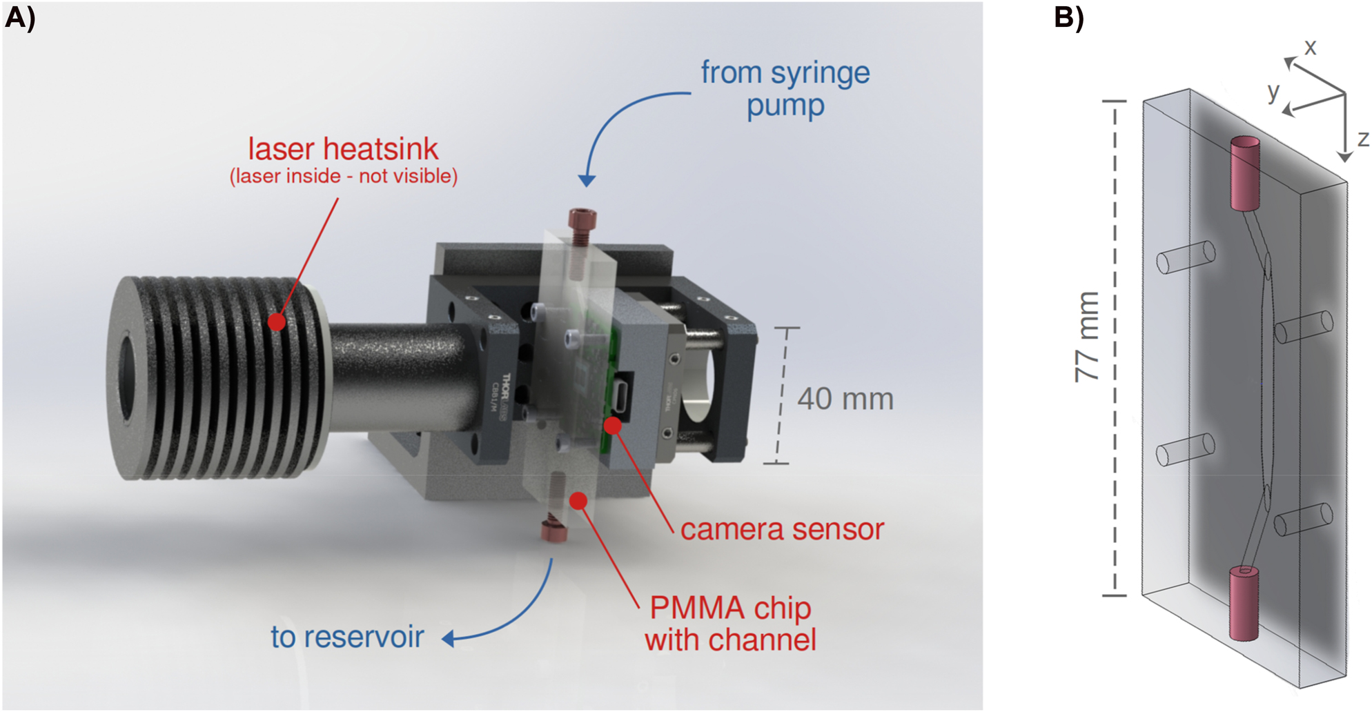
Experimental setup. A) Assembly of the components. Channel is mounted vertically and the flow direction is from top to bottom. B) PMMA chip schematics. Channel is milled on one of the faces of the chip, then sealed with adhesive tape. This face is the one closest to the image sensor. The orientation axis display the convention adopted in this paper: y aligns with the channel’s height, x aligns with the channel’s width, z aligns with the channel’s length, with the flow direction, and with the gravitational acceleration.
Experimental setup
The microfluidic channel was milled into a polymethyl methacrylate (PMMA) block measuring 40 × 8 × 77 mm (W × H × L). The channel itself was designed to be 20 mm long with cross-section dimensions of 1,000 × 30 µm (W × H), which corresponds to an area of 30,000 µm2. The height of the channel is relatively shallow in order to keep the particles close to the sensor to increase their visibility. After fabrication, the channel was polished with plastic polish paste (Xerapol) to remove milling ripples. The ripples, if not removed, diffract too much light, worsening the particle visibility (Figure 3). The precision of our method relies on accurately knowing the cross-sectional area of the channel, therefore, before running the experiments, we optically measured its geometry with focus-variation microscopy (Confovis TOOLinspect, magnification 20x, 275 nm lateral resolution, 300 nm depth resolution). By averaging the area of 2000 cross-sectional profiles, we saw that the channel’s area was in fact 27,893 µm2, 7% smaller than expected (Figure 4). The channel was sealed by applying a microfluidic adhesive tape (3 M Diagnostic Tape 9795R) on the milled side of the PMMA block. The tape was 100 µm thick and consisted of a clear polypropylene film coated with pressure sensitive silicone-based adhesive.
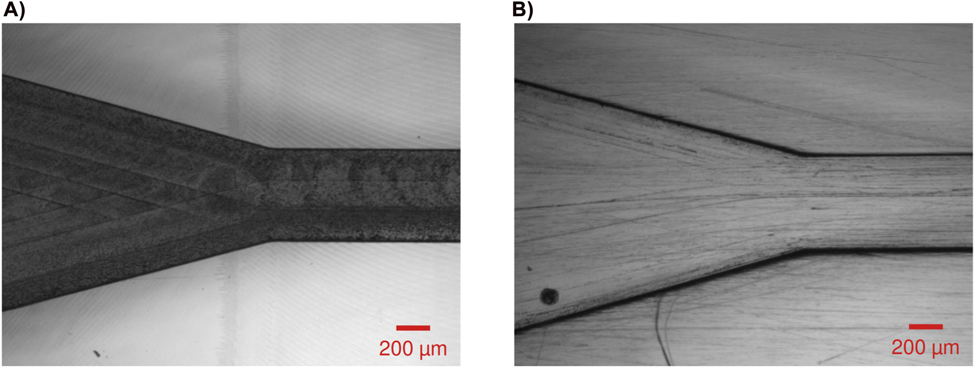
The effects of surface polishing on channel visibility. A) A channel before polishing. B) The same channel after polishing (Images acquired on a lens-based microscope. The channel shown here is not the one used in our measurements).
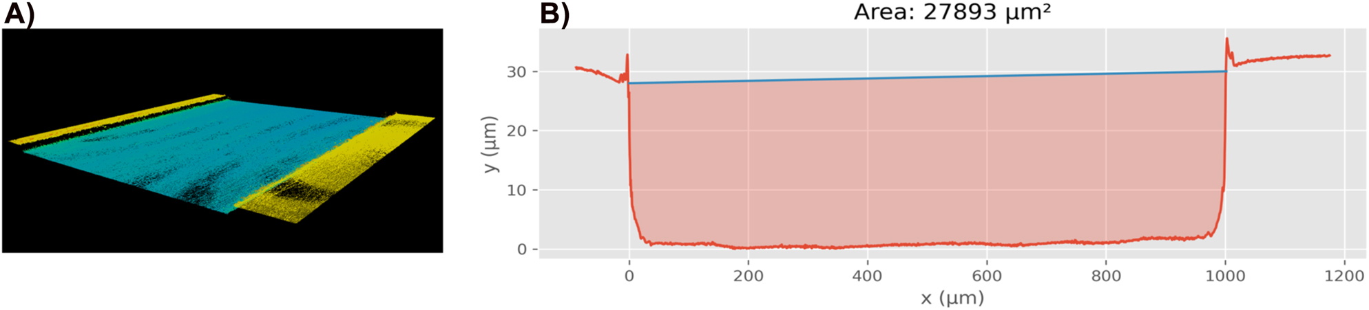
Measurement of the channel’s real geometry using focus-variation microscopy. A) 3D point cloud obtained by the microscope. B) Average channel cross-section (an average of 2000 parallel profiles spread over a channel distance of 700 µm). The spikes near at the border of the channel are not physical, they are artefacts of the imaging method due to reflection on the edges. Also note that the axes are not to scale.
The image sequences were recorded at 10 frames per second using a CMOS sensor (iDS UI-3592LE-C Rev.2). The sensor has 4,912 × 3,684 pixels, where each pixel is a square with a side length of 1.25 µm. Therefore, it was possible to image the full width of the channel and a length of 6.14 mm. The sensor provides RGB images, but they were converted to gray-scale because LDHM is intrinsically monochromatic, therefore the holograms should have a single light intensity channel. The sensor is positioned roughly at the middle of the channel’s length and directly under it. The air gap between the sensor and the channel is less than one mm wide. An 80 mW blue laser diode (PL450B, λ = 450 nm) was used as the light source.
The flow was generated and controlled by a syringe pump (Nemensys Low Pressure, NEM-B101-02 B, 14:1 gear). The syringe used (SETonic P/N 3,010,307) had a total volume of 1 mL for a 6 cm stroke allowing a minimum flow rate of 70 nL/min. The pumped liquid was purified water, seeded with polystyrene (PS) beads measuring 5 µm in diameter, which is large enough to avoid Brownian motion. Before each experiment, the mixture was agitated to make sure that the beads were uniformly distributed in the water. The beads had a density of 1.05 g/cm³, which gave them the tendency to slowly sediment. As shown in Figure 2, the channel was mounted such that the flow is in direction of gravity, therefore this sedimentation has to be accounted for when calculating the flow velocity.
A total of 50 image sequences were recorded, each 12 s long. The sequences were roughly equally distributed among seven different flow rates: 0, 70, 100, 125, 150, 175, and 200 nL/min. To minimize any transient effects, we waited 30 min before recording a new sequence, whenever the pump’s flow rate was altered. The sequences were stored on a hard drive and the data analysis was performed offline.
Simulation
Besides collecting experimental data, we also generated synthetic data by simulation. The product of the simulations were particle trajectories inside a rectangular flow channel. Many sets of trajectories were generated by imposing different total flow rates. The trajectories were then converted to synthetic holographic videos. The objective here is to quantify how well our measurement method is able to estimate the imposed flow rate when processing the synthetic holographic videos. More precisely, the synthetic data was used to estimate the combined standard uncertainty of our measurement method. In comparison to the experimental data, the synthetic data is a reference standard with negligible value uncertainty (u ref ). Which implies that fluid velocity is constant and its value equal to the one imposed to the simulation. The same is not true for the experimental data, for which the real flow rate value can diverge significantly from the flow rate setpoint of the syringe pump for reasons such as the pump’s dosing precision or flaws in the setup (for instance, elasticity in the tubings and leaks in the connections). By using synthetic data, we factor out the measurement error caused by the instabilities of the flow rate during a measurement.
Another advantage of synthetic data is that, once the simulator is built, it is easy to generate high volumes of data. In total 600 videos were generated, 100 for each of the investigated flow rates (70, 100, 125, 150, 175, and 200 nL/min).
To generate the synthetic data, we combined a Computer Fluid Dynamics (CFD) simulator, with a hologram generator. Using the CFD simulator we calculated the flow profile inside the channel for a given flow rate (boundary condition), with which we calculated the trajectory of particles inside the channel. Finally, using the hologram generator, we rendered these trajectories as holographic videos.
The CFD simulations were done using OpenFOAM’s icoFoam [11], which is a single-phase, incompressible, laminar, transient solver. The simulated geometry corresponded to our channel design (1,000 × 30 µm cross-section). The mesh was orthogonal, made only of rectangular cuboids cells measuring 2 × 2 × 20 µm, where the largest dimension is parallel to the flow direction. The walls of the channel received no-slip boundary conditions. The simulation was conducted for 20 ms, which was enough to bring the flow to a steady state. The result of the simulations are velocity profiles as the one shown in Figure 5.

Velocity profile on the cross-section of the channel for a flow rate 100 nL/min. x and y axes are not to scale.
The next step is to calculate the particle trajectories. Approximately 230 particles are visible in each frame, which is similar to the amount in the experimental data. For each new particle that entered the channel, x and y coordinates were randomly sampled from uniform distributions. Using the x-y coordinates, we can get the velocity vz from the simulated flow profile. The other velocity components (vx and vy) are constant and equal to zero, due to the fact that the particles are perfectly following the uniform laminar flow, as observed experimentally at low Reynolds numbers [12]. The simulation recalculates the position of each particle every 0.1 s, which matches the frame rate used in our experiments. From these sequences of positions the particle trajectory is determined.
To transform the trajectories into a sequence of holograms, we used the light scattering routines provided by the Python package HoloPy [13]. The particles were modeled as spheres with a diameter of 5 µm and refractive index of 1.6 (Polystyrene). The holograms have a pixel size of 1.25 µm and dimensions 800 × 2,187 pixels. These specifications also match the conditions of the experimental setup in terms of tracer particle and image sensor. To increase realism, the holograms are then corrupted with random speckle noise and blurred with a Gaussian filter. The result is shown in Figure 6.
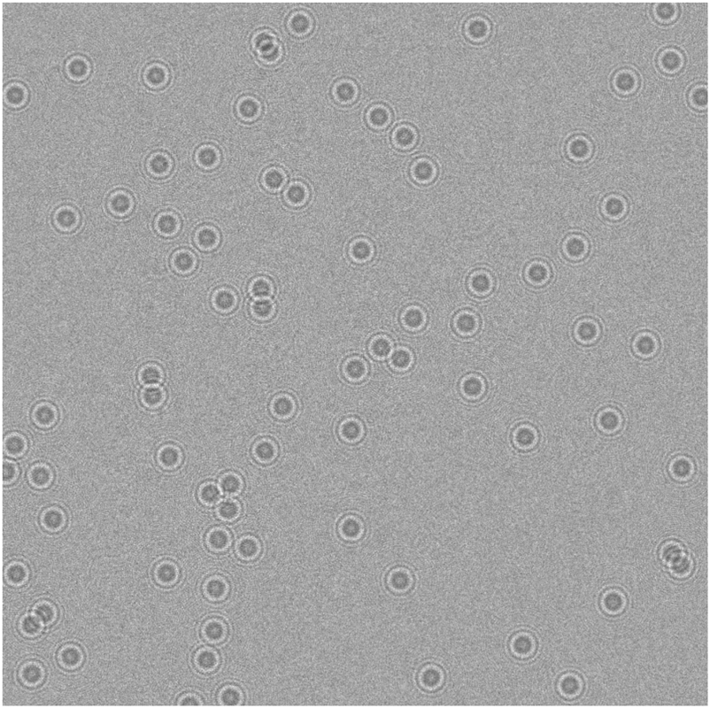
An example of synthetically generated hologram. For visualization purposes, just a piece (800 × 800 pixel) of the frame is shown here. The real frame is larger (800 × 2,184 pixel).
Analysis
We used Python 3.9 to develop an analysis tool that can process the videos acquired by the sensor and estimate the flow rate in the channel. This tool can be broken down into five sequential modules (Figure 7).
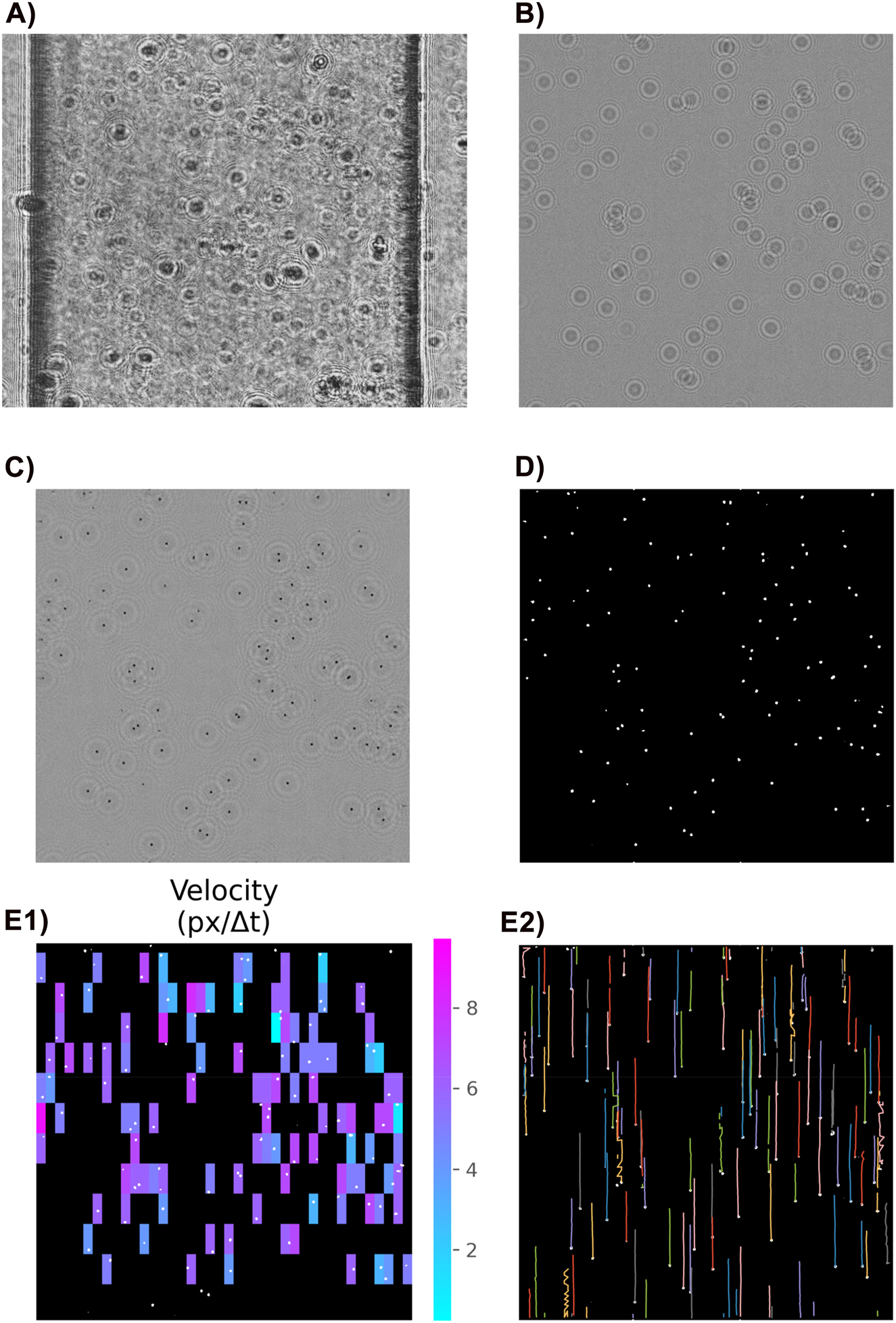
An example of a video frame after being processed by each module of the analysis tool. For visualization purposes, just a piece (800 × 800 pixel) of a frame is shown here. The real frame is larger (800 × 2,184 pixel). The modules are: A) Conversion to gray-scale, B) crop and background subtraction, C) holographic reconstruction, D) particles segmentation, E1) PIV. Due to the particle sparsity, it is not possible to calculate the velocity for all image patches. Those appear black in the image, E2) PTV. Some trajectories contain zigzags. This may happen when two particles move side-by-side very close to each other. In this situation, the algorithm may fail to differentiate them. Fortunately, this has no strong impact on the final flow rate calculation, because it is relatively rare, and it has minimum effect on the velocity aligned with the flow direction, which is the information that is used to calculate the flow rate.
The first module reads the video frames, converts them from RGB to gray-scale, and, if necessary, rotates them so that the flow is in the z-direction.
As shown in Figure 7A, the images are quite cluttered by the channel’s imperfections and impurities attached to the sealing tape. In the second module of the analysis tool, those artifacts are removed by subtracting from the frames an image where no particles are present. This background image is generated by calculating the median between all frames in the video. After the background subtraction, only the moving particles (and a certain level of noise) are visible on the images, as shown in Figure 7B.
After the background subtraction, the interference patterns are sufficiently visible on the frames, and we can proceed with the holographic reconstruction. For the reconstruction, we relied on the Python package Holopy [13]. The result of a reconstruction is an image where each pixel is a vector with magnitude and phase. However, we discarded the phase, because just the magnitude (light intensity) is relevant to the velocimetry methods. For each hologram, we performed six reconstructions with different focal distances. The final image was the pixel-wise minimum of the six reconstructions. This ensures that all the particles, regardless of how far they are from the image sensor, will be depicted as sharp black dots as shown in Figure 7C.
The next module is responsible for segmenting the images that are the result of the holographic reconstruction. Here, segmentation means to generate a binary image where particle pixels have value one, while all the others have value zero, as shown in Figure 7D. For that, we first applied a median filter with a 3 × 3 kernel to minimize speckle noise, then used Yen’s thresholding method [14] to generate the binary image.
Once the frames have been segmented, we can run a particle velocimetry technique (PIV or PTV) to determine the flow rate. PIV (Figure 7E1) operates on the principle that particles that are close together move with similar velocities. Therefore, it divides each frame into many small patches and calculates the cross-correlation of each patch with its corresponding patch in the subsequent frame. The argmax of the cross-correlation provides an estimate of the particle displacement of that specific frame patch. By averaging each of the patch displacements, across all the frames, it is possible to calculate average particle velocity in an image sequence. In a video with n frames, where each frame F is divided into k rows and i columns, the average particle velocity v can be estimated as:
Equation (1):
Where Δt is the time interval in seconds (1/frame rate), and pixel_size is the sensor’s pixel size in µm. S(t, x, z) is the displacement estimated at frame t for the patch located at row z and column x:
Equation (2):
The cross-correlation (represented by the symbol
PTV (Figure 7E2), on the other hand, relies on a very different principle. PTV tries to find the white spots in subsequent frames that represent the same particle. Once this process is done for all frames, we can trace the trajectory of the individual particles. From the length and time stamps of these trajectories, one can calculate the particle velocity. Finally, the average flow velocity v in z-direction can be estimated as the mean particle velocity. Our PTV analysis relies on the package TrackPy [15], which is a Python implementation of the algorithm by Crocker and Grier [16].
For both velocimetry methods, the average flow velocity is calculated as a simple mean of all measured particles (PTV) or patches (PIV) velocities. The simple mean gives a valid estimate because the particles are fairly uniformly distributed in space. Such a distribution has also been observed in other studies working with low Reynolds flows [2, 12].
Finally, the flow rate in nL/min is calculated as:
Equation (3):
Where v is the average flow velocity in µm/s, v sink is the average particle sedimentation velocity in µm/s (in z-direction, since the channel is mounted vertically), and ch_area is the channel area in µm2. We estimated v sink by evaluating Equation (2) for image sequences with no flow (syringe pump turned off). On average, particles sedimented at 15.6 μm/s.
Results
Figure 8 shows the predictions made by our method on the synthetic data. We tested both velocimetry algorithms (PIV and PTV) and observed that they predict very similar values. The average absolute deviation between them is 1.52 nL/min. A difference of only 0.067 pixels when estimating the particles’ displacement from one frame to the next. There is also a good agreement between the reference flow rate set on the simulation and the estimated flow rate. The Mean Relative Error (MRE) for PIV and PTV were 2.2 and 2.6%, respectively. The MRE is defined as shown in Equation (4):
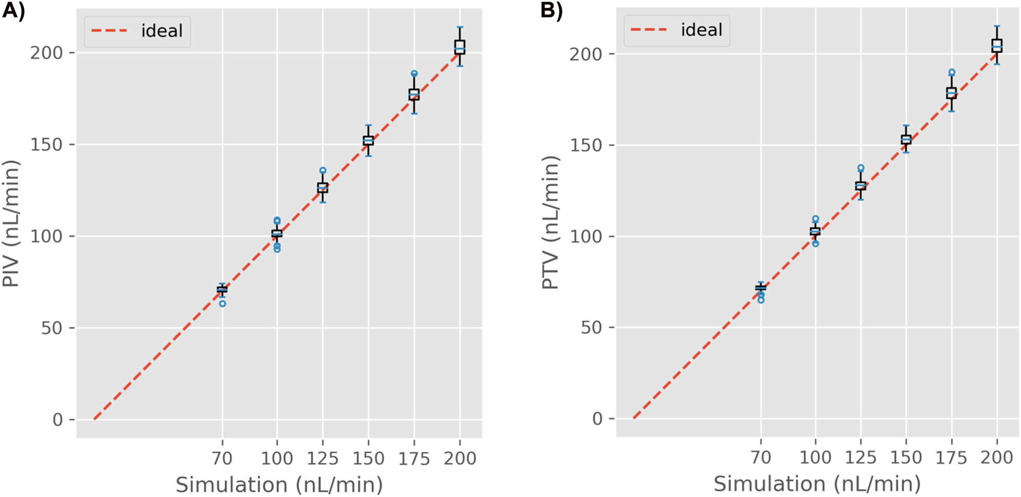
A) Results on the synthetic data using PIV, and B) using PTV shown as standard boxplots.
Equation 4:
where n is the number of times a measurement q i was repeated for a fixed reference q ref (pump setpoint).
Measurement uncertainty
Using the top-down approach described by G. White [17], we calculated out method’s expanded relative uncertainty (U % ):
Equation 5:
where:
k: coverage factor. We adopted k = 2 (95.4% confidence interval).
q m : average measured flow rate.
u c : combined standard uncertainty.
u imp : imprecision due to random effects. It is given by the standard deviation of the measurements (σq).
u bias : uncertainty in the measurement bias.
u ref : uncertainty in the reference flow rate. Since this data was generated by simulation, this uncertainty is very low and was neglected in the calculations (uref = 0).
u rep : uncertainty in the average measurement (q m ) value. Calculated as the standard error of the mean (σ q /√n, where n is the number of measurements).
The uncertainty numbers are shown in detail in Table 1 and summarized in Figure 9. Both velocimetry methods performed similarly well. Their relative uncertainty remained under 6% across the investigated flow rate range. However, PTV performed slightly better. Its uncertainty stayed between 3.9 and 4.9%, while for PIV the values ranged from 4.2 to 5.6%.
Uncertainty components of both velocimetry methods as a function of the reference flow rate.
| qref | PIV | PTV | ||||||||
|---|---|---|---|---|---|---|---|---|---|---|
| (nL/min) | u imp | u rep | u bias | u c | U % (k=2) | u imp | u rep | u bias | u c | U % (k=2) |
| 70 | 1.8975 | 0.1897 | 0.1897 | 1.9069 | 5.40 | 1.6463 | 0.1646 | 0.1646 | 1.6545 | 4.63 |
| 100 | 2.7966 | 0.2797 | 0.2797 | 2.8105 | 5.56 | 2.5216 | 0.2522 | 0.2522 | 2.5342 | 4.94 |
| 125 | 3.3205 | 0.3320 | 0.3320 | 3.3370 | 5.28 | 3.0382 | 0.3038 | 0.3038 | 3.0533 | 4.78 |
| 150 | 3.1987 | 0.3199 | 0.3199 | 3.2146 | 4.24 | 2.9463 | 0.2946 | 0.2946 | 2.9610 | 3.87 |
| 175 | 4.3310 | 0.4331 | 0.4331 | 4.3526 | 4.92 | 3.9938 | 0.3994 | 0.3994 | 4.0137 | 4.50 |
| 200 | 4.9916 | 0.4992 | 0.4992 | 5.0165 | 4.95 | 4.7824 | 0.4782 | 0.4782 | 4.8062 | 4.71 |
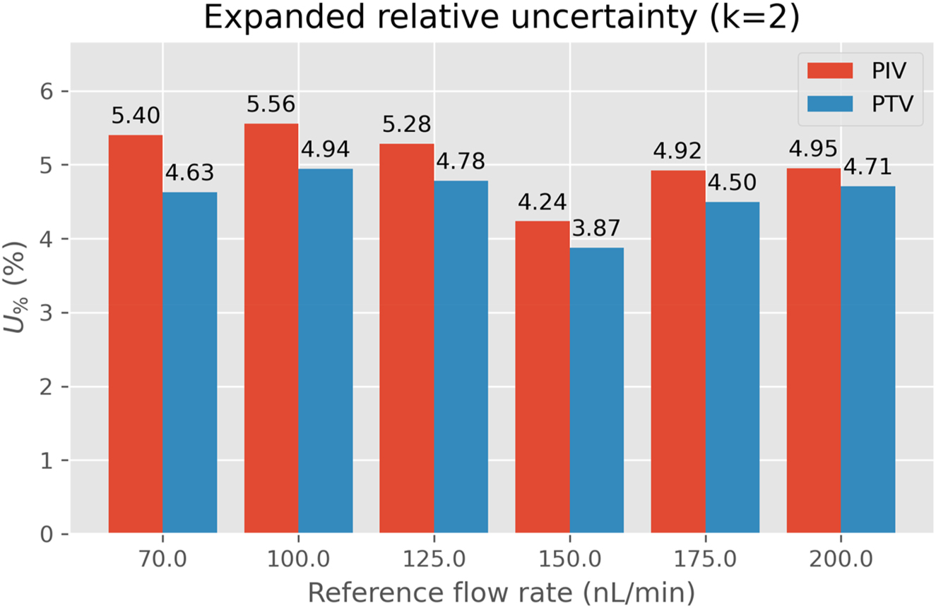
Expanded relative uncertainty for a coverage factor of 2.
Experimental data
Comparing the predictions of the velocimetry methods on the experimental data (Figure 10) one can see that the predictions of both methods only differ by a few fractions of a pixel; 0.082 pixel/Δt on average. Such a “cross-validation” between the methods is indicative that the velocimetry modules are functioning as required.
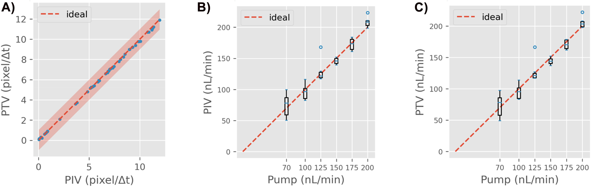
Results on the experimental data. A) PTV vs PIV estimates. Each blue dot corresponds to one of the 50 measurements in the dataset. The red-shaded region marks where the deviation is less than one pixel/Δt. The two methods predict very similar values. The deviation is always in the sub-pixel range. B) Flow rates obtained with PIV vs. syringe pump setpoint. C) Flow rates obtained with PTV vs. syringe pump setpoint. Figures B and C use standard boxplots.
Figure 10B and C compare the estimated flow rate with the setpoint used by the syringe pump. We observe a good average agreement between these quantities; the MRE was 9.1% for PIV, and 8.8% for PTV. Still, two outliers are present and the errors for the lowest reference flow rate (70 nL/min) were considerably higher. Possible causes of these errors are presented in the next section.
Discussion
It was demonstrated that a combination of LDHM with particle velocimetry can be used to reliably measure flow rates in the nL/min range. Using synthetic data, we obtained an MRE of less than 3%. On the other hand, the error was considerably higher on the experimental data, around 9%. This higher error was identified as instabilities in the flow rate during the measurements. For instance, the data point with the largest error we encountered was measured as 168.8 nL/min whereas its reference was 125 nL/min; resulting in an error of 35%. When plotting the instantaneous (i.e. frame-by-frame) flow rate estimate for this data point (Figure 11A), we observe that it was not stable during the measurement. Its value decreased 40 nL/min almost linearly between the first and last frame. To verify if this effect is present in the other data points, we calculate coefficient of variation (CV = standard deviation/mean) among the instantaneous flow rates for each video. The CV among the instantaneous flow rates can be used as an estimate of the flow rate stability of a single video. Figure 11B shows that there is a correlation between the CV and the error, indicating that the error is larger for videos with unstable flow rates. Moreover, Figure 11C shows what MRE (y-axis) would be obtained if we excluded videos with a CV higher than a certain cutoff (x-axis). We see that, the lower the cutoff, the lower the MRE, which reinforces the conclusion that the videos where the flow rate was not stable were those with high errors. For a CV cutoff of 2%, the MRE is less than 4%, which is similar to what was obtained on the synthetic data.
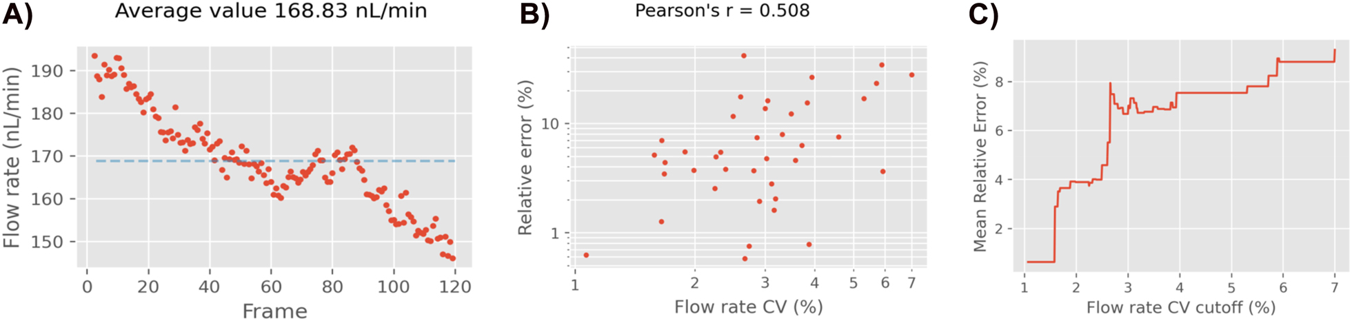
The effects of the instantaneous flow rate stability. A) The instantaneous flow rate of the measurement with the largest error. The expected value was 125 nL/min, however the flow was not settled at the moment of the measurement. B) Scatter plot of the relative error vs. the instantaneous flow rate stability (CV). More stable flow rates tend to have lower measurement errors. C) The effects of cleaning the dataset with a flow rate CV cutoff. The lower the cutoff, the lower is the MRE.
One source of instability may have been the pumping system itself. According to its datasheet, the syringe pump operates in pulsation mode for flow rates under 1,042 nL/min. The pulsation mode not only fails to provide a constant instantaneous flow rate but also has reduced dosing precision [18]. This hypothesis gains strength when we consider that, for the experimental data, the errors were significantly higher for the lowest reference flow rate (70 nL/min), where the pulsation effects become more pronounced. This error increase was not observed in the synthetic data, therefore, it cannot be attributed to limitations in data resolution or analysis method. Other possible sources of instability may have been mechanical perturbations during the measurements, fluidic capacitance (due to tubing elasticity), air bubbles, or leaks in the tubing connections.
It is also shown that our method achieves subpixel accuracy. While the precision in measuring the particles’ position is related to the sensor’s pixel size, the mutual agreement of the velocimetry methods (Figure 10A) and the results on the synthetic data (Figure 8) show that the precision in estimating the particle’s velocity is not constrained to 1 pixel/Δt. In the case of PIV, this is a consequence of averaging the population of patch displacement estimates (Equation (1)). A single patch displacement estimate (Equation (2)) is a discrete number given in pixels, but when a population of those estimates is averaged, the answer converges to the actual displacement value in the continuous space. In our experiments, the flow rate of each video is obtained by averaging approximately 11,500 patch estimates. In the case of PTV, the same mechanism applies. Approximately 230 particles were present in each frame, meaning that the final velocity is an average of 27,600 (230 particles × 120 frames) individual velocity estimates. Additionally, the PTV algorithm (as implemented by TrackPy) calculates the centroid of each particle, which results in a continuous value. Interestingly, our PIV implementation does not contain any of such an a-priory sub-pixel refinement and still manages to obtain sub-pixel accuracy. This is evidence that averaging alone can deliver sub-pixel accuracy given that the averaged population is large enough.
Our holographic reconstruction was two-dimensional. All particles, regardless of their depth in the channel, are displayed in a single image. As a consequence, the reconstructed sequence of images will display particles moving at very different speeds, even those that are close together. While this does not affect the operation of PTV, it does violate the most basic assumption of PIV: particles in the same neighborhood, move at similar velocities. Still, PIV manages to provide good results. Such an unexpected outcome can be explained by two reasons. First, the particles are sparsely distributed, which means that most of the patches contain a single particle (Figure 7E1), and, therefore, no violation of the PIV’s assumption occurs. Second, even if the particles were densely distributed, the final flow rate estimate is the product of averaging thousands of patch velocities. The regression toward the mean effect makes the final estimate converge to the correct value. Still, a three-dimensional holographic reconstruction may be beneficial to the overall precision of PIV, also accelerating its convergence. The price to pay is a more complicated reconstruction process, which increases the software runtime.
The precision obtained with PIV and PTV was quite similar. However, PIV required a higher level of algorithm refinement, while the PTV package utilized (TrackPy) met our requirements without much tuning. In first attempts, the PIV algorithm was implemented in its traditional 2D formulation. The results were not satisfactory because many of the velocity vectors were calculated based on spurious particle correlations. To overcome this issue, an increase in particle density would be required, but that would be detrimental to the holography reconstruction. The solution adopted instead was to use a 1D PIV formulation, which requires fewer particles since it assumes that the flow direction is unique and known in the entirety of the channel. Regarding the runtime of each algorithm, PIV was on average 25% faster than PTV.
Conclusions
In this paper, a method combining LDHM and particle velocimetry to measure low flow rates in the nL/min range has been demonstrated. An experimental setup has been established, where particles were pumped though a custom made channel via a syringe pump while an image sequence was recorded with a LDHM setup. An analysis tool was developed to reconstruct the holograms and analyze them using different particle velocimetry methods. Using large amounts of simulated data, the analysis tool was validated and the uncertainty of the method was estimated. The CAD designs and source-codes were made freely available for download.
As expected, a larger error occurred in the experimental measurements which in future trials could be minimized by conducting the experiment in a quieter environment while using a syringe with a smaller diameter. This would result in a pulsation-free pumping system increasing its dosing precision. It was also shown that both particle imaging velocimetry (PIV) and particle tracing velocimetry (PTV) are suitable methods to measure such low flow rates and only differ substantially in their runtime. Future work will extend the investigations into even lower flow ranges (bellow 70 nL/min), which has not been done in this article due to the limits of the syringe pump. Another aspect that may also be improved is the reconstruction of the holograms as three-dimensional volumes instead of in a single two-dimensional image. This may reduce the PIV errors and will provide an estimate of the three-dimensional flow profile.
Funding source: European Association of National Metrology Institutes
Award Identifier / Grant number: 18 HLT08 MeDDII (EMPIR)
-
Research funding: This work performed under 18 HLT08 MeDDII project has received funding from the EMPIR programme co-financed by the Participating States and from the European Union’s Horizon 2020 research and innovation programme.
-
Author contributions: All authors have accepted responsibility for the entire content of this manuscript and approved its submission.
-
Competing interests: Authors state no conflict of interest.
-
Informed consent: Informed consent was obtained from all individuals included in this study.
-
Ethical approval: The local Institutional Review Board deemed the study exempt from review.
References
1. Snijder, RA, Konings, MK, Lucas, PT, Egberts, C, Timmerman, AD. Flow variability and its physical causes in infusion technology: a systematic review of in vitro measurement and modeling studies. Biomed Eng Tech 2015;60:277–300. https://doi.org/10.1515/bmt-2014-0148.Search in Google Scholar PubMed
2. Kim, S, Lee, SJ. Measurement of 3D laminar flow inside a micro tube using micro digital holographic particle tracking velocimetry. J Micromech Microeng 2007;17:2157–62. https://doi.org/10.1088/0960-1317/17/10/030.Search in Google Scholar
3. Salipante, P, Hudson, SD, Schmidt, JW, Wright, JD. Microparticle tracking velocimetry as a tool for microfluidic flow measurements. Exp Fluid 2017;58:85. https://doi.org/10.1007/s00348-017-2362-6.Search in Google Scholar
4. Melling, A. Tracer particles and seeding for particle image velocimetry. Meas Sci Technol 1997;8:1406. https://doi.org/10.1088/0957-0233/8/12/005.Search in Google Scholar
5. Gharib, M, Willert, C. Particle tracing: revisited. In: Advances in fluid mechanics measurements. Springer; 1989:109–26 pp.10.1007/978-3-642-83787-6_3Search in Google Scholar
6. Scharnowski, S, Kähler, CJ. Particle image velocimetry - classical operating rules from today’s perspective. Opt Laser Eng 2020;135:106185. https://doi.org/10.1016/j.optlaseng.2020.106185.Search in Google Scholar
7. Garcia-Sucerquia, J, Xu, W, Jericho, SK, Klages, P, Jericho, MH, Kreuzer, HJ. Digital in-line holographic microscopy. Appl Opt 2006;45:836–50. https://doi.org/10.1364/ao.45.000836.Search in Google Scholar PubMed
8. Gabor, D. A new microscopic principle. Nature 1948;161:777–8. https://doi.org/10.1038/161777a0.Search in Google Scholar PubMed
9. Ozcan, A, McLeod, E. Lensless imaging and sensing. Annu Rev Biomed Eng 2016;18:77–102. https://doi.org/10.1146/annurev-bioeng-092515-010849.Search in Google Scholar PubMed
10. Deng, Y, Chu, D. Coherence properties of different light sources and their effect on the image sharpness and speckle of holographic displays. Sci Rep 2017;7:1–12. https://doi.org/10.1038/s41598-017-06215-x.Search in Google Scholar PubMed PubMed Central
11. The OpenFOAM Foundation. icoFoam [Internet]; 2019. Available from: www.openfoam.org.Search in Google Scholar
12. Sommer, C, Quint, S, Spang, P, Walther, T, Baßler, M. Studying the Segré-Silberberg effect by velocimetry in microfluidic channels, Coruña, A, editor. Spain; 2014:265–77 pp. Available from: http://library.witpress.com/viewpaper.asp?pcode=AFM14-023-1 [Accessed 10 Oct 2022].10.2495/AFM140231Search in Google Scholar
13. Barkley, S, Dimiduk, TG, FungKaz, JDM, Manoharan, VN, McGorty, R, Perry, RW, Wang, A. Holographic microscopy with Python and HoloPy. Comput Sci Eng 2019;22:72–82.10.1109/MCSE.2019.2923974Search in Google Scholar
14. Yen, JC, Chang, FJ, Chang, S. A new criterion for automatic multilevel thresholding. IEEE Trans Image Process 1995;4:370–8. https://doi.org/10.1109/83.366472.Search in Google Scholar PubMed
15. Allan, DB, Caswell, T, Keim, NC, van der Wel, CM, Verweij, RW. Soft-matter/trackpy: Trackpy v0.5.0. Geneva, Switzerland: Zenodo; 2021.Search in Google Scholar
16. Crocker, JC, Grier, DG. Methods of digital video microscopy for colloidal studies. J Colloid Interface Sci 1996;179:298–310. https://doi.org/10.1006/jcis.1996.0217.Search in Google Scholar
17. White, GH. Basics of estimating measurement uncertainty. Clin Biochem Rev 2008;29:S53.Search in Google Scholar
18. Cetoni GmbH. neMESYS low pressure – hardware manual and reference; 2020. Report No.: 1.01. Available from: www.cetoni.de.Search in Google Scholar
© 2022 the author(s), published by De Gruyter, Berlin/Boston
This work is licensed under the Creative Commons Attribution 4.0 International License.
Articles in the same Issue
- Frontmatter
- Guest Editorial
- Medical flow and dosing measurement metrology in drug delivery
- Special Issue Articles
- Metrology in health: challenges and solutions in infusion therapy and diagnostics
- Calibration methods for flow rates down to 5 nL/min and validation methodology
- Measurement of internal diameters of capillaries and glass syringes using gravimetric and optical methods for microflow applications
- In-line measurements of the physical and thermodynamic properties of single and multicomponent liquids
- Assessment of drug delivery devices working at microflow rates
- Calibration of insulin pumps based on discrete doses at given cycle times
- Development of a microfluidic electroosmosis pump on a chip for steady and continuous fluid delivery
- Effect of non-return valves on the time-of-arrival of new medication in a patient after syringe exchange in an infusion set-up
- Holographic PIV/PTV for nano flow rates–A study in the 70 to 200 nL/min range
- Unexpected dosing errors due to air bubbles in infusion lines with and without air filters