Startseite Mathematik Hierarchy structures in finite index CMC surfaces
Artikel Open Access

Hierarchy structures in finite index CMC surfaces

  • William H. Meeks III und Joaquín Pérez ORCID logo EMAIL logo
Veröffentlicht/Copyright: 26. Juli 2023

Abstract

Given ε 0 > 0 , I { 0 } and K 0 , H 0 0 , let X be a complete Riemannian 3-manifold with injectivity radius Inj ( X ) ε 0 and with the supremum of absolute sectional curvature at most K 0 , and let M X be a complete immersed surface of constant mean curvature H [ 0 , H 0 ] with index at most I. For such M X , we prove a structure theorem which describes how the interesting ambient geometry of the immersion is organized locally around at most I points of M, where the norm of the second fundamental form takes on large local maximum values.

MSC 2020: 53A10; 49Q05; 53C42

1 Introduction

Let X denote a complete Riemannian 3-manifold with positive injectivity radius Inj ( X ) and bounded absolute sectional curvature. Let M be a complete immersed surface in X of constant mean curvature H 0 ; we call M an H-surface in X. The Jacobi operator of M is the Schrödinger operator

L = Δ + | A M | 2 + Ric ( N ) ,

where Δ is the Laplace–Beltrami operator on M, | A M | 2 is the square of the norm of its second fundamental form, and Ric ( N ) denotes the Ricci curvature of X in the direction of the unit normal vector N to M; the index of M is the index of L:

Index ( M ) = lim R Index ( B M ( p , R ) ) ,

where B M ( p , R ) is the intrinsic metric ball in M of radius R > 0 centered at a point p M , and Index ( B M ( p , R ) ) is the number of negative eigenvalues of L on B M ( p , R ) with Dirichlet boundary conditions. Here, we have assumed that the immersion is two-sided (this holds in particular if H > 0 ). In the case that H = 0 and the immersion is one-sided, the index is defined in a similar manner using compactly supported variations in the normal bundle; see Definition 2.1 for details.

The primary goal of this paper is to describe the structure of complete immersed H-surfaces F : M X (also called H-immersions) which have a fixed bound I { 0 } on their index and a fixed upper bound H 0 for their constant mean curvatures H, in certain small intrinsic neighborhoods of points with sufficiently large norm | A M | of their second fundamental forms; see Theorem 1.2. When M has non-empty boundary, we will assume, after a choice of some ε 0 ( 0 , Inj ( X ) ) , that there is an upper bound A 0 of | A M | in the intrinsic ε 0 -neighborhood of the boundary of M. Theorem 1.2 plays an important theoretical role in understanding global properties of such surfaces in much the same way that the local structure theorems of Colding and Minicozzi [7, 8] (for embedded minimal surfaces) and of Meeks and Tinaglia [21] (for embedded H-surfaces with H > 0 ) play a fundamental role in understanding global properties of complete embedded H-surfaces of finite genus, especially in the case where X = 3 . However, we point out that the results in this paper do not depend on the results for embedded H-surfaces of Colding–Minicozzi and Meeks–Tinaglia; for applications of Theorem 1.2 to the global theory of finite index H-surfaces in Riemannian 3-manifolds, see [18].

In the sequel, we will denote by B X ( x , r ) (resp. B ¯ X ( x , r ) ) the open (resp. closed) metric ball centered at a point x X of radius r > 0 . For a Riemannian surface M with smooth compact boundary M , κ ( M ) = M κ g will stand for the total geodesic curvature of M , where κ g denotes the pointwise geodesic curvature of M with respect to the inward pointing unit conormal vector of M along M .

Definition 1.1.

For every I { 0 } , ε 0 > 0 and H 0 , A 0 , K 0 0 , we denote by

Λ = Λ ( I , H 0 , ε 0 , A 0 , K 0 )

the space of all H-immersions F : M X satisfying the following conditions:

  1. X is a complete Riemannian 3-manifold with injectivity radius Inj ( X ) ε 0 and absolute sectional curvature bounded from above by K 0 .

  2. M is a complete surface with smooth boundary (possibly empty), and when M , there are points in M of distance greater than ε 0 from M .

  3. H [ 0 , H 0 ] and F has index at most I.

  4. If M , then for any ε ( 0 , ] we let

    U ( M , ε ) = { x M d M ( x , M ) < ε }

    be the open intrinsic ε -neighborhood of M . Then | A M | is bounded from above by A 0 in U ( M , ε 0 ) .

Suppose that ( F : M X ) Λ and M . For any positive ε 1 ε 2 [ 0 , ] , let

U ( M , ε 1 , ε 2 ) = U ( M , ε 2 ) U ( M , ε 1 ) ¯ , U ¯ ( M , ε 1 , ε 2 ) = U ( M , ε 2 ) ¯ U ( M , ε 1 ) .

When M = , we define U ( M , ε 1 , ) = U ¯ ( M , ε 1 , ) as M.

In the next result, we will make use of harmonic coordinates φ x : U B X ( x , r ) defined on an open subset U of 3 containing the origin, taking values in a geodesic ball B X ( x , r ) centered at a point x X of positive radius r less than the injectivity radius of X at x and with a C 1 , α control of the ambient metric on X; see Definition 2.2 for details.

Theorem 1.2 (Structure Theorem for finite index H-surfaces).

Suppose that ε 0 > 0 , K 0 , H 0 , A 0 0 , I N { 0 } , and τ ( 0 , π / 10 ] are given. Then there exist A 1 [ A 0 , ) and δ 1 , δ ( 0 , ε 0 / 2 ] , with δ 1 δ / 2 , such that, for any

( F : M X ) Λ = Λ ( I , H 0 , ε 0 , A 0 , K 0 ) ,

there exists a (possibly empty) finite collection

𝒫 F = { p 1 , , p k } U ( M , ε 0 , )

of points, k I , and numbers r F ( 1 ) , , r F ( k ) [ δ 1 , δ 2 ] with r F ( 1 ) > 4 r F ( 2 ) > > 4 k - 1 r F ( k ) , satisfying the following properties:

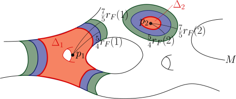
  1. Portions with concentrated curvature: Given i = 1 , , k , let Δ i be the component of F - 1 ( B ¯ X ( F ( p i ) , r F ( i ) ) ) containing p i . Then the following assertions hold:

    1. Δ i B ¯ M ( p i , 5 4 r F ( i ) ) (in particular, Δ i is compact).

    2. Δ i has smooth boundary and F ( Δ i ) B ¯ X ( F ( p i ) , r F ( i ) ) .

    3. For i j ,

      B M ( p i , 7 5 r F ( i ) ) B M ( p j , 7 5 r F ( j ) ) = .

      In particular, the intrinsic distance between Δ i and Δ j is greater than 3 10 δ 1 for every i j .

    4. It holds

      | A M | ( p i ) = max Δ i | A M | = max { | A M | ( p ) | p M j = 1 i - 1 B M ( p j , 5 4 r F ( j ) ) } A 1 ;

      see Figure 1.

    5. The index Index ( Δ i ) of Δ i is positive.

  2. Transition annuli: For i = 1 , , k fixed, let e ( i ) be the number of boundary components of Δ i . Then there exist planar disks 𝔻 1 , , 𝔻 e ( i ) T F ( p i ) X of radius 2 r F ( i ) centered at the origin in T F ( p i ) X such that, if we set

    P i , h = φ F ( p i ) ( 𝔻 h ) , h { 1 , , e ( i ) } ,

    where φ F ( p i ) denotes a harmonic chart centered at F ( p i ) , see Definition 2.2 , then

    F ( Δ i ) [ B ¯ X ( F ( p i ) , r F ( i ) ) B X ( F ( p i ) , r F ( i ) 2 ) ]

    consists of e ( i ) annular multi-graphs [1] G i , 1 , , G i , e ( i ) over their projections to P i , 1 , , P i , e ( i ) , with multiplicities m i , 1 , , m i , e ( i ) , respectively, and whose related graphing function u satisfies

    (1.1) | u ( x ) | | x | + | u | ( x ) τ ,

    where we have taken coordinates x in each of the P i , h and denoted by | x | the extrinsic distance to F ( p i ) in the ambient metric of X ; see Figure 2.

  3. Region with uniformly bounded curvature: | A M | < A 1 on M ~ := M i = i k Int ( Δ i ) .

Moreover, the following additional properties hold:

  1. i = 1 k I ( Δ i ) I , where I ( Δ i ) = Index ( Δ i ) .

  2. Geometric and topological estimates: Given i = 1 , , k , let m ( i ) := h = 1 e ( i ) m i , h be the total spinning of the boundary of Δ i , let g ( Δ i ) denote the genus of Δ i (in the case that Δ i is non-orientable, g ( Δ i ) denotes the genus of its oriented cover [2] ). Then m ( i ) 2 and the following upper estimates hold:

    1. If I ( Δ i ) = 1 , then Δ i is orientable, g ( Δ i ) = 0 and ( e ( i ) , m ( i ) ) { ( 2 , 2 ) , ( 1 , 3 ) } .

    2. If Δ i is orientable and I ( Δ i ) 2 , then m ( i ) 3 I ( Δ i ) - 1 , e ( i ) 3 I ( Δ i ) - 2 and g ( Δ i ) 3 I ( Δ i ) - 4 .

    3. If Δ i is non-orientable, then I ( Δ i ) 2 , m ( i ) 3 I ( Δ i ) - 1 , e ( i ) 3 I ( Δ i ) - 2 , and g ( Δ i ) 6 I ( Δ i ) - 8 .

    4. χ ( Δ i ) - 6 I ( Δ i ) + 2 m ( i ) + e ( i ) , and thus

      χ ( i = 1 k Δ i ) - 6 I + 2 S + e ,

      where

      e = i = 1 k e ( i ) , S = i = 1 k m ( i ) .

    5. | κ ( Δ i ) - 2 π m ( i ) | τ m ( i ) , and so the total geodesic curvature κ ( M ~ ) of M ~ along M ~ M satisfies

      | κ ( M ~ ) + 2 π S | τ 2 k ,

      and so

      (1.2) 2 π S - τ 2 k i = 1 k κ ( Δ i ) 2 π S + τ 2 k .

    6. - Δ i K > 3 π , and so

      (1.3) - i = 1 k Δ i K = - 2 π χ ( i = 1 k Δ i ) + i = 1 k Δ i κ g > 3 k π .

  3. Genus estimate outside the concentration of curvature: If M is orientable, k 1 and the genus g ( M ) of M is finite, then the genus g ( M ~ ) of M ~ satisfies

    0 g ( M ) - g ( M ~ ) 3 I - 2 .

  4. Area estimate outside the concentration of curvature: If k 1 , then

    Area ( M ~ ) 14 π i = 1 k m ( i ) r F ( i ) 2 2 π i = 1 k m ( i ) r F ( i ) 2 Area ( i = 1 k Δ i ) k π δ 1 2 .

  5. There exists a C > 0 , depending on ε 0 , K 0 , H 0 and independent of I , such that

    (1.4) Area ( M ) { C max { 1 , Radius ( M ) } if  M , C max { 1 , Diameter ( M ) } if  M = ,

    where

    Radius ( M ) = sup x M d M ( x , M ) ( 0 , ] if  M ,
    Diameter ( M ) = sup x , y M d M ( x , y ) if  M = .

    In particular, if M has infinite radius or if M has empty boundary and it is non-compact, then its area is infinite.

Figure 1 
               The second fundamental form concentrates
inside the intrinsic compact regions 


                              Δ
                              i


                        {\Delta_{i}}
                     
                   (in red),
each of which is mapped through the immersion F
to a surface inside the extrinsic ball in X centered at


                              F
                              ⁢
                              
                                 (
                                 
                                    p
                                    i
                                 
                                 )


                        {F(p_{i})}
                     
                   of radius 


                                    r
                                    F
                                 
                                 ⁢
                                 
                                    (
                                    i
                                    )
                                 
                              
                              >
                              0


                        {r_{F}(i)>0}
                     
                  , with 


                                 F
                                 ⁢
                                 
                                    (
                                    
                                       ∂
                                       ⁡
                                       
                                          Δ
                                          i
                                       
                                    
                                    )
                                 
                              
                              ⊂
                              
                                 
                                    ∂
                                    ⁡
                                    
                                       
                                          B
                                          ¯
                                       
                                       X
                                    
                                 
                                 ⁢
                                 
                                    (
                                    
                                       F
                                       ⁢
                                       
                                          (
                                          
                                             p
                                             i
                                          
                                          )
                                       
                                    
                                    ,
                                    
                                       
                                          r
                                          F
                                       
                                       ⁢
                                       
                                          (
                                          i
                                          )
                                       
                                    
                                    )


                        {F(\partial\Delta_{i})\subset\partial\overline{B}_{X}(F(p_{i}),r_{F}(i))}
                     
                  .
Although the boundary 


                              ∂
                              ⁡
                              
                                 Δ
                                 i


                        {\partial\Delta_{i}}
                     
                   might not be at constant
intrinsic distance from the ‘center’ 


                              p
                              i


                        {p_{i}}
                     
                  , 


                              Δ
                              i


                        {\Delta_{i}}
                     
                   lies entirely
inside the intrinsic ball centered at 


                              p
                              i


                        {p_{i}}
                     
                  of radius 


                                 5
                                 4
                              
                              ⁢
                              
                                 r
                                 F
                              
                              ⁢
                              
                                 (
                                 i
                                 )


                        {\frac{5}{4}r_{F}(i)}
                     
                  .
The intrinsic open balls 


                                 B
                                 M
                              
                              ⁢
                              
                                 (
                                 
                                    p
                                    i
                                 
                                 ,
                                 
                                    
                                       7
                                       5
                                    
                                    ⁢
                                    
                                       r
                                       F
                                    
                                    ⁢
                                    
                                       (
                                       i
                                       )
                                    
                                 
                                 )


                        {B_{M}(p_{i},\frac{7}{5}r_{F}(i))}
                     
                   are pairwise disjoint.
Figure 1

The second fundamental form concentrates inside the intrinsic compact regions Δ i (in red), each of which is mapped through the immersion F to a surface inside the extrinsic ball in X centered at F ( p i ) of radius r F ( i ) > 0 , with F ( Δ i ) B ¯ X ( F ( p i ) , r F ( i ) ) . Although the boundary Δ i might not be at constant intrinsic distance from the ‘center’ p i , Δ i lies entirely inside the intrinsic ball centered at p i of radius 5 4 r F ( i ) . The intrinsic open balls B M ( p i , 7 5 r F ( i ) ) are pairwise disjoint.

Figure 2 
               The transition annuli: On the right, one has the extrinsic
representation in X of one of the annular multi-graphs G in


                                 F
                                 ⁢
                                 
                                    (
                                    
                                       Δ
                                       1
                                    
                                    )
                                 
                              
                              ∩
                              
                                 [


                                             B
                                             ¯
                                          
                                          X
                                       
                                       ⁢
                                       
                                          (
                                          
                                             F
                                             ⁢
                                             
                                                (
                                                
                                                   p
                                                   1
                                                
                                                )
                                             
                                          
                                          ,
                                          
                                             
                                                r
                                                F
                                             
                                             ⁢
                                             
                                                (
                                                1
                                                )
                                             
                                          
                                          )
                                       
                                    
                                    ∖
                                    
                                       
                                          B
                                          X
                                       
                                       ⁢
                                       
                                          (
                                          
                                             F
                                             ⁢
                                             
                                                (
                                                
                                                   p
                                                   1
                                                
                                                )
                                             
                                          
                                          ,


                                                   r
                                                   F
                                                
                                                ⁢
                                                
                                                   (
                                                   1
                                                   )
                                                
                                             
                                             /
                                             2
                                          
                                          )


                                 ]


                        {F(\Delta_{1})\cap[\overline{B}_{X}(F(p_{1}),r_{F}(1))\setminus B_{X}(F(p_{1})%
,r_{F}(1)/2)]}
                     
                  ;
in this case, the multiplicity of the multi-graph is 3.
On the left, one has the intrinsic representation of
the same annulus (shadowed); there is one such annular multi-graph for
each boundary component of 


                              Δ
                              i


                        {\Delta_{i}}
                     
                  .
Figure 2

The transition annuli: On the right, one has the extrinsic representation in X of one of the annular multi-graphs G in F ( Δ 1 ) [ B ¯ X ( F ( p 1 ) , r F ( 1 ) ) B X ( F ( p 1 ) , r F ( 1 ) / 2 ) ] ; in this case, the multiplicity of the multi-graph is 3. On the left, one has the intrinsic representation of the same annulus (shadowed); there is one such annular multi-graph for each boundary component of Δ i .

The proof of the Structure Theorem 1.2 is carried out in Section 5, and it will be done by induction on the index bound I. In the case I = 0 , Theorem 1.2 is obtained by using curvature estimates for stable H-surfaces, and the arguments in this special case generalize to the case where, for a given I , there exists a uniform curvature estimate for the immersions in Λ = Λ ( I , H 0 , ε 0 , A 0 , K 0 ) ; see Section 5.1. A non-trivial step in the proof of Theorem 1.2 involves an analysis of the local pictures on different scales for a sequence of complete H n -immersions F n : M n X n with H n [ 0 , H 0 ] and Index ( F n ) I , such that { sup | A M n | } n is unbounded (these local pictures are limits of the F n after blowing up on certain scales). Although non-trivial, this analysis is simpler in the case I = 1 because in this case there is only one scale for the local pictures of F n ; this case is studied in Section 5.4. The analysis of these local pictures in the general case is carried out in Section 5.5, and it is based on the lower bounds obtained by Chodosh and Maximo [6] and Karpukhin [13] for the index of a possibly branched, complete immersed minimal surface Σ in 3 with finite total curvature, in terms of its genus, total branching order, and the number of its ends counted with multiplicity. After coming back to the original scale, these complexity estimates will give upper bounds for the total geodesic curvature of the boundary of the portion M ~ of M defined in Theorem 1.2(iii), as well as to give lower bounds in III on the genus of M ~ in terms of I and the genus of M when M is orientable. These geometric and topological bounds are obtained in Sections 5.6 and 5.7. What this analysis demonstrates is that there is an organized hierarchy-type structure in the geometry of a complete, immersed H-surface F : M X near points of large, almost-maximal norm of the second fundamental form of the immersion, from which the title of the paper is derived; this hierarchy structure of F around such special points is described explicitly in Section 5.6 and plays an essential role in the proofs of our main results.

A key step in the proof of Theorem 1.2 is to obtain curvature estimates for a large portion of the H-surface ( F : M X ) Λ in that theorem. These curvature estimates are obtained in Section 5.2 and they are based on related curvature estimates for stable H-surfaces developed in Section A.

Observe that (1.4) is a lower bound for the area of an H-surface in a Riemannian 3-manifold X, described in terms of an upper bound for its absolute mean curvature function | H | , a lower bound of the injectivity radius of X and an upper bound of the sectional curvature of X. This area estimate is proven in Section 5.7 and follows from a more general area estimate and an intrinsic monotonicity of volume formula for n-dimensional submanifolds with bounded length of their mean curvature vectors in m-dimensional Riemannian manifolds X that have a lower bound for their injectivity radius and an upper bound for the sectional curvature of X. Both of these auxiliary results are proven in our paper [17], and we include their statements (without proofs) in this paper for the sake of completeness; see Propositions B.1 and B.3. In Proposition B.4, we state explicit scale invariant weak chord-arc estimates for finitely branched minimal surfaces of finite total curvature in 3 in terms of the index and total branching (also proven in [17]); these chord-arc estimates are applied in the proof of Theorem 1.2(i).

An important theoretical consequence of the Structure Theorem 1.2 is the existence of compactness results for H-surfaces of bounded index in X. More specifically, in Section 6 we state and prove some compactness results for sequences of complete immersions with constant mean curvature in Λ = Λ ( I , H 0 , ε 0 , A 0 , K 0 ) , as described in Theorem 1.2, in the particular case that the immersions are defined on connected surfaces without boundary, the ambient space X is independent of the element in the sequence, and the image of each immersion in the sequence intersects a fixed compact subdomain of X. In this case, the limit object that we encounter (after passing to a subsequence) is a complete, possibly finitely branched immersion of constant mean curvature at most H 0 and index at most I.

In regards to the just mentioned compactness results in Section 6, it is worth mentioning the related paper [3] by Bourni, Sharp and Tinaglia, where they give weak compactness results for a sequence of embedded CMC hypersurfaces in a compact Riemannian manifold of dimension m with 3 m 7 , provided that their areas and Morse indices are bounded. As they remark in [3], their results were motivated by the derivation of the genus-dependent area bounds for triply periodic CMC surfaces properly embedded in 3 by Meeks and Tinaglia in [22]; also the results in [3] and in our present paper are motivated by other recent works [1, 2, 4, 5, 15, 26], which together help to describe the geometry of finite index CMC surfaces M embedded in closed Riemannian 3-manifolds and relationships between index, area and genus of such an M.

In [18], we give applications of Theorem 1.2 to understand global properties of immersed H-surfaces M X of fixed finite index I, especially results related to the area and diameter of such an M when it is compact without boundary; in particular, we deduce that the area of such an M (resp. the diameter) grows at least linearly (resp. logarithmically) with the genus.

2 Index of one-sided H-immersions, harmonic coordinates and multi-valued graphs

In Theorem 1.2, we referred to the index of one-sided minimal immersions, harmonic coordinates and finitely valued multi-graphs. We will devote this section to give some details about these notions.

Definition 2.1.

Given a one-sided minimal codimension-one immersion F : M X in a Riemannian manifold X, let M ~ M be the two-sided cover of M and let τ : M ~ M ~ be the associated deck transformation of order 2. Denote by Δ ~ and | A ~ | 2 respectively the Laplacian and squared norm of the second fundamental form of M ~ and let N : M ~ T X be a unitary normal vector field. The index of F is defined as the number of negative eigenvalues of the elliptic, self-adjoint operator Δ ~ + | A ~ | 2 + Ric ( N , N ) defined over the space of compactly supported smooth functions ϕ : M ~ such that ϕ τ = - ϕ .

Definition 2.2.

Given a (smooth) Riemannian manifold X, a local chart ( x 1 , , x n ) defined on an open set U of X is called harmonic if Δ x i = 0 for all i = 1 , , n .

Given Q > 1 and α ( 0 , 1 ) , we define (following [11, Definition 5]) the C 1 , α -harmonic radius at a point x 0 X as the largest number r = r ( Q , α ) ( x 0 ) so that, in the geodesic ball B X ( x 0 , r ) of center x 0 and radius r, there is a harmonic coordinate chart such that the metric tensor g of X is C 1 , α -controlled in these coordinates. Namely, if g i j , i , j = 1 , , n , are the components of g in these coordinates, then the following assertions hold:

  1. Q - 1 δ i j g i j Q δ i j as bilinear forms.

  2. It holds

    β = 1 3 r sup y | g i j x β ( y ) | + β = 1 3 r 1 + α sup y z | g i j x β ( y ) - g i j x β ( z ) | d X ( y , z ) α Q - 1 .

The C 1 , α -harmonic radius r ( Q , α ) ( X ) of X is now defined by

r ( Q , α ) ( X ) = inf x 0 X r ( Q , α ) ( x 0 ) .

If the absolute sectional curvature of X is bounded by some constant K 0 > 0 and Inj ( X ) ε 0 > 0 , then [11, Theorem 6] implies that, given Q > 1 and α ( 0 , 1 ) , there exists C = C ( Q , α , ε 0 , K 0 ) (observe that C does not depend on X) such that r ( Q , α ) ( X ) C .

Definition 2.3.

Let f : Σ 3 be an immersed annulus, let P be a plane passing through the origin and, let Π : 3 P be the orthogonal projection. Given m , let σ m : P m P * = P { 0 } be the m-sheeted covering space of P * . We say that Σ is an m-valued graph over P if 0 ( Π f ) ( Σ ) , the induced map

( Π f ) * : H 1 ( Σ ) = H 1 ( P * ) =

satisfies | ( Π f ) * ( 1 ) | = m , and Π f : Σ P * has a smooth injective lift f ~ : Σ P m through σ m ; in this case, we say that Σ has multiplicity m as a multi-graph.

Given Q > 1 and α ( 0 , 1 ) , let X be a Riemannian 3-manifold and let ( x 1 , x 2 , x 3 ) be a harmonic chart for X defined on B X ( x 0 , r ) , x 0 X , r > 0 , where the metric tensor g of X is C 1 , α -controlled in the sense of Definition 2.2. Let P B X ( x 0 , r ) be the image by this harmonic chart of the intersection of a plane in 3 passing through the origin with the domain of the chart. In this setting, the notion of m-valued graph over P generalizes naturally to an immersed annulus

f : Σ B X ( x 0 , r ) ,

where the projection Π refers to the harmonic coordinates. If f : Σ B X ( x 0 , r ) is an m-valued graph over P and u is the corresponding graphing function that expresses f ( Σ ) , we can consider the gradient u with respect to the metric on P induced by the ambient metric of X. Both u and | u | depend on the choice of harmonic coordinates around x 0 (and they also depend on Q), but if | u ( x ) | | x | + | u | ( x ) τ for some τ ( 0 , π / 10 ] and Q > 1 sufficiently close to 1, then

| u ( x ) | | x | + | u | ( x ) < 2 τ

for any other choice of harmonic chart around x 0 with this restriction of Q.

3 Finitely branched minimal surfaces in 3 of finite index

In the process of finding local pictures of H-immersions as in Theorem 1.2, we will find complete, non-flat, finitely branched minimal surfaces in 3 . We will devote this section to obtain some properties of these surfaces which will be useful in the sequel.

Definition 3.1.

Let Σ be a smooth surface endowed with a conformal class of metrics. We say that a harmonic map f : Σ 3 is a (possibly non-orientable) branched minimal surface if it is a conformal immersion outside of a locally finite set of points Σ Σ , where f fails to be an immersion. Points in Σ are called branch points of f. It is well-known (see, e.g., [23, Theorem 1.4]) that, given p Σ , there exist a conformal coordinate ( 𝔻 ¯ , z ) for Σ centered at p (where 𝔻 ¯ is the closed unit disk in the plane), a diffeomorphism u of 𝔻 ¯ and a rotation ϕ of 3 such that ϕ f u has the form

z ( z q , x ( z ) ) × 3

for z near 0, where q , q 2 , x is of class C 2 , and x ( z ) = o ( | z | q ) . The branching order B ( p ) is defined to be q - 1 . The total branching order of f is

B ( Σ ) := p Σ B ( p ) .

The next result is a generalization of the well-known Jorge–Meeks formula [12] to the case of a possibly branched and non-orientable complete minimal surface Σ 3 of finite total curvature and finite branching order. It is well-known that each of the (finitely many) ends of Σ is a multi-graph of finite multiplicity over the exterior of a disk in the plane passing through the origin and orthogonal to the extended value of the unoriented Gauss map of Σ. We will use the term the total spinning of Σ to describe the sum of these multiplicities; for instance, the classical Henneberg and Enneper surfaces each have one end and total spinning equal to three.

Proposition 3.2.

Let Σ R 3 be a complete, finitely connected and finitely branched minimal surface with finite total curvature, e ends with total spinning S, and total branching order B ( Σ ) . Then

(3.1) 1 2 π Σ K + S - B ( Σ ) = χ ( Σ ¯ ) - e = χ ( Σ ) ,

where K : Σ B Σ ( - , 0 ] is the Gaussian curvature function and Σ ¯ denotes the conformal[3] compactification of Σ. Furthermore, if G : Σ ¯ P 2 denotes the extended unoriented Gauss map of Σ, then the degree of G satisfies

(3.2) deg ( G ) = 1 2 π Σ K χ ( Σ ¯ ) mod 2 .

In particular,

(3.3) S - B ( Σ ) e mod 2 .

Proof.

To prove each of the statements in the above proposition, it suffices to consider the special case that Σ is connected, which we will assume holds for the remainder of the proof.

We first prove (3.2). Note that the total curvature Σ K equals 2 π deg ( G ) . First, consider the case that deg ( G ) 0 . By [16, Theorem 1], deg ( G ) χ ( Σ ¯ ) mod 2 , which proves that (3.2) holds in this case. If the degree of the Gauss map is zero, then the image of the branched immersion is a flat plane, and we can view Σ ¯ as a connected, finitely branched covering of the sphere. Hence, Σ ¯ is orientable with even Euler characteristic. Thus, (3.2) holds in all cases.

Using the Gauss–Bonnet formula in the compact portion of Σ obtained by removing pairwise disjoint disks around its ends (viewed as points in Σ ¯ ) and the branch points of Σ, and taking the radii of the removed disks going to zero, we obtain equation (3.1). Taking classes mod 2 in (3.1) and using (3.2), we obtain (3.3). ∎

We next recall a fundamental lower bound for the index I ( f ) of a connected, complete, possibly finitely branched minimal surface f : Σ 3 with finite total curvature, which is due to Chodosh and Maximo [6] and to Karpukhin [13]:

(3.4) 3 I ( f ) { 2 g ( Σ ) + 2 j = 1 e ( d j + 1 ) - 2 B - 5 if  Σ  is orientable, g ( Σ ~ ) + 2 j = 1 e ( d j + 1 ) - 2 B - 4 if  Σ  is non-orientable,

where g ( Σ ) is the genus of Σ if Σ is orientable (resp. g ( Σ ~ ) is the genus of the orientable cover Σ ~ of Σ if Σ is not orientable), e and B are respectively the number of ends and the total branching order of Σ, and for each end E j of Σ, d j is the multiplicity of E j as a multi-graph over the limiting tangent plane of E j .

Inequality (3.4) has not been explicitly stated in the literature, so an explanation is in order. Ros [24] proved that 3 I ( f ) 2 g ( Σ ) using harmonic square integrable 1-forms on Σ for a minimal immersion f : Σ 3 with finite total curvature, in order to produce test functions for the index operator of f. Chodosh and Maximo [6, Theorem 1] improved Ros’ technique with an enlarged space of harmonic 1-forms which admit certain singularities at the ends of Σ that take care of the spinning (multiplicity) of each end of such an immersion f, obtaining a simplified version of (3.4) without the term - 2 B . Finally, Karpukhin [13, Proposition 2.3 and Remark 2.4] included the study of branch points, although he made use of the original space of L 2 ( Σ ) harmonic 1-forms considered by Ros. Formula (3.4) is the combined inequality that one can deduce from [6, 13].

Remark 3.3.

  1. If Σ is orientable and the index of f is even, then all summands in (3.4), except for the -5 in the right-hand side, are even. Therefore, the inequality still holds after adding 1 to the right-hand side of (3.4).

  2. Inequality (3.4) can be expressed in a unified way regardless of the orientability character of Σ, if we use the Euler characteristic. Recall that if Σ is orientable, then its Euler characteristic is χ = χ ( Σ ) = 2 - 2 g ( Σ ) - e , while if Σ is non-orientable, the Euler characteristic of its orientable cover is χ ( Σ ~ ) = 2 - 2 g ( Σ ~ ) - 2 e , where e is the number of ends of Σ, and so χ = χ ( Σ ) = 1 - g ( Σ ) - e . Thus, (3.4) reduces to

    (3.5) 3 I ( f ) - χ + 2 S + e - 2 B - 3 ,

    where S = j = 1 r d j is the total spinning of the ends of f (sometimes we will refer to S as the total spinning of f).

Lemma 3.4.

Let f : Σ R 3 be a complete, connected, non-flat, finitely branched minimal surface with branch point set B Σ Σ .

  1. If f is stable, then Σ is non-orientable and f ( Σ ) contains more than one point.

  2. If Σ non-orientable with f ( Σ ) consisting of at most one point in 3 , then I ( f ) 2 ; in particular, if Σ has exactly one branch point, then I ( f ) 2 .

Proof.

Assume that f : Σ 3 is stable. Also, suppose for the moment that Σ is orientable. Let g : Σ ¯ 𝕊 2 be the Gauss map extended to the conformal compactification Σ ¯ = Σ of Σ obtained after adding the set of its ends. Let 𝒞 Σ ¯ be the set of branch points of g. Let Ω ( ε ) 𝕊 2 be the complement of the union of a pairwise disjoint collection of open ε-disks around the points in the finite set g ( Σ 𝒞 ) . For ε > 0 sufficiently small, the Schrödinger operator Δ + 2 has negative first Dirichlet eigenvalue on 𝛀 ( ε ) , where Δ is the spherical Laplacian. Since g | g - 1 ( Ω ( ε ) ) : g - 1 ( Ω ( ε ) ) Ω ( ε ) is a finite covering, each component of g - 1 ( Ω ( ε ) ) is a smooth, compact unstable domain. This contradicts that f is stable, which proves that Σ is non-orientable.

Since Σ is non-orientable and f is stable, the main result in [24] implies that Σ . To finish the proof of (i), suppose that f ( Σ ) is a single point in 3 (say the origin) and we will find a contradiction. The area density of Σ at the origin is at least B ( Σ ) + l , where B ( Σ ) is the total branching order of f and l is the cardinality of Σ . Using the monotonicity formula for minimal surfaces, the total spinning S of the ends of f is at least B ( Σ ) + l + 1 . Using (3.4), since g ( Σ ~ ) 0 and e 1 , we have

(3.6)

3 I ( f ) g ( Σ ~ ) + 2 j = 1 e ( d j + 1 ) - 2 B ( Σ ) - 4
2 S + 2 e - 2 B ( Σ ) - 4
2 S - 2 B ( Σ ) - 2
2 l
> 0 ,

which contradicts that Σ is stable and proves (i) of the lemma.

To prove (ii), assume that Σ is non-orientable and f ( Σ ) contains at most one point. If f is unbranched, then, by [6, Theorem 1.8], the index of f is at least 2. So assume that Σ . If I ( f ) = 1 , then the calculation in (3.6) implies l = e = 1 , and the total spinning S of the ends of f is B ( Σ ) + l + 1 = B ( Σ ) + 2 . But this implies that S - B ( Σ ) is even and e is odd, which contradicts the last statement of Proposition 3.2. Hence, by (i) of the lemma, I ( f ) 2 . ∎

4 Almost flat annular H-multi-graphs of bounded multiplicity

For the next lemma, we will need the following notation. For 0 < R 1 < R 2 , we let

𝔸 ( R 1 , R 2 ) = { x 3 R 1 | x | R 2 } .

Observe that the statement of the next lemma is invariant under homotheties centered at the origin.

Lemma 4.1.

Given τ ( 0 , π / 10 ] and L 0 > 0 , there exists α 1 ( 0 , τ ] such that the following property holds. Take α ( 0 , α 1 ] , 0 < R 1 R 2 / 2 , and a compact immersed annulus Σ A ( R 1 , R 2 ) with Σ A ( R 1 , R 2 ) , satisfying the following conditions:

  1. Σ makes an angle greater than or equal to π 2 - α with every sphere 𝕊 2 ( r ) of radius r [ R 1 , R 2 ] centered at the origin.

  2. Given R [ R 1 , R 2 / 2 ] , the image of Σ 𝔸 ( R , 2 R ) through the Gauss map of Σ is contained in the closed spherical neighborhood of radius α centered at some point v ( R ) 𝕊 2 ( 1 ) .

  3. Length ( Σ 𝕊 2 ( R 1 ) ) < L 0 R 1 .

Then there exists m N , m L 0 + 1 2 π , such that, for any R [ R 1 , R 2 / 2 ] , Σ A ( R , 2 R ) consists of an m-valued graph with respect to its projection to the plane v ( R ) orthogonal to v ( R ) , of a function u that satisfies

| u ( x ) | | x | + | u | ( x ) < τ 2

at every point x in its domain of definition. Furthermore, for each R [ R 1 , R 2 ] , the following properties hold:

  1. | Length ( Σ 𝕊 2 ( R ) ) - 2 π m R | < f 1 ( α ) R , where f 1 = f 1 ( α ) ( 0 , τ ] is a function that tends to zero as α 0 .

  2. The intrinsic distance between the two boundary components of Σ 𝔸 ( R 1 , R ) is at most 1 + τ 2 / 4 ( R - R 1 ) .

  3. | Area ( Σ 𝔸 ( R 1 , R ) ) - π m ( R 2 - R 1 2 ) | < f 2 ( α ) ( R - R 1 ) , where f 2 = f 2 ( α ) ( 0 , τ ] is a function that tends to zero as α 0 .

Proof.

The first step in the proof consists of showing that, for τ ( 0 , π / 10 ] and L 0 > 0 given, assertions (C1) and (C2) hold in the range R [ R 1 , 2 R 1 ] for some choice of m , m L 0 + 1 2 π , depending on a compact immersed annulus Σ satisfying (B1)–(B3) provided that 0 < α α 1 and α 1 is sufficiently small.

Observe that if 0 < α α 1 < π / 4 , condition (B2) above for R = R 1 implies that Σ 𝔸 ( R 1 , 2 R 1 ) is a multi-graph with respect to its projection to the plane v ( R 1 ) . We call u the related graphing function, and m its multiplicity. Taking α 1 sufficiently small, (B2) guarantees that | u | can be made arbitrarily small. By condition (B1), the almost orthogonality of Σ with spheres 𝕊 2 ( R ) with R [ R 1 , 2 R 1 ] implies that if α 1 is sufficiently small, we have that | u ( x ) | | x | can also be made arbitrarily small. In particular, we have that

| u ( x ) | | x | + | u | ( x ) < τ 2

in Σ 𝔸 ( R 1 , 2 R 1 ) if α 1 is sufficiently small in terms of τ. Similar arguments show that the length of Σ 𝕊 2 ( R 1 ) differs from 2 π m R 1 by a function of α that tends to zero as α 0 (in particular, 2 π m L 0 + 1 provided that α 1 is sufficiently small). Thus (C1) holds in [ R 1 , 2 R 1 ] for some function f 1 ( α ) that tends to zero as α 0 .

Regarding the validity of (C2) in the range [ R 1 , 2 R 1 ] , given R [ R 1 , 2 R 1 ] and given a point x Σ 𝕊 2 ( R 1 ) , let Π x 3 be the plane passing through the origin that contains both v ( R 1 ) and x; without loss of generality, assume Π x is the ( x 1 , x 3 ) -plane and v ( R 1 ) = ( 0 , 0 , 1 ) . Let Γ be the component of Σ 𝔸 ( R 1 , R ) Π x that passes through x and note that Γ is a smooth embedded arc that can be parameterized using polar coordinates in Π x by Γ ( r ) = ( r , θ ( r ) ) , r [ R 1 , R ] . Next assume that α 1 is chosen less than or equal to arcsin ( τ / 2 ) and we will prove that (C2) holds. Property (B1) implies that the angle between Γ ( r ) and the radial outward pointing unit vector field r is at most α 1 , which implies

| Γ ( r ) | 1 + sin 2 ( α 1 ) 1 + τ 2 4 .

Therefore, (C2) holds in [ R 1 , 2 R 1 ] .

The second step in the proof consists of demonstrating that (C1) and (C2) hold for every R [ R 1 , R 2 ] . To see this, it suffices to iterate a finite number of times the above arguments replacing R 1 by 2 R 1 , 4 R 1 , , 2 k R 1 , where k is the first positive integer such that 2 k R 1 > R 2 / 2 . Then we conclude that (C1) and (C2) hold in [ R 1 , R 2 / 2 ] , and by iterating once again, replacing R 1 by R 2 / 2 , we get that (C1) and (C2) hold in [ R 1 , R 2 ] .

Finally, (C3) holds for every R [ R 1 , R 2 ] by (C1) and the co-area formula. ∎

Remark 4.2.

Since the statement of Lemma 4.1 is invariant under rescalings of the ambient metric, we conclude that the last lemma holds if we replace the ambient space 3 by a sufficiently small closed geodesic ball B ¯ X ( x , R 2 ) centered at any point x X of radius R 2 ( 0 , ε 0 / 2 ) (using harmonic coordinates, see Definition 2.2 and recall that ε 0 > 0 is a lower bound for Inj ( X ) ) in the Riemannian 3-manifold X, with the following changes:

  1. We replace the notion of Gauss map in hypothesis (B2) of Lemma 4.1 by parallel translation of the unit normal vector to Σ at a point q Σ B ¯ X ( x , R 2 ) along the corresponding radial geodesic arc joining the point x to q.

  2. We replace the upper bound in conclusion (C2) of Lemma 4.1 by 1 + τ 2 / 3 times the extrinsic distance in X between the two boundary components of [ B ¯ X ( x , R 2 ) B X ( x , R 1 ) ] (here 0 < R 1 R 2 / 2 ).

Definition 4.3.

Fix τ ( 0 , π / 10 ] . Let δ 2 ( 0 , ε 0 ] be such that Remark 4.2 holds for any choice of extrinsic radii R 1 , R 2 with 0 < R 1 R 2 / 2 < R 2 δ 2 in X. Fix such R 1 , R 2 , choose τ 1 ( 0 , τ ] , and let m be an integer to be fixed later. Given x X , we consider the collection

𝒢 ( x ; R 1 , R 2 , τ 1 , m )

of multi-graphical (immersed) H-annuli G B ¯ X ( x , R 2 ) B X ( x , R 1 ) (here H [ 0 , H 0 ] ) with multiplicity m ( G ) m , such that G is “almost flat” in terms of τ 1 , in the sense that G satisfies the following properties:

  1. G is an immersed H-annulus in X, whose boundary G B X ( x , R 1 ) B X ( x , R 2 ) consists of two closed curves, one on each ambient geodesic sphere, and G is the graph over its projection to a “planar” disk P = φ x ( 𝔻 2 R 2 ) (this map φ x gives harmonic coordinates around x), where 𝔻 2 R 2 T x X is a planar disk of radius 2 R 2 centered at the origin in T x X , of a function u defined on a domain Ω of the m ( G ) -sheeted cover of the annulus 𝔻 2 R 2 { 0 } .

  2. Given y in P, denote by | y | the distance to the point x in the ambient metric of X. Then the graphing function that defines G satisfies

    | u ( y ) | | y | + | u | ( y ) τ 1 in  Ω .

Lemma 4.4.

In the situation of Definition 4.3, there exist δ 3 ( 0 , δ 2 ] and τ 1 ( 0 , τ ] such that, for every r ( 0 , δ 3 ] and G G ( x ; r / 2 , r , τ 1 , m ) , the geodesic curvature function of G B X ( x , 3 4 r ) along its intersection with B X ( x , 3 4 r ) is everywhere positive and its integral, the total geodesic curvature κ ( G ) , satisfies

(4.1) | κ ( G ) - 2 π m ( G ) | τ m .

Furthermore, every such graph G is stable.

Proof.

Suppose that G n 𝒢 ( x ; r n / 2 , r n , τ n , m ) has ( r n , τ n ) ( 0 , 0 ) . Since τ n 0 , the image of the “Gauss map” of G n (in the sense of Remark 4.2 (D1)) is arbitrarily small. After rescaling the ambient metric on X by 1 / r n , we find related multi-graphs G n * = 1 r n G n with constant mean curvature (which is arbitrarily small if n is taken sufficiently large). For n sufficiently large, G n * is stable (and G n as well). This implies that there exist δ 3 ( 0 , δ 2 ] and τ 1 ( 0 , τ ] such that, for every r ( 0 , δ 3 ] and G 𝒢 ( x ; r / 2 , r , τ 1 , m ) , G is stable.

From this point on, we will additionally assume that r n ( 0 , δ 3 ] and τ n ( 0 , τ 1 ] , while (4.1) fails to hold for each n. Curvature estimates for stable constant mean curvature surfaces then imply that there exists C > 0 (independent of n) such that the norm of the second fundamental form of the intersection of G n * with A n * ( 5 8 , 7 8 ) is less than C for all n, where

A n * ( 5 8 , 7 8 ) := 1 r n [ B ¯ X ( x , 7 8 r n ) B X ( x , 5 8 r n ) ] .

Since τ n 0 , we conclude that the G n * A n * ( 5 8 , 7 8 ) converge as n to a flat multi-graph G * in 3 over the annulus of inner radius 5 8 and outer radius 7 8 (and the convergence G n * G * is smooth in the interior of G * ), with some multiplicity m * at most m (thus the multiplicity m ( G n ) of G n equals m * for n large enough). Clearly, the total geodesic curvature of G * along its intersection with the sphere 𝔹 ( 3 / 4 ) is 2 π m * . Since the convergence of the G n * to G * is smooth in Int ( G * ) , we have that κ ( G n ) = κ ( G n * ) converges as n to 2 π m * , which equals 2 π m ( G n ) for n large enough. Since τ m > 0 , inequality (4.1) holds for n large enough, which is contrary to our hypothesis, and so the lemma is proved. ∎

Definition 4.5.

Fix L 0 > 0 and m , m L 0 + 1 2 π . Let α 1 = α 1 ( L 0 ) ( 0 , τ ] be the value given by Lemma 4.1 (recall that τ ( 0 , π / 10 ] is fixed). Choose δ 3 ( 0 , δ 2 ] and τ 1 ( 0 , α 1 ] given by Lemma 4.4 such that (4.1) holds for every G 𝒢 ( x ; δ 3 / 2 , δ 3 , τ 1 , m ) .

Observe that both δ 3 and τ 1 depend on the values of L 0 and m. We will describe later how to choose L 0 and m in order to give rise to δ 3 and τ 1 by Lemma 4.4, in order to define the values of δ 1 and δ that appear in Theorem 1.2.

5 The proof of Structure Theorem 1.2

Consider numbers ε 0 > 0 , K 0 , H 0 , A 0 [ 0 , ) , I { 0 } , τ ( 0 , π / 10 ] , and let Λ = Λ ( I , H 0 , ε 0 , A 0 , K 0 ) be the space of CMC immersions given in Definition 1.1.

5.1 The case of uniformly bounded second fundamental form and the proof of Theorem 1.2 (V) in the general case

Suppose that the norms of the second fundamental forms of all immersions F Λ are bounded by a constant A 1 independent of F (clearly, one can assume A 1 A 0 ). In this case, Theorem 1.2 holds with the choices k = 0 (there are no radii r F ( i ) or components Δ i ), 2 δ 1 = δ = δ 3 (this δ 3 is given by Definition 4.5 for ( L 0 , m ) = ( 2 π + 1 , 1 ) ) and M = M ~ , because of the following reasoning.

  1. Assertions (i), (ii), (I), (II), and (IV) of Theorem 1.2 are vacuous.

  2. Theorem 1.2 (iii) holds by assumption and (III) reduces to g ( M ) = g ( M ~ ) .

  3. We next prove that Theorem 1.2 (V) holds without the assumption that the norms of the second fundamental forms of all immersions F Λ are bounded by a constant A 1 independent of F; this will complete the proof of (V) in the general case. In order to find the constant C = C ( ε 0 , K 0 , H 0 ) > 0 that satisfies (V), we distinguish two cases.

    1. First, suppose that M . By (A2) in the definition of Λ, there exists a point p 0 Int ( M ) such that B M ( p 0 , ε 0 ) is contained in the interior of M. By inequality (B.5) in Proposition B.3,

      (5.1) Area ( M ) Area ( B M ( p 0 , ε 0 ) ) C A ε 0 ,

      where the constants

      r 2 = r 2 ( ε 0 , K 0 , H 0 ) > 0 , C A = min { ε 0 , r 2 2 ε 0 } > 0

      are given by Proposition B.3. Given any y M such that d M ( y , M ) ε 0 , then (B.4) in Proposition B.3 gives

      (5.2) Area ( M ) Area ( B M ( y , d M ( y , M ) ) ) C A d M ( y , M ) .

      Define C 0 = min { C A ε 0 , C A } > 0 , which only depends on ε 0 , K 0 , H 0 but not on I. We claim that

      (5.3) Area ( M ) C 0 max { 1 , Radius ( M ) } ,

      which proves Theorem 1.2V, in this case (F3.A): if Radius ( M ) 1 , then our claim follows from (5.1). If Radius ( M ) > 1 , then our claim follows from (5.2) since

      Radius ( M ) = sup { d M ( y , M ) d M ( y , M ) ε 0 } .

    2. Next assume that M = . Since the sectional curvature of X is bounded from above by K 0 , the Ricci curvature of X is bounded from above by 2 K 0 . It follows that there exists an

      ε 1 = ε 1 ( K 0 , H 0 ) > 0

      such that, for any point x X , the geodesic spheres of radius at most ε 1 are embedded with mean curvature greater than H 0 . By the mean curvature comparison principle, for any point p M , there is a least one other point q M such that the extrinsic distance satisfies d X ( F ( p ) , F ( q ) ) > ε 1 , and hence the intrinsic distance satisfies d M ( p , q ) > ε 1 . Define

      C A 1 = min { ε 1 , r 2 2 ε 1 } > 0 ,

      where r 2 = r 2 ( ε 0 , K 0 , H 0 ) > 0 is given by Proposition B.3, and let

      C 1 = min { C A 1 ε 1 , C A 1 } .

      Observe that C A 1 , C 1 depend only on ε 0 , K 0 , H 0 but not on I. We claim that

      (5.4) Area ( M ) C 1 max { 1 , Diameter ( M ) } ,

      which proves Theorem 1.2V, in this case (F3.B).

      To prove that (5.4) holds, first note that if Diameter ( M ) = , then M is non-compact and it has infinite area by Corollary B.2.

      Assume now that Diameter ( M ) < . Since M is compact, the Hopf–Rinow theorem ensures that there exist points p , q M such that Diameter ( M ) = d M ( p , q ) . Notice that for n such that Diameter ( M ) > 1 n , the triangle inequality implies

      Diameter ( M ) - 1 n = Radius ( M B M ( q , 1 n ) ) ,

      and so

      (5.5) Diameter ( M ) = lim n Radius ( M B M ( q , 1 n ) ) .

      By our choice of ε 1 and for n sufficiently large, the point p M B M ( q , 1 n ) is at distance at least ε 1 from ( M B M ( q , 1 n ) ) , and so in this case the restriction of the immersion F : M X to M B M ( q , 1 n ) satisfies the hypotheses of Proposition B.3. Therefore, by Proposition B.3 and (5.3) with C 0 replaced by C 1 ,

      (5.6) Area ( M B M ( q , 1 n ) ) C 1 max { 1 , Radius ( M B M ( q , 1 n ) ) } .

      Hence,

      Area ( M ) = lim n Area ( M B M ( q , 1 n ) )
      lim n C 1 max { 1 , Radius ( M B M ( q , 1 n ) ) } ( by (5.6) )
      = C 1 max { 1 , Diameter ( M ) } ( by (5.5) ) ,

      which proves that (5.4) holds.

    From (F3.A) and (F3.B), we deduce that Theorem 1.2 (V) holds for the value C = min { C 0 , C 1 } , regardless of whether or not the norms of the second fundamental forms of all immersions F Λ are bounded.

In the sequel, we will assume that there is no uniform bound for the norms of the second fundamental forms of surfaces in Λ.

5.2 Stable pieces of H-surfaces in Λ and their curvature estimate

By Theorem A.1 and with the notation there, there exists a universal constant C s > 0 such that, given a stable H-immersion F : M X ,

(5.7) | A M | ( p ) C s min { ε 0 , d M ( p , M ) , π 2 K 0 } for all  p M .

Define C ^ s : ( 0 , ε 0 ] ( 0 , ) by

(5.8) C ^ s ( ε ) = 1 + max { A 0 , 2 C s min { ε , π K 0 } } , ε ( 0 , ε 0 ] .

It follows that if F : M X lies in Λ = Λ ( I , H 0 , ε 0 , A 0 , K 0 ) and p M satisfies | A M | ( p ) > C ^ s ( ε ) , then

p U ( M , ε 0 , ) ,

and the intrinsic ball centered at p of radius ε / 2 is unstable.

Lemma 5.1.

Let F : M X be an element in Λ and let ε ( 0 , ε 0 ] be such that sup | A M | > C ^ s ( ε ) . Then there exists a finite subset { q 1 , , q k } U ( M , ε 0 , ) with 1 k = k ( F ) I such that the following assertions hold:

  1. | A M | achieves its maximum in M at q 1 , and for i = 2 , , k , | A M | achieves its maximum in

    M [ B M ( q 1 , ε ) B M ( q i - 1 , ε ) ] at  q i .

  2. For each i = 1 , , k , | A M | ( q i ) > C ^ s ( ε ) , and so the pairwise disjoint intrinsic balls B M ( q i , ε / 2 ) are unstable.

  3. | A M | C ^ s ( ε ) in M [ B M ( q 1 , ε ) B M ( q k , ε ) ] , and so | A M | is bounded on M.

Proof.

Since sup | A M | > C ^ s ( ε ) , we can find q 1 M such that | A M | ( q 1 ) > C ^ s ( ε ) . In particular, the intrinsic disk B M ( q 1 , ε / 2 ) is unstable. We now distinguish two possibilities: if | A M | C ^ s ( ε ) on M B M ( q 1 , ε ) , then | A M | is globally bounded on M. Otherwise, there exists q 2 M B M ( q 1 , ε ) such that | A M | ( q 2 ) > C ^ s ( ε ) . In particular, B M ( q 2 , ε / 2 ) is unstable. Observe that B M ( q 1 , ε / 2 ) and B M ( q 2 , ε / 2 ) are disjoint. Again we discuss two possibilities depending on whether or not | A M | C ^ s ( ε ) on M [ B M ( q 1 , ε ) B M ( q 2 , ε ) ] . In the first case, | A M | is bounded on M; in the second case, we repeat the argument of finding a point

q 3 M [ B M ( q 1 , ε ) B M ( q 2 , ε ) ]

such that | A M | ( q 3 ) > C ^ s ( ε ) , B M ( q 3 , ε / 2 ) is unstable and the collection { B M ( q i , ε / 2 ) i = 1 , 2 , 3 } is pairwise disjoint. Since the index of F is at most I, we cannot repeat this process of finding pairwise disjoint unstable domains more than I times, say that we can do it k I times. Therefore, we conclude that | A M | C ^ s ( ε ) in

M [ B M ( q 1 , ε ) B M ( q k , ε ) ] ;

in particular | A M | is bounded on M. We next replace q 1 by a maximum q 1 of | A M | in M (which occurs in the compact set B ¯ M ( q 1 , ε ) B ¯ M ( q k , ε ) ), q 2 by a maximum q 2 of | A M | in

W 1 = [ B ¯ M ( q 1 , ε ) B ¯ M ( q k , ε ) ] B M ( q 1 , ε ) ,

if | A M | restricted to W 1 is greater than C ^ s ( ε ) , and repeat the process to obtain a finite set of points { q 1 , , q k } . Observe that the number k of these points cannot be greater than I. Now the lemma holds. ∎

5.3 Strategy of the proof of Theorem 1.2

Given t C ^ s ( ε 0 ) , let Λ t be the subset of Λ consisting of those immersions F : M X such that

sup { | A M | ( p ) p M } > t .

Similar arguments to those in Section 5.1 show that Theorem 1.2 holds for immersions in Λ Λ t , with the choices k = 0 , A 1 = t , 2 δ 1 = δ = δ 3 given by Definition 4.5 for ( L 0 , m ) = ( 2 π + 1 , 1 ) and M = M ~ . So the theorem will be proven if we show that it holds for immersions in Λ t for some large t C ^ s ( ε 0 ) .

Observe that if I = 0 , then C ^ s ( ε 0 ) is a uniform bound for the norm of the second fundamental forms of surfaces in Λ, and the theorem holds in this case.

The strategy to prove the theorem consists of proving the following two steps.

Step 1. Assertions (i)–(iii) of the theorem hold. This will be proven by induction on I, by analyzing local pictures of a sequence of immersions { F n : M n X n } n Λ whose second fundamental forms blow up as n . We will do this in Sections 5.4 and 5.5.

Step 2. If (i)–(iii) of the theorem hold, then (I)–(IV) also hold for a possibly larger choice of A 1 (recall that we proved Theorem 1.2 (V) in (F3) of Section 5.1). For this part, we will verify that the induction argument in step 1 can be carried out so that (I)–(IV) hold for F n with n large enough. This step will be done in Section 5.7, which in turn needs some results in Section 5.6.

Our next goal is to complete step 1. Although not strictly needed in the induction process, we first explain the arguments needed to prove the case I = 1 since they will help clarify why (i)–(iii) of the theorem hold for I + 1 provided that they hold for I.

5.4 Proofs of Theorem 1.2 (i)–(iii) for I = 1

Assume I = 1 . By previous arguments, we can assume that for each n > C ^ s ( ε 0 ) there exists an H n -immersion F n : M n X n in Λ such that sup | A M n | > n with H n [ 0 , H 0 ] . We will next describe the local picture of any such sequence { F n } n around points of concentrated norm of their second fundamental forms. As I = 1 , Lemma 5.1 gives that for each n > C ^ s ( ε 0 ) there is a point p 1 ( n ) U ( M n , ε 0 , ) where | A M n | achieves its maximum and | A M n | C ^ s ( ε 0 ) in M n B M n ( p 1 ( n ) , ε 0 ) .

5.4.1 Local pictures around points where | A M | > t , for t sufficiently large

Next we will adapt some arguments in [20] to this immersed setting. Given n > C ^ s ( ε 0 ) , observe that the (unique) maximum of the function

h n : B ¯ M n ( p 1 ( n ) , ε 0 ) [ 0 , )

given by

(5.9) h n = | A M n | d M n ( , B M n ( p 1 ( n ) , ε 0 ) )

is attained at p 1 ( n ) . Define λ n = | A M n | ( p 1 ( n ) ) . Following the arguments at the beginning of the proof of [20, Theorem 1], we have the following assertions:

  1. λ n tends to infinity as n .

  2. For r > 0 fixed, the sequence of extrinsic balls { λ n B X n ( F n ( p 1 ( n ) ) , r / λ n ) } n converges C 1 , α , α ( 0 , 1 ) , as n to the open ball 𝔹 ( r ) of radius r centered at the origin 0 in 3 with its usual metric, where we have used harmonic coordinates in X n centered at p 1 ( n ) and identified p 1 ( n ) with 0 .

  3. The intrinsic balls λ n B M n ( p 1 ( n ) , r / λ n ) can be considered to be a sequence of pointed immersions with constant mean curvature H n / λ n (observe that H n / λ n is arbitrarily small for n sufficiently large) and non-empty topological boundary.

  4. For n large, the immersed surface λ n B M n ( p 1 ( n ) , r / λ n ) passes through 0 with norm of its second fundamental form equal to 1 at this point. Furthermore, the norms of the second fundamental forms of λ n B M n ( p 1 ( n ) , r / λ n ) are everywhere less than or equal to 1.

  5. After extracting a subsequence, the λ n B M n ( p 1 ( n ) , r / λ n ) converge C 1 , α as mappings to a relatively compact pointed minimal immersion f r : Σ ( r ) 𝔹 ( r ) that passes through 0 , with bounded Gaussian curvature and index at most 1, | A Σ ( r ) | ( 0 ) = 1 and | A Σ ( r ) | 1 on Σ ( r ) .

  6. Defining Σ = r 1 Σ ( r ) and f : Σ 3 by f | Σ ( r ) = f r , we produce a complete pointed minimal immersion with index at most 1, 0 Σ , | A Σ | ( 0 ) = 1 and | A Σ | 1 on Σ.

Since f is not flat at the origin, the index of f is 1. In this setting, López and Ros [14] proved that if Σ is orientable, then f is either a catenoid or an Enneper minimal surface. On the other hand, [6, Theorem 1.8] gives that Σ must be orientable.

We next show that Theorem 1.2 (i)–(iii) hold in this case I = 1 with the choice k = 1 . Observe that the multiplicity of the end of the Enneper surface is m = 3 , and the total multiplicity of the ends of a catenoid is 2. This motivates the choice of L 0 in the next paragraph. We next explain how to choose the constants A 1 , δ 1 and δ that appear in the main statement of Theorem 1.2.

Let α 1 = α 1 ( τ ) ( 0 , τ ] be the constant given by Lemma 4.1 for L 0 = 6 π + 1 ; observe that the length of the intersection of a catenoid or an Enneper minimal surface with a sphere 𝕊 2 ( R ) of sufficiently large radius R is less than L 0 R .

We can also pick a smallest R > 0 (only depending on τ) so that the following properties hold:

  1. The index of f ( Σ ) 𝔹 ( R / 3 ) is 1.

  2. f ( Σ ) 𝔹 ( R / 3 ) consists of one or two multi-graphs over its projection to a plane Π 3 that passes though 0 ; here Π is the limit tangent plane at infinity for f.

  3. The image through the Gauss map of f of each component C j of f ( Σ ) 𝔹 ( R / 3 ) is contained in the spherical neighborhood of radius α 1 / 2 centered at a point v 𝕊 2 ( 1 ) perpendicular to Π (thus, C j satisfies condition (B2) of Lemma 4.1 with R 1 = R / 3 and α = α 1 / 2 ).

  4. f ( Σ ) makes an angle greater than π 2 - α 1 2 with every sphere 𝕊 2 ( r ) of radius r R / 3 centered at the origin (so, C j satisfies condition (B1) of Lemma 4.1 with R 1 = R / 3 and α = α 1 / 2 ).

  5. The length of each component of the intersection of f ( Σ ) with any sphere 𝕊 2 ( r ) centered at the origin and radius r R / 3 is less than ( L 0 - 1 2 ) r (hence each component of f ( Σ ) 𝔹 ( R / 3 ) satisfies condition (B3) of Lemma 4.1 with R 1 = R / 3 ).

Applying the estimate (B.7) in Proposition B.4 with I = 1 and B = 0 , we deduce the following assertion:

  1. By Proposition B.4 (ii), the intrinsic distance in the pullback metric by f from 0 Σ to any point in the boundary of f - 1 ( 𝔹 ¯ ( R / 2 ) ) is at most C ^ R 2 , where C ^ is defined there. Observe that (B.6) is not enough to estimate this intrinsic distance, since it only gives that the intrinsic distance in the pullback metric by f from 0 Σ to the boundary of f - 1 ( 𝔹 ¯ ( R / 2 ) ) is at most

    L ^ R 2 = 3 2 R .

Definition 5.2.

Given r [ R / 2 , 4 R ] , we denote by Δ n ( r ) M n the connected component of

( λ n F n ) - 1 ( λ n B ¯ X n ( F n ( p 1 ( n ) ) , r λ n ) )

that contains p 1 ( n ) .

Properties (H0)–(H5) and the convergence in (G5)–(G6) imply that, for λ n large (in particular, for n sufficiently large), the immersion λ n F n satisfies the following properties:

  1. The index of ( λ n F n ) | Δ n ( R / 2 ) equals 1.

  2. ( λ n F n ) ( Δ n ( 4 R ) Δ n ( R / 2 ) ) consists of one or two multi-graphs over their projections to Π. We let G ~ n denote any of these multi-graphs inside ( λ n F n ) ( Δ n ( 4 R ) Δ n ( R / 2 ) ) .

  3. The image of G ~ n through the “Gauss map” of λ n F n (defined through ambient parallel translation, see Remark 4.2) is contained in the spherical neighborhood of radius α 1 centered at v (here we have identified 3 with the tangent space to λ n X n at F n ( p 1 ( n ) ) ).

  4. G ~ n makes an angle greater than π 2 - α 1 with every geodesic sphere S ~ ( r ) in λ n X n centered at F n ( p 1 ( n ) ) of radius r [ R / 2 , 4 R ] .

  5. Length [ G ~ n S ~ ( R / 2 ) ] < L 0 R / 2 .

  6. The intrinsic distance in the pullback metric by λ n F n on M n , from p 1 ( n ) to any point in the boundary of Δ n ( R / 2 ) , is at most ( C ^ / 2 + 1 ) R .

Back in the original scale, observe that

Δ n ( r ) F n - 1 ( B ¯ X ( F n ( p 1 ( n ) ) , r λ n ) ) for any  r [ R 2 , 4 R ] ,

and the following properties hold for n sufficiently large:

  1. The index of F n | Δ n ( R / 2 ) equals 1.

  2. F n ( Δ n ( 4 R ) Δ n ( R / 2 ) ) is a union of one or two multi-graphs over their projections to Π. We let G n denote any of these multi-graphs.

  3. The image of G n through the “Gauss map” of F n is contained in the spherical neighborhood of radius α 1 centered at v.

  4. G n makes an angle greater than π 2 - α 1 with every geodesic sphere S ( r ) in X n centered at F n ( p 1 ( n ) ) of radius

    r [ R 2 λ n , 4 R λ n ] .

  5. It holds

    Length [ G n S ( R 2 λ n ) ] < L 0 R 2 λ n .

  6. The intrinsic distance in the pullback metric by F n on M n , from p 1 ( n ) to any point in the boundary of Δ n ( R / 2 ) , is at most 1 λ n ( C ^ / 2 + 1 ) R .

Therefore, given

r [ R 2 λ n , 2 R λ n ] ,

then

G n [ B ¯ X ( F n ( p 1 ( n ) ) , 2 r ) B X ( F n ( p 1 ( n ) ) , r ) ]

satisfies hypotheses (B1)–(B3) of Lemma 4.1 with the choices L 0 = 6 π + 1 , inner radius r, outer radius 2 r , and α = α 1 . Our next step will be demonstrating that the outer radius, for which the hypotheses of Lemma 4.1 hold for F n , is bounded from below by some positive constant, independent of the sequence.

5.4.2 Local pictures have a uniform size

Proposition 5.3.

There exists δ 4 ( 0 , δ 3 ] (this δ 3 ( 0 , δ 2 ] was given in Definition 4.5 for the choices L 0 = 6 π + 1 and m = 3 ) such that the hypotheses of Lemma 4.1 hold for annular enlargements of the multi-graphs G n between the geodesic spheres in X centered at F n ( p 1 ( n ) ) of radii R 1 = R 2 λ n and R 2 = δ 4 , and with the choice α = τ 1 for hypotheses (B1) and (B2) (this τ 1 ( 0 , α 1 ] was also introduced in Definition 4.5).

Proof.

Define r n as the supremum of the extrinsic radii r 4 R / λ n such that annular enlargements of the G n satisfy conditions (B1)–(B3) of Lemma 4.1 for the choices L 0 = 6 π + 1 , inner radius R 1 = R 2 λ n , outer radius R 2 = r , and α = α 1 . We will prove the proposition by contradiction, so suppose r n 0 as n .

Rescale F n by expanding the ambient metric of X n by the factor 1 / r n centered at F n ( p 1 ( n ) ) and denote the resulting sequence of rescaled immersions by

1 r n F n : M n 1 r n X n .

Our goal is to understand the limit of (a subsequence of) { 1 r n F n } n .

Notice that 4 R λ n r n must go to infinity as n . Otherwise, 1 r n F n is rescaled from F n on the scale of the second fundamental form, and in that case we have proved that the subsequential limit of the 1 r n F n is a catenoid or an Enneper minimal surface, each of whose ends satisfies Lemma 4.1 for every outer radius (see properties (H1)–(H3) above), contradicting the definition as a supremum of r n .

As λ n r n , property (J0) implies that 1 r n F n has index zero away from the origin for n large; more precisely, the following property holds:

  1. For any s > 0 and for every n sufficiently large (depending only on s), the portion of 1 r n F n ( M n ) outside of the extrinsic ball of radius s centered at F n ( p 1 ( n ) ) is stable.

By curvature estimates for stable H-surfaces, we deduce that the sequence { 1 r n F n } n has locally bounded second fundamental form in 3 { 0 } .

Applying Lemma 4.1 (see also Remark 4.2) to 1 r n F n with α = τ 1 , we conclude that, for n large, the image of 1 r n F n contains an immersed annulus Ω n ( 1 2 , 1 ) in the annular region

𝔸 ( 1 2 , 1 ) = { x 3 | 1 2 | x | 1 } ,

and Ω n ( 1 2 , 1 ) is an m -valued graph with respect to its projection to a plane v 1 passing through the origin. The multiplicity m of this graph does not depend on n after passing to a subsequence; in fact, m = 1 or 3. Similarly, the plane v 1 is independent of n. Observe that by definition of r n , either Ω n ( 1 2 , 1 ) makes an angle of π 2 - τ 1 with 𝕊 2 ( 1 ) at some point of Ω n ( 1 2 , 1 ) 𝕊 2 ( 1 ) , or the Gauss map image of Ω n ( 1 2 , 1 ) contains two points at spherical distance τ 1 apart.

After passing to a subsequence, Ω n ( 1 2 , 1 ) converges smoothly as n to an immersed minimal annulus A in 𝔸 ( 1 2 , 1 ) which is a multi-graph of multiplicity m with respect to v 1 , and either A makes an angle of π 2 - τ 1 with 𝕊 2 ( 1 ) or the Gauss map image of A contains two points at spherical distance τ 1 apart. In particular, A cannot be contained in a plane passing through the origin.

Repeating the same reasoning in 𝔸 ( 2 - k , 2 - k + 1 ) for every k and using a diagonal argument, we conclude that (a subsequence of) the 1 r n F n converge smoothly in 𝔸 ( 0 , 1 ) = 𝔹 ( 1 ) { 0 } to an immersed minimal punctured disk D * that has 0 in its closure, such that A D * . As { 1 r n F n } n has locally bounded second fundamental form in 3 { 0 } , (a subsequence of) the 1 r n F n converge smoothly to a minimal immersion D ~ in 3 { 0 } such that D * D ~ , and D ~ is complete away from 0 , in the sense that divergent arcs in D ~ either have infinite length or diverge to 0 . Clearly, D ~ has 0 in its closure. Since 1 r n F n is stable away from the origin, D ~ is stable. In this setting and when D ~ is two-sided, D ~ extends smoothly to a plane passing through 0 (by [19, Lemma 3.3], see also [8]). This contradicts the fact that A cannot be contained in a plane passing through the origin. In the case that D ~ is one-sided, we can view D ~ as a branched stable minimal immersion with branch locus at the origin (with finite branching order); in this setting, Lemma 3.4 (i) gives a contradiction. These contradictions finish the proof of Proposition 5.3.∎

Definition 5.4.

Consider the δ 4 ( 0 , δ 3 ] given by Proposition 5.3. Then we define

δ := δ 4 2 , δ 1 = δ 2 .

We will show that this is a valid choice for the δ 1 and δ appearing in Theorem 1.2 in the case I = 1 .

We finish this section by showing how to deduce Theorem 1.2 (i)–(iii) in this case of I = 1 (this is part of step 1 in our strategy of proof of Theorem 1.2 explained in Section 5.3). We first explain how to choose the value of A 1 [ A 0 , ) that appears in the main statement of the theorem. In Section 5.3, we saw that it suffices to prove Theorem 1.2 (i)–(iii) for immersions in Λ t for some large t C ^ s ( δ 1 / 2 ) . Choose t > C ^ s ( δ 1 / 2 ) sufficiently large so that the following assertions hold:

  1. It holds

    R t ( C ^ 2 + 1 ) δ 1 10 .

    Recall that R was defined just before (H0)–(H5) only depending on τ, and C ^ was given in Proposition B.4 (ii) as a function of I , B , which in this case, where I = 1 and B = 0 , gives C ^ = 4 3 + 11 2 π ; see also (H5).

  2. For every ( F : M X ) Λ 10 t , Lemma 5.1 applied to F for ε = ε 0 implies that there exists a point

    p 1 U ( M , ε 0 , )

    such that

    | A M | ( p 1 ) = max { | A M | ( p ) p M } ,

    and if t is sufficiently large, then the description in (J0)–(J5) holds for F with p 1 ( n ) and λ n replaced by p 1 and | A M | ( p 1 ) , respectively.

Define A 1 = t . Next we will prove Theorem 1.2 (i)–(iii) for immersions in Λ t . Given ( F : M X ) Λ t , define r F ( 1 ) to be δ 1 , and Δ 1 to be the component of F - 1 ( B ¯ X ( F ( p 1 ) , r F ( 1 ) ) that contains p 1 . Let S F ( R 2 t ) denote the extrinsic geodesic sphere in X centered at F ( p 1 ) with radius R 2 t . Let q be a point in Δ 1 . Then

d M ( p 1 , q ) max x Δ 1 F - 1 ( S F ( R 2 t ) ) d M ( p 1 , x ) + d M ( Δ 1 F - 1 ( S F ( R 2 t ) ) , q )
R t ( C ^ 2 + 1 ) + d M ( Δ 1 F - 1 ( S F ( R 2 t ) ) , q ) ( by (J5), as  | A M | ( p 1 ) t ) .

By properties (J2)–(J4) and by Proposition 5.3, we can apply Lemma 4.1 to each of the annular portions of Δ 1 with the choices R 1 = R 2 t and R 2 = r F ( 1 ) ; observe that

R 2 t R t ( C ^ 2 + 1 ) δ 1 10 < r F ( 1 ) 2 .

Using Lemma 4.1 (C2) (see also Remark 4.2 (D2)) in the second term of the right-hand side, we get

d M ( p 1 , q ) R t ( C ^ 2 + 1 ) + 1 + τ 2 3 ( r F ( 1 ) - R 2 t )
< δ 1 10 + 1 + τ 2 3 r F ( 1 ) (by (K1))
= ( 1 10 + 1 + τ 2 3 ) r F ( 1 ) .

Since τ π / 10 , we have d M ( p 1 , q ) < 5 4 r F ( 1 ) . This proves Theorem 1.2 (i) (a).

Assertion (i) (b) follows from the definition of Δ 1 . Observe that assertion (i) (c) is vacuous because k = 1 . Assertion (i) (d) holds because F Λ 10 t and A 1 = t . Assertion (i) (e) follows from (J0) (see also (K2)), which finishes the proof of Theorem 1.2 (i). Assertion (ii) follows from Lemma 4.1.

Next we show (iii). Given q M ~ = M - Int ( Δ 1 ) , let γ M be an arc joining p 1 with q. Let γ 1 γ be the smallest subarc of γ that joins p 1 with some point q 1 Δ 1 . By the definition of Δ 1 , F ( q 1 ) is at extrinsic distance r F ( 1 ) from F ( p 1 ) , and thus

Length ( γ ) Length ( γ 1 ) r F ( 1 ) = δ 1

for every arc γ joining p 1 with q. Therefore, d M ( p 1 , q ) δ 1 . As q is any point in M ~ , we conclude that

M ~ M - B M ( p 1 , δ 1 ) .

Hence, Theorem 1.2 (iii) will be proved if we check that | A M | A 1 in M - B M ( p 1 , δ 1 ) . Applying Lemma 5.1 (iii) to ε = δ 1 , which is possible since δ 1 ε 0 and

sup | A M | t > C ^ s ( δ 1 2 ) C ^ s ( δ 1 ) ,

we conclude that | A M | C ^ s ( δ 1 ) in M - B M ( p 1 , δ 1 ) . Since C ^ s is non-increasing, we have

C ^ s ( δ 1 ) C ^ s ( δ 1 2 ) < t = A 1 ,

and so Theorem 1.2 (iii) holds.

Thus, Theorem 1.2 (i)–(iii) hold in this case I = 1 .

5.5 Proofs of Theorem 1.2 (i)–(iii) for I = I 0 + 1

Assume that Theorem 1.2 (i)–(iii) hold for I = I 0 . We will prove that the same assertions hold for I = I 0 + 1 .

By the arguments in the first paragraph of Section 5.3, we can assume that for each n > C ^ s ( ε 0 ) there exists an H n -immersion F n : M n X n in Λ ( I 0 + 1 , H 0 , ε 0 , A 0 , K 0 ) such that sup | A M n | > n . By Lemma 5.1, for each n > C ^ s ( ε 0 ) there exists a finite set

{ p 1 ( n ) , , p m ( n ) ( n ) } U ( M n , ε 0 , ) , m ( n ) I 0 + 1 ,

such that the following assertions hold:

  1. | A M n | achieves its maximum in M n at p 1 ( n ) and, for i = 2 , , m ( n ) , | A M n | achieves its maximum in

    M n [ B M n ( p 1 ( n ) , ε 0 ) B M n ( p i - 1 ( n ) , ε 0 ) ]

    at p i ( n ) .

  2. For each i = 1 , , m ( n ) , we have

    | A M n | ( p i ( n ) ) > C ^ s ( ε 0 ) ,

    and so the pairwise disjoint intrinsic balls B M n ( p i ( n ) , ε 0 / 2 ) are unstable.

  3. | A M n | C ^ s ( ε 0 ) in

    M n [ B M n ( p 1 ( n ) , ε 0 ) B M n ( p m ( n ) ( n ) , ε 0 ) ] .

5.5.1 Local pictures around points where | A M | > t , for t sufficiently large

Given n > C ^ s ( ε 0 ) , consider the function h n : B ¯ M n ( p 1 ( n ) , ε 0 ) [ 0 , ) given by (5.9). As in the case I = 1 , the maximum of h n occurs at p 1 ( n ) . Let λ n = | A M n | ( p 1 ( n ) ) . Then properties (G1)–(G6) hold with the only change in (G5) (resp. in (G6)) that f r (resp. f) has index at most I 0 + 1 . In the sequel, will use the same notation as in (G1)–(G6).

Unlike what we had in the case I = 1 , we do not dispose of a classification result for the possible limit minimal immersion f in this current setting. Still, we can estimate some aspects of its geometry. Observe that f has finite total curvature, since it has finite index (see [9] for the orientable case, and see the last paragraph of the proof of [24, Theorem 17] for the non-orientable case). Therefore, f is proper, and the domain Σ of f has finite genus and finitely many ends, each of which is mapped by f to a multi-graph over the exterior of a disk in a plane of 3 passing through the origin, with finite multiplicity. We will denote by e 1 the number of ends of f, and by d 1 , , d e 1 the multiplicities of these ends. Hence, j = 1 e d j is the total spinning of the ends. Also, g ( Σ ) and I ( f ) will stand for the genus of Σ and the index of f, respectively.

Claim 5.5 (Lower bound for the total spinning plus the number of the ends of f).

It holds

(5.10) j = 1 e ( d j + 1 ) 4 .

Proof.

If all ends of f are embedded, then e 2 (as f is not flat) and d j = 1 for each j = 1 , , e . Thus,

j = 1 e ( d j + 1 ) = 2 e 4 .

If f has at least one non-embedded end, then the monotonicity formula for minimal surfaces implies that the area growth of f at infinity is at least that of three planes (again because f is not flat). Therefore, in this case, j = 1 r d j 3 and the claim follows. ∎

Claim 5.6 (Upper bound for the genus of Σ).

If Σ is orientable, then 2 g ( Σ ) 3 I ( f ) - 3 . If Σ is non-orientable, then g ( Σ ~ ) 3 I ( f ) - 4 , where g ( Σ ~ ) is the genus of the orientable cover Σ ~ of Σ.

Proof.

This follows directly from equations (3.4) and (5.10), after observing that the total branching order B ( Σ ) of f is zero. ∎

Claim 5.7 (Upper bound for the total spinning of f).

2 j = 1 e d j { 3 I ( f ) + 3 if  Σ is orientable, 3 I ( f ) + 2 if  Σ is non-orientable.

Proof.

This follows directly from (3.4) since e 1 and g ( Σ ) 0 if Σ is orientable (resp. g ( Σ ~ ) 0 if Σ is non-orientable). ∎

Recall that we have fixed τ ( 0 , π / 10 ] . Suppose α 1 = α 1 ( τ ) ( 0 , τ ] is the constant given by Lemma 4.1 for L 0 = 3 π ( I 0 + 2 ) + 1 . Observe that the total length L f ( r ) of the intersection of f ( Σ ) with a sphere 𝕊 2 ( r ) of sufficiently large radius r is less than L 0 r ; this follows since for r large, by Claim 5.7,

(5.11) L f ( r ) r 2 π j = 1 e d j π [ 3 I ( f ) + 3 ] π [ 3 ( I 0 + 1 ) + 3 ] .

We can also pick a smallest R > 0 (only depending on τ) so that the following properties hold (compare with properties (H0)–(H5) above):

  1. The index of f ( Σ ) 𝔹 ( R / 3 ) is I ( f ) .

  2. f ( Σ ) 𝔹 ( R / 3 ) consists of e multi-graphs over their projections to planes Π j 3 passing though 0 , j = 1 , , e .

  3. The image through the Gauss map of f of each component C j of f ( Σ ) 𝔹 ( R / 3 ) is contained in the spherical neighborhood of radius α 1 / 2 centered at a point v j 𝕊 2 ( 1 ) perpendicular to Π j (thus, C j satisfies Lemma 4.1 (B2) with R 1 = R / 3 and α = α 1 / 2 ).

  4. f ( Σ ) makes an angle greater than π 2 - α 1 2 with every sphere 𝕊 2 ( r ) of radius r R / 3 centered at the origin (so, C j satisfies Lemma 4.1 (B1) with R 1 = R / 3 and α = α 1 / 2 ).

  5. The total length of the intersection of f ( Σ ) with any sphere 𝕊 2 ( r ) centered at the origin and radius r R / 3 is less than ( L 0 - 1 2 ) r (hence C j satisfies Lemma 4.1 (B3) with R 1 = R / 3 ).

Applying the last sentence in Proposition B.4 (ii) with I = I 0 + 1 and B = 0 , we deduce the following property:

  1. The intrinsic distance in the pullback metric by f from 0 Σ to any point in the boundary of f - 1 ( 𝔹 ¯ ( R / 2 ) ) is at most a ( I 0 ) R , where

    (5.12) a ( I 0 ) = C ^ ( I 0 + 1 , 0 ) 2 = 6 ( 3 I 0 + 1 ) I 0 + 2 + π 4 ( 6 I 0 + 11 ) .

Given r [ R 2 , 4 R ] , let Δ n ( r ) be the domain inside M n given by Definition 5.2, related to the f , R above. Properties (H0’)–(H5’) imply that, for λ n large, the immersion λ n F n satisfies the following properties (compare with properties (I0)–(I5) above):

  1. The index of ( λ n F n ) | Δ n ( R / 2 ) equals I ( f ) .

  2. ( λ n F n ) ( Δ n ( 4 R ) Δ n ( R / 2 ) ) can be considered to be a union of e multi-graphs over their projections to the Π j , j = 1 , , e . We denote these multi-graphs by G ~ n ( 1 ) , , G ~ n ( e ) .

  3. For j = 1 , , e , the image of G ~ n ( j ) through the “Gauss map” of λ n F n (defined through ambient parallel translation, see Remark 4.2) is contained in the spherical neighborhood of radius α 1 centered at v j (here we have identified 3 with the tangent space to λ n X at F n ( p 1 ( n ) ) ).

  4. G ~ n ( j ) makes an angle greater than π 2 - α 1 with every geodesic sphere S ~ ( r ) in λ n X n centered at F n ( p 1 ( n ) ) of radius r [ R / 2 , 4 R ] .

  5. It holds

    Length [ G ~ n ( j ) S ~ ( R 2 ) ] < L 0 R 2 .

  6. The intrinsic distance in the pullback metric by λ n F n on M n , from p 1 ( n ) to any point of the boundary of Δ n ( R / 2 ) , is at most [ a ( I 0 ) + 1 ] R .

Back in the original scale, we have that

Δ n ( r ) F n - 1 ( B ¯ X n ( F n ( p 1 ( n ) ) , r λ n ) ) for all  r [ R 2 , 4 R ] ,

and the following properties hold for n sufficiently large:

  1. The index of F n | Δ n ( R / 2 ) equals I ( f ) .

  2. F n ( Δ n ( 4 R ) Δ n ( R / 2 ) ) is a union of e multi-graphs over their projections to the Π j , j = 1 , , e . We denote these multi-graphs by G n ( 1 ) , , G n ( e ) .

  3. For j = 1 , , e , the image of G n ( j ) through the “Gauss map” of F n is contained in the spherical neighborhood of radius α 1 centered at v j .

  4. G n ( j ) makes an angle greater than π 2 - α 1 with every geodesic sphere S ( r ) in X n centered at F n ( p 1 ( n ) ) of radius

    r [ R 2 λ n , 4 R λ n ] .

  5. It holds

    Length [ G n ( j ) S ( R 2 λ n ) ] < L 0 R 2 λ n .

  6. The intrinsic distance in the pullback metric by F n on M n , from p 1 ( n ) to any point of the boundary of Δ n ( R / 2 ) is at most R λ n [ a ( I 0 ) + 1 ] .

Therefore, given

r [ R 2 λ n , 2 R λ n ] ,

then

G n ( j ) [ B ¯ X n ( F n ( p 1 ( n ) ) , 2 r ) B X n ( F n ( p 1 ( n ) ) , r ) ]

satisfies the hypotheses (B1)–(B3) of Lemma 4.1 with the choices L 0 = 3 π ( I 0 + 2 ) + 1 , inner extrinsic radius r , outer extrinsic radius 2 r , and α = α 1 .

5.5.2 How to proceed if the (first) local pictures fail to have a uniform size

Definition 5.8.

Define r n as the supremum of the extrinsic radii r 4 R / λ n such that, for all j = 1 , , e , annular enlargements G ^ n ( j ) of the G n ( j ) satisfy conditions (B1)–(B3) of Lemma 4.1 for the choices L 0 = 3 π ( I 0 + 2 ) + 1 , inner extrinsic radius R 1 = R 2 λ n , outer extrinsic radius R 2 = r n , and α = α 1 ; see Figure 3.

Figure 3 
                     Schematic representation of the extrinsic geometry of the
immersion 


                                       (
                                       
                                          F
                                          n
                                       
                                       :
                                       
                                          M
                                          n
                                       
                                       ↬
                                       
                                          X
                                          n
                                       
                                       )
                                    
                                    ∈
                                    Λ
                                    =
                                    Λ
                                    
                                       (
                                       
                                          I
                                          0
                                       
                                       +
                                       1
                                       ,
                                       
                                          H
                                          0
                                       
                                       ,
                                       
                                          ε
                                          0
                                       
                                       ,
                                       
                                          A
                                          0
                                       
                                       ,
                                       
                                          K
                                          0
                                       
                                       )


                              {(F_{n}\colon M_{n}\looparrowright X_{n})\in\Lambda=\Lambda(I_{0}+1,H_{0},{%
\varepsilon}_{0},A_{0},K_{0})}
                           
                        
arounda point 


                                       p
                                       1
                                    
                                    ⁢
                                    
                                       (
                                       n
                                       )


                              {p_{1}(n)}
                           
                         where the maximum of 


                                    |
                                    
                                       A
                                       
                                          M
                                          n
                                       
                                    
                                    |


                              {\lvert A_{M_{n}}\rvert}
                           
                         in 


                                    M
                                    n


                              {M_{n}}
                           
                         is
achieved. Here, 


                                       λ
                                       n
                                    
                                    =
                                    
                                       
                                          |
                                          
                                             A
                                             
                                                M
                                                n
                                             
                                          
                                          |
                                       
                                       ⁢
                                       
                                          (
                                          
                                             
                                                p
                                                1
                                             
                                             ⁢
                                             
                                                (
                                                n
                                                )
                                             
                                          
                                          )


                              {\lambda_{n}=\lvert A_{M_{n}}\rvert(p_{1}(n))}
                           
                         tends
to infinity and 


                                       λ
                                       n
                                    
                                    ⁢
                                    
                                       F
                                       n


                              {\lambda_{n}F_{n}}
                           
                         converges as 


                                    n
                                    →
                                    ∞


                              {n\to\infty}
                           
                        
to the complete minimal immersion 


                                    f
                                    :
                                    
                                       Σ
                                       ↬
                                       
                                          ℝ
                                          3


                              {f\colon\Sigma\looparrowright\mathbb{R}^{3}}
                           
                         with finite total
curvature. Horizontal distances in the figure represent
extrinsic distances in 


                                    X
                                    n


                              {X_{n}}
                           
                         measured from 


                                       F
                                       n
                                    
                                    ⁢
                                    
                                       (
                                       
                                          
                                             p
                                             1
                                          
                                          ⁢
                                          
                                             (
                                             n
                                             )
                                          
                                       
                                       )


                              {F_{n}(p_{1}(n))}
                           
                        .
For n large enough and in the range of extrinsic radii between 


                                    R
                                    
                                       2
                                       ⁢
                                       
                                          λ
                                          n


                              {\frac{R}{2\lambda_{n}}}
                           
                        
and 


                                       r
                                       n
                                    
                                    ≥
                                    
                                       
                                          4
                                          ⁢
                                          R
                                       
                                       /
                                       
                                          λ
                                          n


                              {r_{n}\geq 4R/\lambda_{n}}
                           
                        , 


                                    F
                                    n


                              {F_{n}}
                           
                         consists of e multi-graphical pieces


                                             G
                                             ^
                                          
                                          n
                                       
                                       ⁢
                                       
                                          (
                                          1
                                          )
                                       
                                    
                                    ,
                                    …
                                    ,


                                             G
                                             ^
                                          
                                          n
                                       
                                       ⁢
                                       
                                          (
                                          e
                                          )


                              {\widehat{G}_{n}(1),\ldots,\widehat{G}_{n}(e)}
                           
                        , where e is the number of ends of f.
Figure 3

Schematic representation of the extrinsic geometry of the immersion ( F n : M n X n ) Λ = Λ ( I 0 + 1 , H 0 , ε 0 , A 0 , K 0 ) arounda point p 1 ( n ) where the maximum of | A M n | in M n is achieved. Here, λ n = | A M n | ( p 1 ( n ) ) tends to infinity and λ n F n converges as n to the complete minimal immersion f : Σ 3 with finite total curvature. Horizontal distances in the figure represent extrinsic distances in X n measured from F n ( p 1 ( n ) ) . For n large enough and in the range of extrinsic radii between R 2 λ n and r n 4 R / λ n , F n consists of e multi-graphical pieces G ^ n ( 1 ) , , G ^ n ( e ) , where e is the number of ends of f.

Remark 5.9.

  1. Unlike what happened in the case I = 1 (Section 5.4), we can no longer ensure that the outer extrinsic radius r n is bounded from below by some positive constant independent of n (i.e., Proposition 5.3 does not necessarily hold in our setting). The reason for this difference is that in our current situation, the estimate I ( f ) I 0 + 1 is not necessarily an equality (as it was when I = 1 ), and thus, with the notation in the proof of Proposition 5.3, we cannot ensure that if r n 0 as n , then 1 r n F n has index zero away from the origin for n large.

  2. If r n 0 as n and 1 r n F n has index zero away from the origin for n large in the sense that property ( ) above holds, then the arguments in the proof of Proposition 5.3 lead to a contradiction. Hence we conclude that one of the two following excluding possibilities holds:

    1. { r n } n is bounded away from zero, with this lower bound being independent of the sequence { F n } n Λ . In this case, Proposition 5.3 holds, since now δ 3 ( 0 , δ 2 ] is given by Definition 4.5 for the choices L 0 = 3 π ( I 0 + 2 ) + 1 and m being 1 plus the integer part of 1 2 [ 3 ( I 0 + 1 ) + 3 ] ; see equation (5.11) which estimates the total spinning of f by above, and see also Proposition 5.16 below. In this case, we can apply Proposition 5.17 below to conclude the proofs of Theorem 1.2 (i)–(iii).

    2. There exists some sequence { F n } n Λ (with associated base points p 1 ( n ) ) such that r n 0 and 1 r n F n fails to have index zero away from the origin for n large, in the sense that property ( ) above fails.

Assume that we are in case (ii) (B) above. Roughly speaking, we will show that the immersions 1 r n F n converge as n to a possibly finitely branched, complete minimal immersion f 2 : Σ 2 3 away from finitely many points where curvature blows up. Furthermore, Σ 2 is finitely connected and its Morse index is at most ( I 0 + 1 ) - I ( f 1 ) I 0 . This compactness result is delicate and we will divide its proof into the following two steps:

  1. Describe the behavior of the immersions 1 r n F n near the origin as n . We will do this in Lemmas 5.10 and 5.11.

  2. Analyze the global convergence of the 1 r n F n (after passing to a subsequence) to a complete, finitely branched minimal immersion f 2 : Σ 2 3 with finite total curvature. We will do this in Proposition 5.13.

The proof of the next lemma follows easily from the behavior of the blow-down limit of any of the e ends of the complete minimal immersion f = f 1 : Σ 3 defined just after (L1)–(L3).

Lemma 5.10.

Relabel as e 1 = e the number of ends of f 1 . Suppose r n 0 as n . Then, after choosing a subsequence, each of the finite number of extended and scaled multi-graphs

( 1 r n F n ) | G ^ n ( j ) ,

considered to be a mapping on an open annulus, converges as n to a conformal minimal immersion of a punctured disk

f 2 , j : 𝔻 * = { z 0 < | z | < 1 } 3 ,

where j { 1 , , e 1 } refers to the j-th end of f 1 , with f 2 , j ( D * ) B ( 1 ) { 0 } . Furthermore, for each such j, the following assertions hold:

  1. f 2 , j extends analytically to a possibly branched minimal disk f ¯ 2 , j : 𝔻 = 𝔻 * { 0 } 3 with f ¯ 2 , j ( 0 ) = 0 .

  2. The branching order of f ¯ 2 , j at 0 is one less than the multiplicity of the associated sequence of multi-graphs

    ( 1 r n F n ) | G ^ n ( j ) .

    Such multiplicity (which is independent of n large) coincides with the spinning of the associated j -th end of f 1 : Σ 3 .

Let 𝒟 = { D 1 , , D e 1 } be the set of parameter domains of the associated branched minimal disks { f ¯ 2 , 1 , , f ¯ 2 , e 1 } given by Lemma 5.10 (i), and consider the map F : 𝒟 𝔹 ( 1 ) defined by

F | D i = f ¯ 2 , i , i = 1 , , e 1 .

Observe that 𝒟 (disjoint union) can be considered to be a smooth surface. Let 𝒮 ( 0 ) 𝒟 be the finite set of centers of the disks D i , i = 1 , , e 1 . Consider the quotient space 𝒟 ^ of 𝒟 where each of the elements in 𝒮 ( 0 ) identifies to one point that we denote by 0 ^ 𝒟 ^ , and every other point of 𝒟 only identifies with itself. Let

π : 𝒟 𝒟 ^

be the related quotient map, that is, π | 𝒮 ( 0 ) is the constant map equal to 0 ^ , and the restriction of π to ( 𝒟 ) 𝒮 ( 0 ) is injective. After endowing 𝒟 ^ with the quotient topology, 𝒟 ^ is a path-connected topological space and

(5.13) 𝒮 ^ ( 0 ) := π ( 𝒮 ( 0 ) ) = { 0 ^ } .

Furthermore, 𝒟 ^ 𝒮 ^ ( 0 ) is a smooth immersed surface. In what follows, we will at times consider the induced well-defined continuous map F : 𝒟 ^ 𝔹 ( 1 ) , which we denote in the same way.

The next statement can be viewed as a direct consequence of Lemma 5.10.

Lemma 5.11.

In the above situation, the following properties hold:

  1. F restricted to F - 1 ( 𝔹 ( 1 ) 𝔹 ( 1 2 ) ) consists of e 1 multi-graphs.

  2. The sequence of immersions 1 r n F n restricted to the component Δ 2 , n M n of

    ( 1 r n F n ) - 1 ( B 1 r n X n ( 0 , 1 2 ) )

    that contains p 1 ( n ) , converges as n to F , where we consider F : 𝒟 ^ 𝔹 ( 1 ) to be defined on the quotient space 𝒟 ^ .

  3. The convergence in (ii) is smooth away from 𝒮 ( 0 ) , or from 𝒮 ^ ( 0 ) when we consider F to be defined on 𝒟 ^ .

Lemma 5.11 describes the convergence of (a subsequence of) the 1 r n F n in a neighborhood of 𝒮 ^ ( 0 ) , to a family F : 𝒟 ^ 𝔹 ( 1 ) of minimal disks branched at the origin, and finishes step (M1) above.

Step (M2) needs two ingredients, which are Lemma 5.12 and Proposition 5.13 below. The first one relies on the validity of Theorem 1.2 for I = I 0 (by the induction hypothesis), while in Proposition 5.13 we will construct the complete, finitely branched minimal immersion f 2 : Σ 3 of finite total Gaussian curvature, which is the limit of a subsequence of the 1 r n F n as a consequence of Lemma 5.12.

We remark that the surfaces M n and the associated points p 1 ( n ) in the next theorem are not the same surfaces and points that we have been using previously in this section with this notation; so the reader should keep in mind this abuse of notation when reading the next result.

Lemma 5.12.

Consider a sequence

( F ~ n : M n X ~ n ) Λ ( I 0 , H 0 , ε 0 , A 0 , K 0 )

such that the following properties hold:

  1. { max M n | A F ~ n | } n is not bounded from above. In particular, after passing to a subsequence, we can assume that there exists p 1 ( n ) M n such that

    max M n | A F ~ n | = | A F ~ n | ( p 1 ( n ) ) > max { n , A 1 } for every  n ,

    where A 1 [ A 0 , ) is given in the statement of Theorem 1.2 for I = I 0 (which can be applied by the induction hypothesis); observe that the existence of p 1 ( n ) is guaranteed by Lemma 5.1.

  2. In harmonic coordinates centered at F ~ n ( p 1 ( n ) ) , and hence F ~ n ( p 1 ( n ) ) = 0 for all n , the metrics on X ~ n converge uniformly in the C 0 -norm to the flat metric on 3 , and the (constant) mean curvatures of the F ~ n converge to zero as n .

Let Δ 1 ( n ) be the component of F ~ n - 1 ( B ¯ X ~ n ( F ~ n ( p 1 ( n ) , r F ~ n ( 1 ) ) ) described in Theorem 1.2(i) and let

Δ 1 ( n , 2 3 ) = Δ 1 ( n ) F ~ n - 1 ( B ¯ X ~ n ( F ~ n ( p 1 ( n ) ) , 2 3 r F ~ n ( 1 ) ) ) .

Then, after replacing by a subsequence, the following assertions hold:

  1. { r F ~ n ( 1 ) } n converges to a positive number r [ δ 1 , δ 2 ] , where δ 1 , δ ( 0 , ε 0 2 ] are given by Theorem 1.2.

  2. Let b be the number of boundary components of Δ 1 ( n ) , which is independent of n . Then the b multi-graphs

    F ~ n ( Δ 1 ( n ) ) [ B ¯ X ~ n ( F ^ n ( p 1 ( n ) ) , r F ~ n ( 1 ) ) B X ~ n ( F ^ n ( p 1 ( n ) ) , 1 2 r F ~ n ( 1 ) ) ]

    described in Theorem 1.2 (ii) converge as n to b minimal multi-graphs in 𝔹 ¯ ( 0 , r ) 𝔹 ( 0 , r / 2 ) , each of which satisfies the same estimate ( 1.1 ) as the multi-graphs in the sequence that converge to it.

  3. There exist J , J I 0 , ε 1 ( 0 , r ) , and a finite set

    Q ( n ) = { q 1 ( n ) = p 1 ( n ) , q 2 ( n ) , , q J ( n ) } B M n ( p 1 ( n ) , 2 3 r ) for each  n ,

    such that the following assertions hold:

    1. | A F ~ n | ( q i ( n ) ) > max { n , A 1 } for all i = 1 , , J and for each n ; compare to Theorem 1.2 (i)(d).

    2. Given i , j 1 , , J with i j , the intrinsic distance in M n between q i ( n ) and q j ( n ) is at least ε 1 ; compare to Theorem 1.2 (i)(c).

    3. Given s , { | A F ~ n | } n is uniformly bounded in

      B M n ( p 1 ( n ) , 2 3 r ) i = 1 J B M n ( q i ( n ) , ε 1 3 s ) ;

      compare to Theorem 1.2 (iii).

    4. There exist (not necessarily distinct) points x 1 = 0 , x 2 , , x J 𝔹 ( 0 , 2 3 r ) (this is the ball in 3 with its flat metric) such that, when viewed in harmonic coordinates in X ~ n centered at p 1 ( n ) , the points F ~ n ( q i ( n ) ) converge as n to x i , for each i = 1 , , J .

  4. For s large and fixed, and for each i { 1 , , J } , there exist δ i ( s ) , δ i ( 1 , s ) , r i ( n , s ) with

    0 < δ i ( 1 , s ) r i ( n , s ) δ i ( s ) 2 < δ i ( s ) < 2 ε 1 3 s

    such that the following hold. Let A i ( n , s ) be the component of F ~ n - 1 ( B X ~ n ( F ~ n ( q i ( n ) ) , r i ( n , s ) ) ) that contains q i ( n ) . Then there exists s 0 such that for each integer s s 0 , there exists N ( s ) so that for n N ( s ) the following assertions hold:

    1. The positive numbers r i ( n , s ) converge as n to some r i ( s ) [ δ i ( 1 , s ) , δ i ( s ) / 2 ] .

    2. A i ( n , s ) is compact with smooth non-empty boundary and

      F ~ n ( A i ( n , s ) ) B X ~ n ( F ~ n ( q i ( n ) ) , r i ( n , s ) ) ;

      compare to Theorem 1.2 (i)(b).

    3. The number e ~ i of boundary components of A i ( n , s ) is independent of n , s , and the restriction of F ~ n to an annular neighborhood of each boundary component of A i ( n , s ) is a multi-graph of positive integer multiplicity m h , i independent of n , s (here h { 1 , , e ~ i } ), whose related graphing function u = u n , s satisfies inequality ( 1.1 ) for n , s sufficiently large, where x expresses harmonic coordinates in B X ~ n ( F ~ n ( q i ( n ) ) , ε 1 2 ) ; compare to Theorem 1.2 (ii) . The union of these annular neighborhoods of A i ( n , s ) can be taken to be

      A i ( n , s ) F ~ n - 1 ( B X ~ n ( F ~ n ( q i ( n ) ) , r i ( n , s ) 2 ) ) .

    4. The F ~ n restricted to

      Δ 1 ( n , 2 3 ) i = 1 J A i ( n , s )

      converge smoothly as n to a minimal immersion

      F , s : M s 𝔹 ( 0 , 2 3 r )

      of a compact surface M s with boundary, and

      F , s ( M s ) [ 𝔹 ¯ ( 0 , 2 3 r ) 𝔹 ( 0 , 1 2 r ) ]

      consists of the intersection of the limiting multi-graphs appearing in (ii) with 𝔹 ¯ ( 0 , 2 3 r ) 𝔹 ( 0 , 1 2 r ) .

    5. The boundary M s decomposes into J + 1 collections of curves (recall that b is the number of boundary components of Δ 1 ( n ) )

      { α 1 , , α b } , { β 1 , i ( s ) , , β e ~ i , i ( s ) } i = 1 , , J ,

      where F , s ( α h ) 𝔹 ( 0 , 2 3 r ) for each h = 1 , , b , and F , s ( β l , i ( s ) ) 𝔹 ( x i , r i ( s ) ) for some i = 1 , , J and for every l = 1 , , e ~ i .

  5. There exists an infinite strictly increasing sequence

    𝔖 = { s 1 , s 2 , , s j , }

    such that for each j and n sufficiently large depending on j,

    A i ( n , s j + 1 ) Int ( A i ( n , s j ) ) 𝑎𝑛𝑑 Index ( A i ( n , s j ) ) = Index ( A i ( n , s 1 ) ) .

    In particular, for each j and n sufficiently large depending on j, A i ( n , s 1 ) A i ( n , s j ) is stable.

  6. For each s j 𝔖 defined in (v),

    M s j + 1 M s j 𝑎𝑛𝑑 F , s j + 1 | M s = F , s j .

    Then M = s j 𝔖 M s j is a compact Riemann surface with boundary, punctured in e := i = 1 J e ~ i points { P 1 , i , , P e ~ i , i } i = 1 , , J , and the immersion F : M 3 given by F | M s = F , s extends to a finitely branched minimal immersion

    F ¯ : M { P 1 , i , , P e ~ i , i } i = 1 , , J 𝔹 ( 0 , 2 3 r )

    such that F ¯ ( { P 1 , i , , P e ~ i , i } ) = { x i } , i = 1 , , J , and the branch points of F ¯ are contained in the set { P 1 , i , , P e ~ i , i i = 1 , , J } .

  7. For i { 1 , , J } fixed and ε > 0 sufficiently small and fixed, the branching contribution B i { 0 } to F ¯ from { P 1 , i , , P e ~ i , i } is B i = S i - e ~ i , where

    (5.14) S i = h = 1 e ~ i m h , i

    is the total spinning of the boundary curves of F ~ n restricted to the component Δ ( i , n , ε ) of

    F ~ n - 1 ( B X ~ n ( F ~ n ( q i ( n ) ) , ε ) )

    containing q i ( n ) (for n sufficiently large, S i is independent of n ). Furthermore,

    (5.15) S i 3 I ( Δ ( i , n , ε ) ) ,

    where I ( Δ ( i , n , ε ) ) is the index of Δ ( i , n , ε ) . So, the total branching of F ¯ is at most

    i = 1 J ( S i - e ~ i ) 3 I 0 - J .

Proof.

Since [ δ 1 , δ 2 ] is compact, after replacing by a subsequence, the sequence { r F ~ n ( 1 ) } n [ δ 1 , δ 2 ] given by Theorem 1.2 converges to a positive number r [ δ 1 , δ 2 ] . The convergence stated in (ii) of the multi-graphs

F ~ n ( Δ 1 ( n ) ) [ B ¯ X ~ n ( F ^ n ( p 1 ( n ) ) , r F ~ n ( 1 ) ) B X ~ n ( F ^ n ( p 1 ( n ) ) , 1 2 r F ~ n ( 1 ) ) ]

to minimal multi-graphs in 𝔹 ¯ ( 0 , r ) 𝔹 ( 0 , 1 2 r ) is standard by curvature estimates for CMC graphs. This gives (i) and (ii) of the lemma.

We next prove that (iii) holds. To find the finite set Q ( n ) , we will proceed as follows. Suppose for the moment that, after replacing by a subsequence, for each s , | A F ~ n | is uniformly bounded in

B M n ( p 1 ( n ) , 2 3 r ) B M n ( p 1 ( n ) , 2 3 s r ) .

In this case, the set Q ( n ) := { q 1 ( n ) = p 1 ( n ) } is easily seen to satisfy (iii) of the lemma with the choice ε 1 = 2 3 r . Otherwise, after replacing by a subsequence, there exists an s 1 and a point

q 2 ( n ) B M n ( p 1 ( n ) , 2 3 r ) B M n ( p 1 ( n ) , 2 3 s 1 r )

such that | A F ~ n | ( q 2 ( n ) ) > max { n , A 1 } . If, after replacing by a subsequence, { A F ~ n } n is uniformly bounded in

B M n ( p 1 ( n ) , 2 3 r ) i = 1 2 B M n ( q i ( n ) , 2 3 s r )

for each s , then the set Q ( n ) := { q 1 ( n ) , q 2 ( n ) } satisfies (iii) of the lemma with ε 1 = 1 2 d M n ( q 1 ( n ) , q 2 ( n ) ) , since after replacing by another subsequence, F ~ n ( q 2 ( n ) ) converges as n to some x 2 𝔹 ( 0 , 2 3 r ) (note that x 2 might be 0 ). Continuing inductively, we arrive at two sets of points

Q ( n ) = { q 1 ( n ) = p 1 ( n ) , q 2 ( n ) , , q J ( n ) } , { x 1 = 0 , x 2 , , x J } 𝔹 ( 0 , 2 3 r ) ,

satisfying (iii) of the lemma with respect to

ε 1 = 1 2 min { d M n ( q i ( n ) , q j ( n ) ) i , j = 1 , , J , i j } .

Here, J I 0 because the index of B M n ( p 1 ( n ) , 2 3 r ) is at most I 0 . This finishes the proof of (iii) of the lemma.

Regarding (iv), we make the following two observations:

  1. For each s , there is a uniform upper bound A 2 ( s ) A 0 on the norm of the second fundamental forms of the immersions F ~ n restricted to

    i = 1 J [ B ¯ M n ( q i ( n ) , ε 1 3 s ) B M n ( q i ( n ) , ε 1 4 s ) ] .

    This follows from the already proven (iii) (c) of this lemma.

  2. For each n , let F ^ n , s be the restriction of F ~ n to i = 1 J B ¯ M n ( q i ( n ) , ε 1 3 s ) . Then observation (O1) implies that for each n , F ^ n , s lies in the space Λ ( I 0 , H 0 , ε 1 / ( 12 s ) , A 2 ( s ) , K 0 ) .

We next apply Theorem 1.2 to

F ^ n , s Λ ( I 0 , H 0 , ε 1 12 s , A 2 ( s ) , K 0 ) ,

which is possible by the induction hypothesis, from where one has a corresponding constant A ^ 1 ( s ) A 1 that replaces the previous constant A 1 and where the choice of τ is the same as previously considered. Assume that n is chosen sufficiently large, so that, given i = 1 , , J , the point q i ( n ) satisfies that the maximum of the norm of the second fundamental form of F ^ n , s in B ¯ M n ( q i ( n ) , ε 1 3 s ) is achieved at q i ( n ) , with value greater than 10 A ^ 1 ( s ) (by Theorem 1.2(i) (d)). Another consequence of Theorem 1.2 applied to F ^ n , s is that, for n large and for each i = 1 , , J , we have associated positive numbers

δ i ( s ) , δ i ( 1 , s ) , r F ^ n , s ( i , s )

with δ i ( 1 , s ) , δ i ( s ) , r F ^ n , s ( i , s ) playing the respective roles of the related numbers δ 1 , δ , r F ( i ) in Theorem 1.2, where

(5.16) 0 < δ i ( 1 , s ) r F ^ n , s ( i , s ) δ i ( s ) 2 < δ i ( s ) < 2 ε 1 3 s for all  n .

We also have a Δ-type domain Δ i ( q i ( n ) , r F ^ n , s ( i ) ) defined by Theorem 1.2(i), that is, Δ i ( q i ( n ) , r F ^ n , s ( i ) ) is the component of

F ^ n , s - 1 ( B ¯ X ~ n ( F ^ n , s ( q i ( n ) ) , r F ^ n , s ( i ) ) )

containing q i ( n ) , so that the conclusions of Theorem 1.2 hold for these δ i ( s ) , δ i ( 1 , s ) , r F ^ n , s ( i , s ) , Δ i ( q i ( n ) , r F ^ n , s ( i ) ) . In particular,

Δ i ( q i ( n ) , r F ^ n , s ( i ) ) B M n ( q i ( n ) , ε 1 3 s ) ,
(5.17) F ^ n , s [ Δ i ( q i ( n ) , r F ^ n , s ( i ) ) ] B X ~ n ( F ^ n , s ( q i ( n ) ) , r F ^ n , s ( i ) ) .

We next check that the domains and numbers

A i ( n , s ) := Δ i ( q i ( n ) , r F ^ n , s ( i ) ) , r i ( n , s ) := r F ^ n , s ( i )

satisfy (iv) (a)–(e) stated in the lemma. Assertion (iv) (a) follows directly from (5.16), and assertion (iv) (b) follows from (5.17). Regarding (iv) (c), since A i ( n , s ) is compact, its boundary has a finite number e ~ i ( n , s ) of components. By Theorem 1.2(ii), each boundary component of A i ( n , s ) admits an annular neighborhood which is a multi-graph of positive integer multiplicity m h , i ( n , s ) (the index h parameterizes the set of boundary components of A i ( n , s ) ). The fact that both the number of such boundary components and the multiplicities m h , i ( n , s ) can be considered to be independent of n , s (after passing to a subsequence in n) follows from the fact that the m h , i ( n , s ) are bounded independently of n, which in turn can be deduced from the following inequality (see Theorem 1.2II (a)):

m h , i ( n , s ) 3 Index ( A i ( n , s ) ) 3 I 0 for all  n .

Now, the rest of properties stated in (iv) (c) of the lemma are direct consequences of Theorem 1.2 applied to F ^ n , s .

The convergence statement in (iv) (d) follows from standard curvature estimates for CMC immersions. The last sentence in (iv) (d) follows from the uniqueness of the limit as n of the F ~ n restricted to

Δ 1 ( n , 2 3 ) i = 1 J Δ i ( q i ( n ) , r F ^ n ( i ) )

and from the already proven (ii) of this lemma. Assertion (iv) (e) holds by construction, which finishes the proof of (iv) of the lemma.

Regarding (v), choose s 1 = 1 and s 2 , s 2 > 1 , such that ε 1 3 s 2 < δ i ( 1 , 1 ) . Assuming s 1 , , s j defined, choose s j + 1 such that

s j + 1 > s j and ε 1 3 s j + 1 < δ i ( s j , 1 ) .

This inequality implies that A i ( n , s j + 1 ) Int ( A i ( n , s j ) ) , and so

Index ( A i ( n , s j + 1 ) ) Index ( A i ( n , s j ) ) .

Since Index ( A i ( n , s 1 ) ) is finite, there exists j 0 such that

Index ( A i ( n , s j ) ) = Index ( A i ( n , s j 0 ) ) for all  j j 0 .

Now label s j = s j + j 0 for each j , and (v) of the lemma is proved.

By (iv) (d), for each j the restrictions of F ~ n to

Δ 1 ( n , 2 3 ) i = 1 J A i ( n , s j )

converge smoothly as n to a minimal immersion

F , s j : M s j 𝔹 ( 0 , 2 3 r )

of a compact surface M s j with boundary. Since A i ( n , s j + 1 ) Int ( A i ( n , s j ) ) we have M s j + 1 M s j for each j, and by the uniqueness of the limit we have F , s j + 1 | M s = F , s j for each j.

By a standard diagonal argument in n and s j , the map

F : M = s j 𝔖 M s j 𝔹 ( 0 , 2 3 r ) ,

given by F | M s j = F , s j for each j , is a minimal immersion with finite area, defined on a surface M of finite genus: the bound on the genus of M is the same bound as on the genus of the surface Δ 1 ( n ) , which, by Theorem 1.2II, is at most 6 I ( Δ 1 ( n ) ) - 8 6 I 0 - 8 if the index satisfies I ( Δ 1 ( n ) ) 2 ; if I ( Δ 1 ( n ) ) = 1 , then the genus of Δ 1 ( n ) is zero. Observe that M has at least J annular ends, and the number e of these ends of M is finite (at most 3 I 0 - 1 by Theorem 1.2 (II)). Furthermore, the image by F ^ of these ends of M is { x 1 , , x J } 𝔹 ( 0 , 2 3 r ) . By regularity results in [10], M is a compact Riemann surface with b boundary components, punctured in e := i = 1 J e ~ i points, and we can denote the set of ends of M by

{ P 1 , i , , P e ~ i , i } i = 1 , , J ,

in such a way that the immersion F extends to a finitely branched minimal immersion

(5.18) F ¯ : M { P 1 , i , , P e ~ i , i } i = 1 , , J 𝔹 ( 0 , 2 3 r )

such that F ¯ ( { P 1 , i , , P e ~ i , i } ) = { x i } , i = 1 , , J , and, by construction, the set of branch points of F ¯ is contained in the set

{ P 1 , i , , P e ~ i , i i = 1 , , J } .

This proves (vi) of the lemma.

Finally, we prove (vii). Observe that the branching order B ( P h , i ) { 0 } of F ¯ at P h , i equals

(5.19) B ( P h , i ) = m h , i - 1 ,

where m h , i is the multiplicity defined in (iv) (c) above. By adding this in the set { P 1 , i , , P e ~ i , i } , we deduce that the branching contribution B i { 0 } to F ¯ from this set is B i = S i - e ~ i , where

S i = h = 1 e ~ i m h , i ,

and thus (5.14) is proved. Finally, estimate (5.15) for the total spinning of Δ ( i , n , ε ) (for a sufficiently small ε > 0 ) follows from Theorem 1.2 (II). This finishes the proof of the lemma. ∎

We now come back to (M2) above. Using the notation in Lemma 5.11, suppose, after choosing a subsequence, that the 1 r n F n restricted to Δ 2 , n converge to a family

(5.20) F : 𝒟 ^ 𝔹 ( 1 )

of minimal disks branched at the origin as described in Lemmas 5.10 and 5.11. Thus, the desired (global) limit f 2 : Σ 2 3 of the 1 r n F n is already constructed in a neighborhood of 𝒮 ^ ( 0 ) in 𝒟 ^ (see equation (5.13)), where a non-trivial part of the index of 1 r n F n is collapsing (namely, this collapsing index is I ( f 1 ) > 0 ); since the remaining index of 1 r n F n is at most ( I 0 + 1 ) - I ( f 1 ) I 0 , we are allowed to apply Lemma 5.12 to 1 r n F n . We next make this paragraph and the previously alluded to global convergence in (M2) rigorous.

Proposition 5.13.

In the situation above, let F ~ n : M n X ~ n be 1 r n F n : M n 1 r n X n . Then, after replacing by a subsequence, there exist R 0 10 , ε 2 ( 0 , δ 1 ] and a collection of points

Q 2 ( n ) = { q 1 ( n ) = p 1 ( n ) , q 2 ( n ) , , q J ( n ) } B M n ( p 1 ( n ) , R 0 ) , J I 0 ,

such that the following assertions hold:

  1. For any R > R 0 , { | A F ~ n | } n is uniformly bounded in B M n ( p 1 ( n ) , R ) B M n ( p 1 ( n ) , R 0 ) .

  2. d M n ( q i ( n ) , q j ( n ) ) ε 2 for each n and i j { 1 , 2 , , J } .

  3. For each i { 1 , 2 , , J } and m with 1 m < ε 2 ,

    | A F ~ n | ( q i ( n ) ) > n = max { | A F ~ n | ( x ) : x B M n ( q i ( n ) , 1 m ) } ,

    and there exists A 2 ( m ) > 1 such that | A F ~ n | < A 2 ( m ) in

    B M n ( p 1 ( n ) , R 0 ) i = 1 J B M n ( q i ( n ) , 1 m ) .

  4. There exist (not necessarily distinct) points x 1 = 0 , x 2 , , x J 𝔹 ( 0 , R 0 ) (here 𝔹 ( 0 , R ) denotes the ball centered at the origin with radius R > 0 in 3 with its flat metric) such that, when viewed in harmonic coordinates in X ~ n centered at F ~ n ( p 1 ( n ) ) , the points F ~ n ( q i ( n ) ) converge as n to x i , for each i = 1 , 2 , , J .

  5. For almost all R > R 0 and for m sufficiently large, the F ~ n restricted to

    B ¯ M n ( p 1 ( n ) , R ) i = 1 J B M n ( q i ( n ) , 1 m )

    converge smoothly as n to a minimal immersion F , m , R : M m , R 𝔹 ¯ ( 0 , R ) of a compact surface with boundary M m , R . Furthermore,

    M m , R M m + 1 , R 𝑎𝑛𝑑 F , m + 1 , R | M m , R = F , m , R

    whenever R > R > R 0 .

  6. Define

    Σ 2 * := m R > R 0 M m , R , f 2 * : Σ 2 * 3 , f 2 * | M m , R = F , m , R .

    Then Σ 2 * is a (possibly disconnected) open Riemann surface and f 2 * is a minimal immersion. Furthermore, the conformal completion Σ ¯ 2 of Σ 2 * has the structure of a compact Riemann surface, Σ ¯ 2 Σ 2 * = 𝒮 ( f 2 ) 2 is a finite set, and f 2 * : Σ 2 * 3 extends through 𝒮 ( f 2 ) to a finitely branched, complete minimal immersion

    f 2 : Σ 2 = Σ 2 * 𝒮 ( f 2 ) 3

    with finite total curvature, where the following properties hold:

    1. 𝒮 ( f 2 ) is the disjoint union of the finite set

      𝒮 ( 0 ) = { P 1 , 1 , , P e 1 , 1 } f 2 - 1 ( { x 1 = 0 } )

      that appears in Lemma 5.11 , together with the closely related finite sets

      𝒮 ( x i ) = { P 1 , i , , P b i , i } f 2 - 1 ( { x i } ) , i = 2 , , J .

      Furthermore, the set of branch points of f 2 is contained in 𝒮 ( f 2 ) and its branch locus (image) is contained in { x 1 = 0 , x 2 , , x J } 𝔹 ( R 0 ) .

    2. The set of ends of f 2 is 2 = { E 1 , , E e 2 } .

    3. The map F given in ( 5.20 ) coincides with f 2 in a neighborhood of 𝒮 ( x 1 = 0 ) in Σ 2 .

  7. The total branching order B ( f 2 ) of f 2 can be estimated from above as follows:

    (5.21) B ( f 2 ) 3 [ I 0 + 1 - Index ( f 1 ) ] - J 3 I 0 - 1 .

  8. The following properties hold for some R > 3 R 0 :

    1. The index of f 2 - 1 ( 𝔹 ( R / 3 ) ) is I ( f 2 ) (compare to property (H0’) above).

    2. f 2 ( Σ 2 ) 𝔹 ( R / 3 ) consists of e 2 multi-graphs over their projections to planes Π j 3 passing though 0 , j = 1 , , e 2 (compare to property (H1’)). Furthermore, each of these end representatives contains no non-trivial geodesic arcs with boundary points in the boundary of Σ 2 f 2 - 1 ( 𝔹 ( R / 3 ) ) .

    3. The image through the Gauss map of f 2 of each component C j of f 2 ( Σ 2 ) 𝔹 ( R / 3 ) is contained in the spherical neighborhood of radius α 1 / 2 centered at a point v j 𝕊 2 ( 1 ) perpendicular to Π j , where α 1 = α 1 ( τ ) ( 0 , τ ] is the constant given by Lemma 4.1 for L 0 = 3 π ( I 0 + 2 ) + 1 (therefore C j satisfies Lemma 4.1 (B2) with R 1 = R / 3 and α = α 1 / 2 , compare to (H2’)).

    4. f 2 ( Σ 2 ) makes an angle greater than π 2 - α 1 2 with every sphere 𝕊 2 ( r ) of radius r R / 3 centered at the origin (so C j satisfies Lemma 4.1 (B1) with R 1 = R / 3 and α = α 1 / 2 , compare to (H3’)).

    5. The total length of the intersection of f 2 ( Σ 2 ) with any sphere 𝕊 2 ( r ) centered at the origin and radius r R / 3 is less than ( L 0 - 1 2 ) r (hence C j satisfies Lemma 4.1 (B3) with R 1 = R / 3 , compare to (H4’)).

    6. For all n , the component Δ 2 , n ( R / 3 ) of

      F ~ n - 1 ( B X ~ n ( F ~ n ( p 1 ( n ) ) , R 3 ) )

      that contains p 1 ( n ) has index at least I ( f 1 ) + I ( f 2 ) + ( J - 1 ) , and if J = 1 , then I ( f 2 ) > 0 . In particular, I ( Δ 2 , n ( R / 3 ) ) > I ( f 1 ) .

Proof.

Recall the notation and statement of Lemma 5.11. By assumption, the F ~ n restricted to Δ 2 , n converge to F given by equation (5.20). Since the restriction of F to F - 1 ( 𝔹 ( 1 ) 𝔹 ( 1 2 ) ) consists of e 1 multi-graphs (here e 1 is the number of ends of f 1 ), we have that F ~ n ( Δ 2 , n ) is graphical in the region

B X ~ n ( F ~ ( p 1 ( n ) ) , 1 ) B X ~ n ( F ~ ( p 1 ( n ) ) , 1 2 ) ,

and thus the surfaces

M n = M n [ Δ 2 , n F ~ n - 1 ( B X ~ n ( F ~ ( p 1 ( n ) ) ) , 1 2 ) ]

have uniform curvature estimates in a fixed sized ε 0 -neighborhood of its boundary (for some ε 0 ( 0 , ε 0 ] ). Let F n : M n X ~ n be the restriction of F ~ n to M n . For all n , we can consider F n to be an element in a fixed related space Λ except that the index of the immersions in

Λ = Λ ( I 0 , H 0 , ε 0 , A 0 , K 0 )

is at most I 0 . By induction, we can suppose that Theorem 1.2 holds for the subspace Λ .

The construction of the finite set

{ q 2 ( n ) , , q J ( n ) } B M n ( p 1 ( n ) , R 0 ) , J I 0 ,

appearing in the statement of the proposition, follows exactly the same arguments used to prove the existence of the related set Q ( n ) given in Lemma 5.12 (iii). Similarly, (ii)–(iv) of the proposition can be deduced from the same reasoning as (iii) (b)–(d) of Lemma 5.12 respectively; in particular, we use the number δ 1 ( 0 , ε 0 / 2 ] defined in Lemma 5.12 (i) in order to find ε 2 ( 0 , δ 1 ] satisfying (ii) of the proposition. We leave the details to the reader.

The existence of the number R 0 10 and (i) of the proposition follow from the fact that the number J of sequences

{ q 1 ( n ) = p 1 ( n ) } n , , { q J ( n ) } n

around which the second fundamental form of F ~ n fails to be bounded, is finite (at most I 0 + 1 by Lemma 5.1).

Assertions (v) and (vi) of the proposition also follow with small modifications from the proof of (iv) (d) and (vi) of Lemma 5.12, where one also uses the fact that a complete minimal surface in 3 with compact boundary and finite index has finite total curvature (see [9] for this result when the surface is orientable, and see the last paragraph of the proof of [24, Theorem 17] for the non-orientable case). The proof of (vii) of the proposition follows from the same arguments that proved Lemma 5.12 (vii); observe that the index of f 2 is at most ( I 0 + 1 ) - Index ( f 1 ) .

The proofs of (viii) (a) and of the first statement of (viii) (b) are clear after taking R > 0 sufficiently large, since f 2 has finite total curvature. The second statement of (viii) (b) follows from the fact that, for R > 0 sufficiently large, the collection of ends f 2 - 1 ( 3 𝔹 ( R / 3 ) ) of f 2 is foliated by the simple closed curves in { f 2 - 1 ( 𝔹 ( R ) ) R R / 3 ) } , each of which has positive geodesic curvature. The proofs of assertions (viii) (c)–(e) also follow from previous considerations (compare to (H2’)–(H4’)).

To finish the proof of the proposition, we check that (viii) (f) holds. First, suppose that J = 1 . In this case, the sequence { 1 r n F n } n converges smoothly (up to a subsequence) to f 2 in a neighborhood of 𝔹 ( 1 ) . This implies, by construction of r n (see Definition 5.8), that f 2 is not flat in any neighborhood of 𝔹 ( 1 ) . In particular, f 2 is not flat and the image of its branch locus is the origin. Then, by Lemma 3.4 (i), f 2 has positive index.

Regardless of the value of J, and by the already proven (viii) (a) of this proposition, the index of f 2 - 1 ( 𝔹 ( R / 3 ) ) is I ( f 2 ) . Since the index of a compact minimal surface with boundary remains the same after removing a sufficiently small neighborhood of a finite subset of its interior, we deduce that, for m sufficiently large, the index of

(5.22) f 2 - 1 ( 𝔹 ( R / 3 ) ) [ 𝔹 ( 0 , 1 m ) ( i = 2 J 𝔹 ( x i , 1 m ) ) ]

is also equal to I ( f 2 ) . Let Δ 2 , n ( R / 3 ) be the component of F ~ n - 1 ( B X ~ n ( 0 , R / 3 ) ) that contains p 1 ( n ) . By the convergence in (v) of the proposition, for m sufficiently large, the index of

Δ 2 , n * ( R / 3 ) := Δ 2 , n ( R / 3 ) [ B M n ( p 1 ( n ) , 1 m ) ( i = 2 J B M n ( q i ( n ) , 1 m ) ) ]

is equal to the index of the surface in (5.22). Observe that for n sufficiently large and m large and fixed, that index of B M n ( p 1 ( n ) , 1 m ) is equal to the index I ( f 1 ) of f 1 , and each of the balls in the pairwise disjoint collection

{ B M n ( p 1 ( n ) , 1 m ) , B M n ( q 2 ( n ) , 1 m ) , , B M n ( q J ( n ) , 1 m ) }

is unstable. Then, if we denote by I ( S ) the Morse index of a surface S, we get (after replacing by a subsequence)

(5.23)

I ( Δ 2 , n ( R / 3 ) ) I ( Δ 2 , n * ( R / 3 ) ) + I ( B M n ( p 1 ( n ) , 1 m ) ) + i = 2 J I ( B M n ( q i ( n ) , 1 m ) )
= I ( f 2 ) + I ( f 1 ) + i = 2 J I ( B M n ( q i ( n ) , 1 m ) ) .

If J = 1 , then the last sum is empty and (5.23) gives

I ( Δ 2 , n ( R 3 ) ) I ( f 2 ) + I ( f 1 ) > I ( f 1 ) ,

as desired. Finally, if J 2 , then we estimate each I ( B M n ( q i ( n ) , 1 m ) ) 1 , and so (5.23) gives

I ( Δ 2 , n ( R 3 ) ) I ( f 2 ) + I ( f 1 ) + ( J - 1 ) .

This completes the proof. ∎

Lemma 5.14.

With the notation of Proposition 5.13, consider the partition of S ( f 2 ) Σ 2 by the subsets

𝒮 ( f 2 , i ) = 𝒮 ( x i ) , i = 1 , , J ,

introduced in (vi)(a) of that proposition. Define the quotient space Σ ^ 2 of Σ 2 where each of the elements in S ( f 2 , i ) identifies to one point, which we denote by S ^ ( f 2 , i ) Σ ^ 2 , i = 1 , , J , and every other point of Σ 2 only identifies with itself. Let

π : Σ 2 Σ ^ 2

be the related quotient map, that is, π | S ( f 2 , i ) is the constant map equal to S ^ ( f 2 , i ) , and the restriction of π to Σ 2 S ( f 2 ) is injective. After endowing Σ ^ 2 with the quotient topology, the following assertions hold.

  1. Σ ^ 2 is a path-connected topological space and

    𝒮 ^ ( f 2 ) := π ( 𝒮 ( f 2 ) )

    consists of J elements in Σ ^ 2 .

  2. Σ ^ 2 𝒮 ^ ( f 2 ) is a smooth Riemannian surface that induces a metric space structure d Σ ^ 2 on Σ ^ 2 .

  3. The restriction of f 2 to Σ 2 𝒮 ( f 2 ) , considered to be a subset of Σ ^ 2 , extends to a continuous mapping f ^ 2 : Σ ^ 2 3 .

  4. Let p = 𝒮 ^ ( f 2 , 1 ) (so f ^ 2 ( p ) = 0 ). Given a point q f ^ 2 - 1 ( 𝔹 ( R ) ) different from p , where R > 0 was defined in Proposition 5.13 (viii), there is an injective continuous path α p , q : [ 0 , 1 ] Σ ^ 2 of least length joining p to q satisfying the following assertions:

    1. f ^ 2 α p , q is a piecewise smooth curve in 3 with image in the ball 𝔹 ¯ ( R ) .

    2. α p , q ( [ 0 , 1 ] ) 𝒮 ^ ( f 2 ) consists of j 1 ( q ) J smooth geodesic arcs in Σ ^ 2 𝒮 ^ ( f 2 ) , each of which has length less than C ^ R , where C ^ = C ^ ( I 0 , B ) > 0 is defined in Proposition B.4 (ii) and B is the total branching order of f 2 (recall that B 3 I 0 - 1 by ( 5.21 )).

    3. In particular, as j 1 ( q ) J I 0 , then (compare to (H5’) above)

      (5.24) d Σ ^ 2 ( p , q ) < I 0 C ^ R .

Proof.

The path-connectedness of Σ ^ 2 follows immediately from the fact that, for all R > R 0 (this R 0 is defined in Proposition 5.13), B M n ( p 1 ( n ) ) , R ) is path-connected with 𝒮 ( f 2 ) B M n ( p 1 ( n ) ) , R 0 ) and because the projection of a continuous path in Σ 2 to Σ ^ 2 is a continuous path. This proves that (i) holds. The proofs of (ii) and (iii) follow from the definition of the quotient space Σ ^ 2 and the fact that the composition of continuous mappings is continuous.

The existence of the embedded minimizing geodesic α p , q joining p to q is standard, where α p , q 𝒮 ^ ( f 2 ) consists of a finite number j 1 ( q ) J of open geodesic arcs that have least-length joining their endpoints; the reason that there are at most J such arcs in α p , q follows from the fact that if there is more than one such geodesic arc in α p , q , then each such arc contains a point of 𝒮 ^ ( f 2 ) { p } . Clearly, f 2 α p , q is a piecewise smooth curve in 3 and its image is contained in 𝔹 ¯ ( R ) by the second statement in (viii) (b) of Proposition 5.13, which completes the proof of (iv) (a).

Since α p , q is injective, length-minimizing and only fails to be smooth at points in S ^ ( f 2 ) , we have that α p , q ( [ 0 , 1 ] ) 𝒮 ^ ( f 2 ) consists of j 1 ( q ) J smooth geodesic arcs in Σ ^ 2 𝒮 ^ ( f 2 ) . Assertion (iv) (b) follows directly from Proposition B.4 (ii) (note that I ( f 2 ) I 0 by Proposition 5.13 (viii) (f) since I ( f 1 ) > 0 )). As j 1 ( q ) J and J I 0 by Proposition 5.13, then (iv) (c) is proved. ∎

5.5.3 Finding an s 0 -th local picture with a uniform size

Recall that in Definition 5.8 we introduced r n in terms of λ 1 , n := λ n , and a certain R > 0 given in terms of the limit immersion f 1 so that hypotheses (B1)–(B3) of Lemma 4.1 hold for annular portions of the F n with the choices L 0 = 3 π ( I 0 + 2 ) + 1 . We now proceed in a similar manner replacing f 1 by f 2 and F n by F ~ n = 1 r n F n . Assertions (viii) (b)–(e) of Proposition 5.13 for f 2 are similar to properties (H1’)–(H4’) for f 1 . Recall that these properties (H1’)–(H4’) produce related properties (I1’)–(I4’) for λ n F n and n large. In particular, we found e 1 multi-graphical annuli G ~ n ( 1 ) , , G ~ n ( e 1 ) in ( λ n F n ) ( Δ n ( 4 R ) Δ n ( R / 2 ) ) ; see property (I1’). We now set λ 2 , n = 1 r n for each n , which tends to as n by Remark 5.9 (ii) (B). Reasoning analogously, as we did with the first limit f 1 , Assertions (viii) (b)–(e) of Proposition 5.13 produce corresponding properties (I1’)–(I4’) for λ 2 , n F n and n large. In particular, we find e 2 multi-graphical annuli G ~ 2 , n ( 1 ) , , G ~ 2 , n ( e 2 ) in ( λ 2 , n F n ) ( Δ n ( 4 R ) Δ n ( R / 2 ) ) (this R > 0 is now introduced in Proposition 5.13 (viii)).

Definition 5.15.

Define r 2 , n as the supremum of the extrinsic radii r 4 R / λ 2 , n such that annular enlargements G ^ 2 , n ( j ) of the G ~ 2 , n ( j ) satisfying conditions (B1)–(B3) of Lemma 4.1 for the choices L 0 = 3 π ( I 0 + 2 ) + 1 , inner extrinsic radius R 1 = R 2 λ 2 , n , outer extrinsic radius R 2 = r 2 , n , and angle α = α 1 .

As we did in Remark 5.9, we next discuss whether or not r 2 , n tends to zero as n . If { r 2 , n } n is bounded away from zero with this bound independent of the sequence { F n } n Λ , then Proposition 5.16 below holds with s 0 = 2 . Otherwise, we repeat the process in steps (M1) and (M2) above for the sequence 1 r 2 , n F n and find a complete, finitely branched minimal immersion f 3 : Σ 3 3 with finite total curvature which is a limit of (a subsequence of) the λ 3 , n F n , where λ 3 , n = 1 r 2 , n for each n . This process of finding scales { λ s , n } n and limits f s ( s = 1 , 2 , ) must stop after a finite number s 0 of times ( s 0 I 0 + 1 ), because each time we apply the process we find Δ-type components in (a subsequence of) { F n } n with strictly larger index by (viii) (f) of Proposition 5.13, but the index of each F n is at most I 0 + 1 . This implies that r s 0 , n is bounded away from zero, with the lower bound being independent of the sequence { F n } n Λ . In this setting, the discussion in Remark 5.9 (ii) (I) implies that Proposition 5.3 holds for the scale of f s 0 : Σ s 0 3 . More precisely, we have the following proposition.

Proposition 5.16.

There exists δ 4 ( 0 , δ 3 ] (which was given as δ 3 ( 0 , δ 2 ] in Definition 4.5 for the choices m = 3 ( I 0 + 1 ) + 3 and L 0 = 3 π ( I 0 + 2 ) + 1 ) such that the hypotheses of Lemma 4.1 hold for annular enlargements G ^ s 0 , n ( j ) of the multi-graphs G ~ s 0 , n ( j ) (here j = 1 , , e s 0 with e s 0 being the number of ends of f s 0 ) between the geodesic spheres in X centered at F n ( p 1 ( n ) ) of extrinsic inner radius R s 0 / ( 2 λ s 0 ( n ) ) and extrinsic outer radius δ 4 , and with the choice α = τ 1 for hypotheses (B1) and (B2) (this τ 1 ( 0 , α 1 ] was also introduced in Definition 4.5).

With Proposition 5.16 at hand, we define

(5.25) δ := δ 4 2 , δ 1 = δ 2 ,

where δ 4 ( 0 , δ 3 ] is given by Proposition 5.16. We are now ready to achieve the main goal of Section 5.5.

Proposition 5.17.

Assertions (i)(iii) of Theorem 1.2 hold in the case I = I 0 + 1 for immersions in Λ t , for some t C ^ s ( δ 1 / 2 ) sufficiently large.

Proof.

The idea is to adapt appropriately the arguments at the end of Section 5.4.2 (after Definition 5.4). Pick a smallest R s 0 > 0 so that (H0’)–(H4’) hold with f replaced by f s 0 and with the same value L 0 = 3 π ( I 0 + 2 ) + 1 (also see (viii) (b)–(e) of Proposition 5.13 for the particular case s 0 = 2 ). In particular, (H5’) can be also adapted to f s 0 after applying the estimate (B.7) in Proposition B.4 with I = I 0 + 1 and B = B ( f s 0 ) (this is the total branching order of f s 0 , which satisfies B ( f s 0 ) 3 I 0 - 1 by (5.21)). Equivalently, we can adapt (iv) (c) of Lemma 5.14 to f s 0 and conclude the following estimate:

  1. Given R R s 0 , the intrinsic distance in the pullback metric by f s 0 from 0 Σ s 0 to any point in the boundary of f s 0 - 1 ( 𝔹 ¯ ( R ) ) is at most a ( I 0 ) R , where a ( I 0 ) > 0 can be bounded from above depending only on I 0 . In fact,

    a ( I 0 ) I 0 C ^ ( I 0 , B ( f s 0 ) ) ,

    where C ^ is defined in Proposition B.4 (ii).

Define Δ s 0 , n ( R s 0 ) M n as the component of

( λ s 0 , n F n ) - 1 ( λ s 0 , n B ¯ X ( F n ( p 1 ( n ) ) , R s 0 λ s 0 , n ) )

that contains p 1 ( n ) . Reasoning as when we deduced (I5’) from (H5’) and (J5’) from (H5’), we have the following adaptation of (J5’) to this setting:

  1. The intrinsic distance in the pullback metric by F n on M n , from p 1 ( n ) to the boundary of Δ s 0 , n ( R s 0 / 2 ) , is at most ( R / λ s 0 , n ) [ a ( I 0 ) + 1 ] (here a ( I 0 ) is introduced in (H5’)’ above).

Take t large enough such that:

  1. It holds

    R s 0 t [ a ( I 0 ) + 1 ] δ 1 10 .

  2. The description in (J1’)–(J5’) holds for F n , where e = e s 0 is the number of ends of f s 0 and L 0 = 3 π ( I 0 + 2 ) + 1 .

Define A 1 := t and r F ( 1 ) := δ 1 .

Given ( F : M X ) Λ t , take a point p 1 U ( M , ε 0 , ) where the maximum of | A M | in M is achieved. Define Δ 1 to be the component of F - 1 ( B ¯ X ( F ( p 1 ) , r F ( 1 ) ) that contains p 1 ; see Figure 4.

Figure 4 
                           Schematic (non-proportional) representation of the extrinsic
geometry of an immersion 


                                             (
                                             F
                                             :
                                             M
                                             ↬
                                             X
                                             )
                                          
                                          ∈
                                          
                                             Λ
                                             t


                                    {(F\colon M\looparrowright X)\in\Lambda_{t}}
                                 
                              
around a point 


                                          p
                                          1


                                    {p_{1}}
                                 
                               where the maximum of 


                                          |
                                          
                                             A
                                             M
                                          
                                          |


                                    {\lvert A_{M}\rvert}
                                 
                               in M is achieved.
Here, 


                                             λ
                                             
                                                s
                                                0
                                             
                                          
                                          >
                                          0


                                    {\lambda_{s_{0}}>0}
                                 
                               is a large number (


                                             λ
                                             
                                                s
                                                0
                                             
                                          
                                          ≤
                                          
                                             max
                                             ⁡
                                             
                                                |
                                                
                                                   A
                                                   M
                                                
                                                |


                                    {\lambda_{s_{0}}\leq\max\lvert A_{M}\rvert}
                                 
                              )
that is the scale of the local picture 


                                          f
                                          
                                             s
                                             0


                                    {f_{s_{0}}}
                                 
                              of F around 


                                          p
                                          1


                                    {p_{1}}
                                 
                              
that appears in Proposition 5.16. Horizontal distances
in the figure represent extrinsic distances in X measured from 


                                          F
                                          ⁢
                                          
                                             (
                                             
                                                p
                                                1
                                             
                                             )


                                    {F(p_{1})}
                                 
                              ;
for example, 


                                          Δ
                                          1


                                    {\Delta_{1}}
                                 
                               has its boundary at extrinsic distance 


                                             r
                                             F
                                          
                                          ⁢
                                          
                                             (
                                             1
                                             )


                                    {r_{F}(1)}
                                 
                              
from 


                                          F
                                          ⁢
                                          
                                             (
                                             
                                                p
                                                1
                                             
                                             )


                                    {F(p_{1})}
                                 
                              . In the range of extrinsic radii between


                                          R
                                          
                                             2
                                             ⁢
                                             
                                                λ
                                                
                                                   s
                                                   0


                                    {\frac{R}{2\lambda_{s_{0}}}}
                                 
                               and 


                                          δ
                                          4


                                    {{\delta}_{4}}
                                 
                              
(where 


                                          δ
                                          4


                                    {{\delta}_{4}}
                                 
                               is fixed and given by Proposition 5.16),
F consists of 


                                          e
                                          
                                             s
                                             0


                                    {e_{s_{0}}}
                                 
                               multi-graphical annuli 


                                                   G
                                                   ^
                                                
                                                
                                                   s
                                                   0
                                                
                                             
                                             ⁢
                                             
                                                (
                                                1
                                                )
                                             
                                          
                                          ,
                                          …
                                          ,


                                                   G
                                                   ^
                                                
                                                
                                                   s
                                                   0
                                                
                                             
                                             ⁢
                                             
                                                (
                                                
                                                   e
                                                   
                                                      s
                                                      0
                                                   
                                                
                                                )


                                    {\widehat{G}_{s_{0}}(1),\ldots,\widehat{G}_{s_{0}}(e_{s_{0}})}
                                 
                              , where 


                                          e
                                          
                                             s
                                             0


                                    {e_{s_{0}}}
                                 
                               is the numberof ends of


                                          f
                                          
                                             s
                                             0


                                    {f_{s_{0}}}
                                 
                              . A similar representation holds around relative maxima


                                          p
                                          
                                             j
                                             +
                                             1


                                    {p_{j+1}}
                                 
                               of 


                                          |
                                          
                                             A
                                             M
                                          
                                          |


                                    {\lvert A_{M}\rvert}
                                 
                               in 


                                          M
                                          ∖
                                          
                                             (
                                             
                                                
                                                   Δ
                                                   1
                                                
                                                ∪
                                                ⋯
                                                ∪
                                                
                                                   Δ
                                                   j
                                                
                                             
                                             )


                                    {M\setminus(\Delta_{1}\cup\cdots\cup\Delta_{j})}
                                 
                              .
Figure 4

Schematic (non-proportional) representation of the extrinsic geometry of an immersion ( F : M X ) Λ t around a point p 1 where the maximum of | A M | in M is achieved. Here, λ s 0 > 0 is a large number ( λ s 0 max | A M | ) that is the scale of the local picture f s 0 of F around p 1 that appears in Proposition 5.16. Horizontal distances in the figure represent extrinsic distances in X measured from F ( p 1 ) ; for example, Δ 1 has its boundary at extrinsic distance r F ( 1 ) from F ( p 1 ) . In the range of extrinsic radii between R 2 λ s 0 and δ 4 (where δ 4 is fixed and given by Proposition 5.16), F consists of e s 0 multi-graphical annuli G ^ s 0 ( 1 ) , , G ^ s 0 ( e s 0 ) , where e s 0 is the numberof ends of f s 0 . A similar representation holds around relative maxima p j + 1 of | A M | in M ( Δ 1 Δ j ) .

Next we prove Theorem 1.2(i) (a) in the case I = I 0 + 1 for Δ 1 . Let q be any point in Δ 1 . Then, arguing similarly to the case I = 1 , we have, using S F ( R s 0 2 t ) to denote the extrinsic geodesic sphere in X centered at F ( p 1 ) with radius R s 0 2 t , that

d M ( p 1 , q ) max x Δ 1 F - 1 ( S F ( R s 0 2 t ) ) d M ( p 1 , x ) + d M ( Δ 1 F - 1 ( S F ( R s 0 2 t ) ) , q )
1 t [ a ( I 0 ) + 1 ] R s 0 + d M ( Δ 1 F - 1 ( S F ( R s 0 2 t ) ) , q ) ( by (J5”) )
1 t [ a ( I 0 ) + 1 ] R s 0 + 1 + τ 2 3 ( r F ( 1 ) - R s 0 2 t ) ( by Lemma 4.1 )
δ 1 10 + 1 + τ 2 3 r F ( 1 ) ( by (K1’) )
= ( 1 10 + 1 + τ 2 3 ) r F ( 1 )
< 5 4 r F ( 1 ) ( because  τ π 10 ) .

This proves that Theorem 1.2 (i) (a) holds in the case I = I 0 + 1 for Δ 1 . To find the remaining Δ 2 , , Δ k and the related r F ( 2 ) , , r F ( k ) that appear in the main statement of Theorem 1.2, we will apply the induction hypothesis to the restriction of F to M Δ 1 , as an element in a collection

(5.26) Λ = Λ ( X , I 0 , H 0 , ε 0 , A 0 ) ,

specified as in Definition 1.1, for some choices of ε 0 , A 0 that we will explain later.

First, observe that the restriction of F to M Δ 1 is an H-immersion with smooth boundary and index at most

( I 0 + 1 ) - j = 1 s 0 I ( f j ) ( I 0 + 1 ) - s 0 I 0 ,

that is, condition (A2) in Definition 1.1 for Λ holds for the upper index bound I 0 .

Next we will explain how to choose the remaining parameters ε 0 , A 0 that determine Λ in order to apply the induction hypothesis to F | M Δ 1 as an element in Λ .

By Proposition 5.16, the following property holds:

  1. Let Δ ~ 1 be the component of F - 1 ( B ¯ X ( F ( p 1 ) , δ 4 ) ) that contains p 1 . Then the intersection of F ( Δ ~ 1 ) with the region of X between the extrinsic spheres B X ( F ( p 1 ) , R s 0 2 t ) and B X ( F ( p 1 ) , δ 4 ) consists of e s 0 multi-graphical annuli G ^ s 0 ( 1 ) , , G ^ s 0 ( e s 0 ) .

In particular, the intrinsic distance between the two boundary curves of each G ^ s 0 ( h ) , h { 1 , , e s 0 } , is greater than or equal to the following positive number independent of F:

(5.27) ε 1 := δ 4 - R s 0 2 t .

Observe that, taking δ 4 smaller if necessary (this does not affect the validity of Proposition 5.16), we can assume δ 4 ( 0 , ε 0 ] . Now, define ε 0 = ε 1 .

Property (P1) implies that the following property holds:

  1. The second fundamental form of F is uniformly bounded (independently of ( F : M X ) Λ t ) in

    Δ 1 F - 1 ( B X ¯ ( F ( p 1 ) , δ ) B X ( F ( p 1 ) , R s 0 t ) )

    by a constant A 1 > 0 independent of F. Define A 0 = max { A 0 , A 1 } .

With the above choices, it follows that the restriction of F to M Δ 1 lies in the collection Λ introduced in (5.26). By the induction hypothesis (with the same choice of τ, recall that we are proving Theorem 1.2 (i)–(iii) by induction on I), we can find A 1 [ A 0 , ) , δ 1 , δ ( 0 , ε 0 ] (independent of F) with δ 1 δ / 2 , and a possibly empty finite collection of points

(5.28) 𝒫 F | M Δ 1 = { p 1 , , p k } U ( ( M Δ 1 ) , ε 0 , ) k I 0 ,

and related numbers

(5.29) r F ( 1 ) > 4 r F ( 2 ) > > 4 k - 1 r F ( k ) ,

with

{ r F ( 1 ) , , r F ( k ) } [ δ 1 , δ 2 ]

and satisfying Theorem 1.2 (i)–(iii).

Finally, define

(5.30) A 1 = max { t , A 1 } , δ = min { δ 4 2 , δ } , δ 1 = min { δ 4 4 , δ 1 }
(5.31) 𝒫 F = { p 1 , p 2 = p 1 , , p k + 1 = p k } U ( M , ε 0 , ) ,
(5.32) r F ( 1 ) = δ 4 4 , r F ( 2 ) = r F ( 1 ) , , r F ( k + 1 ) = r F ( k ) ,

where δ 4 is the number defined in Proposition 5.16, and t was defined just after (J5”); observe that we do not lose generality by assuming that r F ( 1 ) > 4 r F ( 1 ) . Also notice that the points p 1 , , p k + 1 belong to U ( M , ε 0 , ) (compare to (5.31) and to the statement of Theorem 1.2): the reason for this is that | A F ( p j ) | > A 0 A 1 for each j = 1 , , k + 1 .

Now, it is clear that Theorem 1.2 (i)–(iii) hold for I = I 0 + 1 with the exception of the first statement of (i) (c) for i = 1 and j { 2 , , k + 1 } , which we prove next. To conclude that

B M ( p 1 , 7 5 r F ( 1 ) ) B M ( p j , 7 5 r F ( j ) ) = ,

first note that

7 5 r F ( 1 ) = 7 20 δ 4 < 1 2 δ 4 ,

and hence it suffices to show that B M ( p j , 7 5 r F ( j ) ) does not intersect

F - 1 [ B ¯ X ( F ( p 1 ) , δ 4 ) B X ( F ( p 1 ) , δ 4 2 ) ] .

Arguing by contradiction, suppose that there exists a point q B M ( p j , 7 5 r F ( j ) ) such that

F ( q ) B ¯ X ( F ( p 1 ) , δ 4 ) B X ( F ( p 1 ) , δ 4 2 ) .

Then

ε 0 d M ( p j , Δ 1 ) ( by (5.28) and (5.31) )
d M ( p j , q ) + d M ( q , Δ 1 )
< 7 5 r F ( j ) + d M ( q , Δ 1 ) ( because  q B M ( p j , 7 5 r F ( j ) ) )
7 5 r F ( j ) + 1 + τ 2 / 3 δ 4 4 ( by (C2) of Lemma 4.1 )
< 7 20 r F ( 1 ) + 1 + τ 2 / 3 δ 4 4 ( by (5.29) )
= 1 4 ( 7 20 + 1 + τ 2 3 ) δ 4 ( by (5.32) ) ,

where in the fourth line we have used that F ( Δ 1 ) B X ( F ( p 1 ) , δ 4 / 4 ) and F ( q ) B X ( F ( p 1 ) , δ 4 / 2 ) . Hence it suffices to show that the inequality

δ 4 - R s 0 2 t = ( 5.27 ) ε 1 = ε 0 < 1 4 ( 7 20 + 1 + τ 2 3 ) δ 4

leads to a contradiction. Manipulating the last inequality, it is clearly equivalent to

[ 1 - 1 4 ( 7 20 + 1 + τ 2 3 ) ] δ 4 < R s 0 2 t (K1’) δ 1 10 5 a ( I 0 ) + 1 = ( 5.25 ) δ 4 8 1 a ( I 0 ) + 1 .

Therefore,

B M ( p 1 , 7 5 r F ( 1 ) ) B M ( p j , 7 5 r F ( j ) ) =

for i = 1 and j { 2 , , k + 1 } . This completes the proof of Proposition 5.17. ∎

Recall that the domains Δ 1 = Δ 1 ( n ) M n are defined in the proof of Proposition 5.17 and each such domain is geometrically the component of p 1 = p 1 ( n ) in the preimage by F = F n of an extrinsic ball in X = X n centered at F n ( p 1 ( n ) ) of a small radius r F ( 1 ) = δ 1 independent of n. For future referencing in the definition of “the hierarchy structure of Δ 1 ” appearing in the next section, we make the following definition.

Definition 5.18.

Suppose that the number of ascending levels s 0 in the construction of Δ 1 ( n ) satisfies s 0 > 1 . In this case, for each i { 2 , , s 0 } , we define the following related sets:

  1. Q 2 ( n ) M n (defined in Proposition 5.13), which satisfy the following properties:

    1. Q 2 ( n ) contains p 1 ( n ) and its finite cardinality is independent of n and at most I.

    2. The norms of the second fundamental forms of the immersions 1 r n F n : M n 1 r n X n have local maxima at points in Q 2 ( n ) that are blowing up as n .

    3. The points in Q 2 ( n ) stay at a uniform distance at most R 0 , 2 (this is the constant R 0 appearing in the main statement of Proposition 5.13) from the points p 1 ( n ) in the metric of M n induced by 1 r n F n : M n 1 r n X n , and these points stay at a uniform distance greater than some ε 2 , 2 > 0 (called ε 2 > 0 in Proposition 5.13) from each other.

    For i { 3 , , s 0 } , Q i ( n ) M n are the similarly defined finite sets in M n with related positive numbers R 0 , i , ε 2 , i , with respect to rescalings of the immersions F n : M n X n . Furthermore, for i i { 2 , , s 0 } , Q i ( n ) Q i ( n ) = { p 1 ( n ) } , and so each of the sets Q i ( n ) contains the point p 1 ( n ) .

  2. The set 𝒮 2 Σ 2 is defined in Proposition 5.13 (vi) (a) (it was called 𝒮 ( f 2 ) there). For i { 3 , , s 0 } , the sets 𝒮 i Σ i are defined in a similar manner.

5.6 Counting index, genus and total spinning for local hierarchies

In Section 5.5, we have explained a process of going “up” in finding scales and limits with center p 1 ( n ) , so that after s 0 I 0 + 1 steps, we finish the “ascending” process and define the final Δ-piece containing p 1 ( n ) (called Δ 1 in the proof of Proposition 5.17). Throughout this ascending process, we have found other points occurring inside Δ 1 where the second fundamental form can blow up; we will refer to these blow-up points as q-points in Δ 1 (these q-points lie in the sets Q i ( n ) M n described in Definition 5.18 (i) and produce corresponding sets 𝒮 i Σ i , i = 2 , s 0 , described in Definition 5.18 (ii)). It is crucial to remark that the compact piece Δ 1 = Δ 1 ( n ) occurs in a sequence of immersions F n : M n X n , while its topological and geometric structure also depends on the complete, possibly branched minimal surfaces which are limits obtained after blowing up Δ 1 ( n ) around its q-points.

In order to understand the structure of the piece Δ 1 (i.e., to prove the estimates in Theorem 1.2 (II)–(IV)), we must analyze how the related Δ-pieces around these q-points affect the geometry of Δ 1 . This analysis will be done by going “down levels” in Δ 1 : we will first analyze the q-points in Q s 0 ( n ) , i.e., those q-points occurring at the level of the limit f s 0 (this is the top level of the piece Δ 1 in the language introduced in Section 5.6.1 below), and subsequently go to lower levels which occur at every q-point not being a minimal element in the sense of Definition 5.21 below. The notion of hierarchy of Δ 1 (Definition 5.23) will encompass all q-points at different levels and the related Δ-type pieces around them. The way that this hierarchy affects some quantities appearing in Theorem 1.2 (II)–(IV) (like index, genus, number of boundary components, total spinning along the boundary etc.) is encoded in Theorem 5.27 below, which is an inequality that generalizes the Chodosh–Maximo estimate (3.5) to the new framework of hierarchies. Although it is premature at this point for the reader to fully understand what is meant by a hierarchy, we suggest that the reader frequently checks his/her developing understanding of this concept by referring to the schematic Figure 5 below, which represents a particular example of a hierarchy; also see Example 5.19 and Example 5.24 (iii) for further explanations of this example.

In the remainder of this section, | X | will denote the number of elements of a finite set X, and if X is a topological space with finitely many connected components, then # c ( X ) will denote the number of these components.

5.6.1 The hierarchy associated to a Δ-type piece

Let { F n } n be a sequence in the space Λ = Λ ( I 0 , H 0 , ε 0 , A 0 , K 0 ) with second fundamental form not uniformly bounded. Let Δ = Δ ( n ) be the connected, compact surface that arises around an initial blow-up point p ( n ) M n for n large (this is a Δ-piece, in the language of the first two paragraphs of Section 5.6). Recall that the construction given in Section 5.5 performs finitely many blow-ups centered at the p ( n ) , giving rise to s 0 stages ( f i , 𝒮 i , { λ i , n } n ) , i = 1 , , s 0 , described in (S1) and (S2) below.

  1. f i : Σ i 3 is a (possibly finitely disconnected) complete minimal surface in 3 with finite total curvature that passes through the origin, possibly with a finite number of branch points and possibly with non-orientable components. Moreover, Σ 1 is connected and f 1 : Σ 1 3 is unbranched and non-flat, but for i = 2 , , s 0 , f i could have flat components with or without branch points, in the sense that the image set of the related branched immersion lies in a flat plane (which could fail to pass through the origin).

  2. 𝒮 i Σ i is a finite subset ( 𝒮 1 = ) and { λ i , n } n + is a sequence diverging to such that the following assertions hold (see Section 5.5.3):

    1. { λ i , n F n } n converges to f i in Σ i 𝒮 i as n .

    2. { λ i , n F n } n fails to have bounded second fundamental form around each point of Q i ( n ) (this is the set introduced in Definition 5.18, which gives rise to 𝒮 i ).

    3. λ i , n / λ i + 1 , n as n for each i = 1 , , s 0 - 1 .

    Because of properties (S2) (a) and (b), we will refer to 𝒮 i as the singular set of convergence of λ i , n F n to f i .

Figure 5 
                     Schematic representation of a hierarchy


                                    ℋ
                                    ⁢
                                    
                                       (
                                       Δ
                                       )


                              {\mathcal{H}(\Delta)}
                           
                         with four levels (top level in red, other levels in blue, green and purple.
Figure 5

Schematic representation of a hierarchy ( Δ ) with four levels (top level in red, other levels in blue, green and purple.

Example 5.19.

We will illustrate the above description with an example based on Figure 5. The blue circle around Δ q 1 , 1 represents a compact Δ-piece of λ 1 , n F n based at the blow-up points q 1 , 1 ( n ) M n which resembles arbitrarily well (for n large) the intersection of the first stage limit f 1 : Σ 1 3 introduced in (S1) with a ball of large radius centered at the origin; the ascending blue straight line segment connecting the blue circle around Δ q 1 , 1 with the red circle around Δ q 1 represents a component W 1 of the second stage limit f 2 : Σ 2 3 which contains at least one point in 𝒮 2 obtained as a blow-down limit (by scale λ 2 , n / λ 1 , n 0 ) of the Δ-piece Δ q 1 , 1 in λ 2 , n F n . In fact, each end of f 1 is a multi-graph outside of a ball of some finite multiplicity m 1 , such an end produces a branch point for f 2 of multiplicity m 1 - 1 , and the number of leaves of f 2 passing through the image of such a branch point is at least equal to the number of ends of f 1 . The red circle around Δ q 1 represents a compact Δ-piece of λ 2 , n F n which resembles arbitrarily well (for n large) the intersection of f 2 ( Σ 2 ) with a ball of large radius centered at the origin; the ascending red straight line segment connecting the red circle around Δ q 1 to the black circle around Δ represents a component W 1 of the third stage limit f 3 : Σ 3 3 which contains a point in 𝒮 3 obtained as a blow-down limit (by scale λ 3 , n / λ 2 , n 0 ) of the Δ-piece Δ q 1 inside λ 3 , n F n . Similarly to before, each end of f 2 is a multi-graph outside of a ball of some finite multiplicity m 2 , this end produces a branch point for f 3 of multiplicity m 2 - 1 , and the number of leaves of f 3 passing through such a branch point is at least equal to the number of ends of f 2 . The black circle around Δ represents the final compact Δ-piece of λ 3 , n F n , i.e., Proposition 5.16 holds with s 0 = 3 for this ”ascending” linear subgraph starting at Δ q 1 , 1 and finishing at Δ. If we start ascending from Δ q 1 , 2 instead of from Δ q 1 , 1 , we will find again s 0 = 3 (although the stage limits are different than before, since the rescaling is centered at a different blow-up sequence in M n ), but if we start ascending from Δ q 2 (resp. from Δ q 3 , 1 , 1 ), we will find s 0 = 2 (resp. s 0 = 4 ). Both W 1 and the T-shaped polygon W 2 connecting the blue circles around Δ q 1 , 1 , Δ q 1 , 2 with the red circle around Δ q 1 represent that Σ 2 has two components, each one with its own number of ends, and that each of these ends possibly produce branch points in 𝒮 3 as explained above. We will continue with explaining aspects of this Figure 5 in Example 5.20.

We now come back to the general description with the notation in (S1)–(S2) and in Definition 5.18. The hierarchy ( Δ ) of Δ decomposes into finitely many levels, which are defined recursively as follows, starting from what we will call the top level of ( Δ ) . There exists a possibly disconnected complete, branched minimal immersion f T : Σ T 3 (the subindex T stands for top, in the notation in (S1)–(S2) we have f T = f s 0 ), such that the convergence of portions of suitable expansions λ T ( n ) F n = λ s 0 , n F n of F n to f T is smooth away from a finite singular set of convergence 𝒮 T Σ T ( 𝒮 T could be empty), and the second fundamental forms of λ T ( n ) F n fail to be bounded around (extrinsically) each point q 𝒮 T ; suppose that such a point q corresponds to a sequence { q ( n ) } n with q ( n ) Q T ( n ) M n for n sufficiently large. This means that { λ T ( n ) F n ( q ( n ) ) } n converges to f T ( q ) (in harmonic coordinates of radius R 0 , T centered at F n ( p 1 ( n ) ) , where R 0 , T is defined in Definition 5.18 (i) (c)) and

lim n sup { | A λ T ( n ) F n | ( x ) : x B λ T ( n ) X n ( F n ( q ( n ) ) , 1 m ) } = lim n | A λ T ( n ) F n | ( q ( n ) ) = ,

for each m sufficiently large. Moreover, the following assertions hold:

  1. f T is unbranched away from 𝒮 T .

  2. The number of ends e ( Σ T ) of Σ T (resp. the total spinning at infinity S ( f T ) of f T ) equals the number of boundary components of Δ (resp. total spinning S ( Δ ) of Δ along Δ ):

    (5.33) e ( Σ T ) = # c ( Δ ) := e ( Δ ) , S ( f T ) = S ( Δ ) .

Let 𝒲 T be the set of components of Σ T .

We next make a similar quotient space of the abstract surface Σ T of this branched immersion f T as the one in Lemma 5.14, thereby defining a quotient space Σ ^ T of Σ T , a related quotient map π : Σ T Σ ^ T , and a singular set

𝒮 ^ T = π ( 𝒮 T )

defined as in Lemma 5.14. Observe that | 𝒮 ^ T | = | Q T ( n ) | (which is independent of n). Given q 𝒮 ^ T , let

𝒮 T ( q ) = π - 1 ( q ) 𝒮 T .

Thus, every point in 𝒮 T ( q ) identifies to the point q in Σ ^ T , and every other point of Σ T only identifies with itself. After endowing Σ ^ T with the quotient topology, Σ ^ T becomes a path-connected metric space, and f T : Σ T 3 induces a well-defined continuous map, denoted also by f T : Σ ^ T 3 with a slight abuse of notation. Observe that Σ ^ T 𝒮 ^ T has the induced structure of a (smooth) Riemannian surface, and that Σ ^ T is a topological surface in a small neighborhood of a given point q 𝒮 ^ T if and only if 𝒮 T ( q ) consists of a single point. Also, the restriction of f T to Σ ^ T 𝒮 ^ T is a minimal immersion with finite total curvature in 3 , which is complete away from its limit point set 𝒮 ^ T in Σ ^ T .

Example 5.20.

As announced in Example 5.19, we continue to explain some aspects in Figure 5. The red component W 1 of Σ 3 connects to the red circles around Δ q 1 , Δ q 2 , meaning that W 1 contains at least two distinct points in 𝒮 3 which lead to two distinct points q 1 , q 2 𝒮 ^ 3 . The blue component W 2 of Σ 2 connects to the red circle around Δ q 1 and to the blue circles around Δ q 1 , 1 , Δ q 1 , 2 , meaning that W 2 contains at least two distinct points in 𝒮 2 which produce distinct points q 1 , 1 , q 1 , 2 𝒮 ^ 2 , in contrast to the blue component W 1 of Σ 2 , whose points in 𝒮 2 only give rise to one point in 𝒮 ^ 2 , namely q 1 , 1 .

We now return to the general situation. Given q 𝒮 ^ T , for all n sufficiently large we can find a related compact, connected piece Δ q = Δ q ( n ) M n satisfying Proposition 5.13 (viii) (f) for F ~ n = λ T ( n ) F n .

The index of Δ q is strictly less than the index of Δ. This is clear in the case that 𝒮 ^ T { q } . In the case that 𝒮 ^ T = { q } , we have that f T cannot be flat, since this corresponds to the case J = 1 in Proposition 5.13 (viii) (f). Thus, we can apply Lemma 3.4 to conclude that f T is not stable, which gives

Index ( Δ ) Index ( Σ T ) + Index ( Δ q ) > Index ( Δ q ) .

For different points q , q 𝒮 ^ T , the corresponding compact domains Δ q ( n ) , Δ q ( n ) M n are disjoint.

Let

𝒱 T = 𝒱 T ( n ) = { Δ q = Δ q ( n ) M n q 𝒮 ^ T } .

Given q 𝒮 ^ T , let 𝒲 T ( q ) be the (finite) set of components of Σ T such that each W 𝒲 T ( q ) contains at least one point of 𝒮 T ( q ) = π - 1 ( q ) . We can choose a finite collection 𝒟 q of sufficiently small (possibly branched) stable minimal disks in Σ T centered at the points in 𝒮 T ( q ) such that

  1. For each component W of Σ T , it holds I ( W ) = I ( W q 𝒮 ^ T 𝒟 q ) .

  2. The set

    (5.34) 𝒱 T c := q 𝒮 ^ T 𝒟 q Σ T

    is contained in the limit as n of λ T ( n ) 𝒱 T ( n ) .

Let

(5.35) Σ T c = Σ T 𝒱 T c .

Property (U4) implies that the index I ( Σ T ) = I ( Σ T c ) . Note that the number of components is # c ( Σ T ) = # c ( Σ T c ) , since removing an interior disk from a connected surface does not disconnect it.

Definition 5.21.

If 𝒮 T = in the situation above, then Σ T consists of a single non-flat, connected, unbranched minimal surface with finite total curvature. In this case, we say that the hierarchy = ( Δ ) of Δ is trivial (with no levels) and that Δ is a minimal element.

If 𝒮 T , then we define the top level of Δ = Δ ( n ) (for n large) as the triple ( 𝒮 ^ T , 𝒱 T , 𝒲 T ) . In this case, we can apply for each q 𝒮 ^ T the above description to the corresponding compact domain Δ q (exchange Δ by Δ q ), which produces the triple ( 𝒮 ^ T ( q ) , 𝒱 T ( q ) , 𝒲 T ( q ) ) associated to Δ q with top level T ( q ) . As before, we have two cases.

  1. If 𝒮 ^ T ( q ) = for a point q 𝒮 ^ T , then the hierarchy of Δ q is trivial and Δ q is called a minimal element. For instance, in Figure 5, the minimal elements are Δ q 2 , Δ q 1 , 1 , Δ q 1 , 2 , Δ q 3 , 1 , 1 , which have associated numbers of stages s 0 ( q 2 ) = 2 , s 0 ( q 1 , 1 ) = s 0 ( q 1 , 2 ) = 3 , s 0 ( q 3 , 1 , 1 ) = 4 ; observe that the number of stages is not defined for the Δ q -pieces which are not minimal elements.

  2. If 𝒮 ^ T ( q ) , we say that the corresponding top level ( 𝒮 ^ T ( q ) , 𝒱 T ( q ) , 𝒲 T ( q ) ) of Δ q is a level of the hierarchy ( Δ ) different from its top level, and proceed recursively. Let us denote by L { 0 } the number of these levels of ( Δ ) (different from its top level); see Figure 5 for the schematic representation of a hierarchy ( Δ ) with four levels.

Remark 5.22.

  1. Observe that the notion of level only makes sense provided that 𝒮 ^ T .

  2. This recursive process of assigning levels to Δ (not being a minimal element) is finite, since each Δ q has non-zero index, which can be realized by a compact unstable domain in M n for n large, and the related compact unstable domains for different q-points in the same level of Δ can be taken pairwise disjoint (recall that the index of F n was assumed to be less than or equal to some bound I 0 independent of n).

  3. This recursive process of assigning levels to Δ (not being a minimal element) is finite. In fact, it follows from the arguments used to prove Proposition 5.13 (viii) (f) that the index increases each time we add a level, and so L + 1 I ( Δ ) .

Definition 5.23.

We define the singular set 𝒮 ^ as the union of all singular sets 𝒮 ^ T ( q ) for singular points of previously defined levels (including 𝒮 ^ T ). Similarly, we let 𝒮 be the union of all 𝒮 T ( q ) for singular points of previously defined levels. Let 𝒱 M n be the union of { Δ } together with all compact pieces Δ q for singular points of levels of ( Δ ) , and let 𝒲 be the union of all components of related limit surfaces Σ T ( q ) for singular points of previously defined levels (including Σ T ). We define the hierarchy ( Δ ) of Δ = Δ ( n ) (for n large) as the triple ( 𝒮 ^ , 𝒱 , 𝒲 ) ; and the number L { 0 } associated to Δ (see Definition 5.21) is called the number of levels of ( Δ ) . If ( Δ ) is non-trivial, a compact domain Δ q 𝒱 (here q 𝒮 ^ ) is called a minimal element of ( Δ ) if the hierarchy associated to Δ q is trivial (recall that if ( Δ ) is trivial, we called Δ itself a minimal element).

Example 5.24.

  1. 𝒮 ^ = if and only if 𝒮 ^ T = , if and only if the hierarchy of Δ is trivial. In this case,

    𝒲 = 𝒲 T = { Σ T } , 𝒱 T = , 𝒱 = { Δ } , L = 0 ,

    and Δ is a minimal element.

  2. The simplest case of a non-trivial hierarchy ( Δ ) is that having just one single singular point in its top level (i.e., 𝒮 ^ = 𝒮 ^ T = { q } ) and where Δ q has one boundary curve. In this example, 𝒱 T = { Δ q } , 𝒱 = { Δ , Δ q } , 𝒲 T consists of a single, non-flat (non-flatness of this single component of 𝒲 T follows from the proof of Proposition 5.13 (viii) (f)), connected, complete minimal surface Σ T with finite total curvature and a unique branch point at q with branching order at least two, 𝒲 = { Σ 1 , Σ T } , where Σ 1 is a non-flat, connected, complete minimal immersion (no branch points) with finite total curvature, the number of levels is L = 1 , and Δ q is a minimal element.

  3. See Figure 5 for an example of a hierarchy with four levels. In this example,

    𝒮 ^ T = { q 1 , q 2 , q 3 } , 𝒮 ^ T ( q 1 ) = { q 1 , 1 , q 1 , 2 } , 𝒮 ^ T ( q 3 ) = { q 3 , 1 } , 𝒮 ^ T ( q 3 , 1 ) = { q 3 , 1 , 1 } .

    The minimal elements of this hierarchy are Δ q 2 , Δ q 1 , 1 , Δ q 1 , 2 , Δ q 3 , 1 , 1 . The surface Σ T has two (possibly) branched components W 1 , W 2 , and the set of branch points of W 1 is contained in { q 1 , q 2 } , while the set of branch points of W 2 is contained in { q 2 , q 3 } . Observe that in this example Δ q 2 has at least two boundary components (for n large), one component which corresponds to the boundary of a possibly branched minimal disk in the limit branched minimal surface W 1 and another component which corresponds to the boundary of a possibly branched minimal disk in the limit W 2 .

We can equip 𝒱 with the following partial order: given Δ , Δ ′′ 𝒱 , we set Δ Δ ′′ if Δ Δ ′′ . Thus, Δ q Δ for every q 𝒮 ^ , and Δ q 𝒱 is a minimal element of ( Δ ) precisely when Δ q is minimal with respect to the partial order .

The set 𝒱 decomposes into

(5.36) 𝒱 = 𝒱 m 𝒱 n m ,

where

𝒱 m = { Δ 𝒱 Δ  is a minimal element } and 𝒱 n m = 𝒱 𝒱 m .

Note that each non-minimal element Δ q 𝒱 n m with q 𝒮 ^ creates a level of ( Δ ) below it with respect to (namely, its top level ( 𝒮 ^ T ( q ) , 𝒱 T ( q ) , 𝒲 T ( q ) ) ). Assuming that ( Δ ) is non-trivial, all levels of ( Δ ) except for the top one are created this way; hence,

L = | 𝒱 n m | if  ( Δ )  is non-trivial.

Also, observe that | 𝒮 ^ | + 1 = | 𝒱 m | + | 𝒱 n m | regardless of whether or not Δ is a minimal element. In particular, | 𝒮 ^ | L .

Definition 5.25.

We define the excess index associated to the subset of minimal elements of Δ by

(5.37) I * ( ) = Δ 𝒱 m ( I ( Δ ) - 1 ) { 0 } .

This abstract model of the hierarchy ( Δ ) produces a “decomposition” of the compact domain Δ = Δ ( n ) M n for n large into compact pieces (in the sense that each piece is a compact surface with boundary inside Δ, the union of the pieces is Δ and the pieces only intersect along their boundaries): these pieces correspond to the Δ q with q 𝒮 ^ T (observe that Δ q = Δ q ( n ) is contained in M n ), together with a (finitely connected) compact surface W ( n ) Δ ( n ) which is the closure of Δ ( q 𝒮 ^ T Δ q ) . Observe that, after suitable rescaling by some λ T ( n ) + diverging to , the λ T ( n ) W ( n ) converge as n to the components of the surface Σ T c defined in (5.35).

The cardinality | 𝒱 | is less than or equal to the index of Δ, since the collection { Δ q q 𝒱 } is pairwise disjoint and each Δ q has positive index (see Remark 5.22).

Definition 5.26.

We define

(5.38) { 𝒮 = q 𝒮 ^ π - 1 ( q ) 𝒲 ( = 1 ) is the set of components  W 𝒲  such that  | W 𝒮 | = 1 , 𝒲 f is the set of flat components in  𝒲 , 𝒲 t = 𝒲 ( = 1 ) 𝒲 f is the set of  𝑡𝑟𝑖𝑣𝑖𝑎𝑙  components in  𝒲 , 𝒲 n t = 𝒲 𝒲 t is the set of non-trivial components in  𝒲 , 𝒲 n t , f is the set of non-trivial flat components in  𝒲 , 𝒲 n t , n f = 𝒲 n t 𝒲 n t , f is the set of non-trivial, non-flat components in  𝒲 , 𝒲 ( > 1 ) = 𝒲 𝒲 ( = 1 ) is the set of components  W 𝒲  such that  | W 𝒮 | > 1 .

We will also need the following decomposition of 𝒲 n t , n f :

(5.39) 𝒲 n t , n f = 𝒲 n t , n f ( = 1 ) 𝒲 n t , n f ( > 1 ) ,

where

𝒲 n t , n f ( = 1 ) = 𝒲 n t , n f 𝒲 ( = 1 ) ( resp.  𝒲 n t , n f ( > 1 ) = 𝒲 n t , n f 𝒲 ( > 1 ) ) .

In turn, the following decomposition of 𝒲 n t , n f ( > 1 ) will be useful:

(5.40) 𝒲 n t , n f ( > 1 ) = 𝒲 n t , n f , o r ( > 1 ) 𝒲 n t , n f , n o ( > 1 ) ,

where the super-index “or” (orientable), “no” (non-orientable) refers to the orientability character of each component.

In this paragraph, we indicate how the notion of hierarchy arises in the proof of the Structure Theorem 1.2. ,we used the notion of “ascension with s 0 stages” associated to a sequence of points p 1 ( n ) M n with sufficiently large norm of its second fundamental form, which created a compact piece Δ = Δ 1 , defined just after (K2’). This is the first step in constructing the hierarchy ( Δ ) , and in the previous sections we have proven the following partial result related to Theorem 1.2: For any

( F : M X ) Λ = Λ ( I , H 0 , ε 0 , A 0 , K 0 ) ,

there exists a (possibly empty) finite collection of points

𝒫 F = { p 1 , , p k } U ( M , ε 0 , ) , k I ,

numbers r F ( 1 ) , , r F ( k ) [ δ 1 , δ 2 ] with r F ( 1 ) > 4 r F ( 2 ) > > 4 k - 1 r F ( k ) and related domains { Δ 1 , , Δ k } satisfying assertions (i)–(iii), (I) and (V) of Theorem 1.2, with respect to some constant A 1 = A 1 ( Λ ) [ A 0 , ) . It remains to prove that A 1 = A 1 ( Λ ) [ A 0 , ) can also be chosen sufficiently large so that (II)–(IV) of Theorem 1.2 also hold for each Δ = Δ i , i = 1 , , k . Otherwise, for some i = 1 , , k , at least one of (II)–(IV) of the theorem fails to hold for Δ = Δ i ; without loss of generality, assume that Δ = Δ 1 . In this case, we may consider F | Δ : Δ X to be an element in Λ = Λ ( I , H 0 , δ 1 / 3 , A 1 , K 0 ) (regarding the bound A 1 of the second fundamental form of F | Δ in the δ 1 3 -neighborhood of its boundary, see the two paragraphs just after Definition 5.4). The failure of the Structure Theorem to hold for Δ, no matter how large one chooses A 1 , leads to a sequence

( F n : Δ ( p 1 ( n ) ) X n ) Λ ( I , H 0 , δ 1 3 , A 1 , K 0 ) ,

where the norm of the second fundamental form of F n has a maximum value greater than n at p 1 ( n ) Δ . By our previous arguments, after replacing by a subsequence, ( F n : Δ ( p 1 ( n ) ) X n ) leads to the creation of a hierarchy ( Δ ) for Δ = Δ ( n ) . It is this hierarchy that we are referring to in the statement of Theorem 5.27 below.

The notion of the hierarchy ( Δ ) has a good behavior with respect to proving properties by induction on the number L of levels, which will be the method of proof of Theorem 5.27 below. Observe that the truncation of a hierarchy ( Δ ) with L 1 levels by simply deleting its top level is again a hierarchy, with the only difference that the role of Δ is played by the disjoint union of the compact pieces Δ q with q 𝒮 ^ T . To simplify the notation in the next statement, we will denote again by Δ this disjoint union, and so we will no longer assume that Δ is connected; by hierarchy of such a disconnected Δ, we mean the union of the hierarchies of the components of Δ.

Theorem 5.27.

Let Δ be as described previously and let it be finitely connected. Then the index I ( Δ ) of Δ can be estimated from below by

(5.41) 6 I ( Δ ) - χ ( Δ ) + 2 S ( Δ ) + e ( Δ ) + C ( ) ,

where χ ( Δ ) is the Euler characteristic of Δ, e ( Δ ) = # c ( Δ ) is the number of boundary components, S ( Δ ) is the total spinning of Δ along its boundary, and the “correction term” C ( H ) is the following non-negative integer, which depends on the complexity of the hierarchy H of Δ:

(5.42) C ( ) = 3 I * ( ) + | 𝒮 ^ | - L + | 𝒲 n t , f | + 2 | 𝒲 n t , n f ( = 1 ) | + 3 | 𝒲 n t , n f , o r ( > 1 ) | ,

where S ^ is the singular set of the hierarchy H and L 0 is the number of its levels. Furthermore, if Δ is connected and has a trivial hierarchy, then I * ( H ) = I ( Δ ) - 1 , C ( H ) = 3 I ( Δ ) - 3 , and so (5.41) reduces to the Chodosh–Maximo estimate (3.5).

Remark 5.28.

If Δ is orientable, the relation χ ( Δ ) = 2 # c ( Δ ) - 2 g ( Δ ) - e ( Δ ) allows us to write (5.41) as

(5.43) 6 I ( Δ ) 2 g ( Δ ) + 2 S ( Δ ) + 2 e ( Δ ) - 2 # c ( Δ ) + C ( ) .

Proof of Theorem 5.27.

First, observe that the functions I ( Δ ) , χ ( Δ ) , S ( Δ ) , e ( Δ ) are additive on components of Δ. The same holds for C ( ) , with the understanding that adding components of Δ also adds the number of levels as well as the other terms appearing in (5.42). Therefore, (5.41) holds if it holds for connected Δ. The proof of (5.41) will be carried out by induction on the number L 0 of levels of ( Δ ) .

Suppose first that Δ is connected and its hierarchy is trivial. In this case, L = 0 and

| 𝒮 ^ | = | 𝒲 n t , f | = | 𝒲 n t , n f ( = 1 ) | = | 𝒲 n t , n f , o r ( > 1 ) | = 0 .

Hence, C ( ) = 3 I * ( ) = 3 I ( Δ ) - 3 , which reduces (5.41) to (3.5). This argument also proves the last statement in the theorem.

By the principle of mathematical induction, assume that L > 0 is the number of levels of Δ and that (5.41) holds for (possibly disconnected) Δ if its hierarchy has less than L levels. Without loss of generality, we will assume that Δ is connected. Since L > 0 , we have that ( Δ ) is non-trivial, 𝒮 ^ T and 𝒱 T .

By (5.36), the set 𝒱 T can be written as the disjoint union

(5.44) 𝒱 T = 𝒱 T m 𝒱 T n m ,

where 𝒱 T m = 𝒱 T 𝒱 m and 𝒱 T n m = 𝒱 T 𝒱 n m .

In the first paragraph after Definition 5.25, we explained that, for n large, Δ = Δ ( n ) can be decomposed into the compact pieces Δ q with q 𝒮 T and finitely many compact connected domains W ( n ) whose indices are independent of n and satisfy

I ( W ( n ) ) = I ( W ) ,

for some component W 𝒲 Σ T . This equality, together with (5.44), leads us to the inequality

(5.45) I ( Δ ) I ( 𝒱 T m ) + I ( 𝒱 T n m ) + I ( Σ T ) .

To estimate the first term in the right-hand side of (5.45), we will apply (3.5) to each of the components Δ q 𝒱 T m (observe that the total branching number B in (3.5) vanishes in our setting), so we get

(5.46)

6 I ( 𝒱 T m ) = 3 I ( 𝒱 T m ) + 3 I ( 𝒱 T m )
- χ ( 𝒱 T m ) + 2 S ( 𝒱 T m ) + e ( 𝒱 T m ) - 3 # c ( 𝒱 T m ) + 3 I ( 𝒱 T m ) ( by (3.5) )
= - χ ( 𝒱 T m ) + 2 S ( 𝒱 T m ) + e ( 𝒱 T m ) + 3 I * ( 𝒱 T m ) ( by (5.37) ) .

Since the number of levels of the hierarchy for each compact piece Δ q with q 𝒱 T n m is less than L, we can estimate the second term in the right-hand side of (5.45) by the induction hypothesis. Hence,

(5.47) 6 I ( 𝒱 T n m ) - χ ( 𝒱 T n m ) + 2 S ( 𝒱 T n m ) + e ( 𝒱 T n m ) + C ( 𝒱 T n m ) ,

where C ( 𝒱 T n m ) is the sum of the correction terms C ( ) with varying in the hierarchies of all compact pieces Δ q with q 𝒱 T n m .

To estimate the third term in the right-hand side of (5.45), we will apply (3.5) to each of the components of Σ T , so we get

(5.48) 3 I ( Σ T ) - χ ( Σ T ) + 2 S ( f T ) + e ( Σ T ) - 2 B ( Σ T ) - 3 # c ( Σ T ) + # c ( Σ T f ) ,

where # c ( Σ T f ) is the number of flat components of Σ T (see Remark 3.3 (i)).

Thus,

6 I ( Δ ) 6 I ( 𝒱 T m ) + 6 I ( 𝒱 T n m ) + 3 I ( Σ T ) + 3 I ( Σ T ) ( by (5.45) )
- χ ( 𝒱 T m ) + 2 S ( 𝒱 T m ) + e ( 𝒱 T m ) + 3 I * ( 𝒱 T m )
- χ ( 𝒱 T n m ) + 2 S ( 𝒱 T n m ) + e ( 𝒱 T n m ) + C ( 𝒱 T n m )
- χ ( Σ T ) + 2 S ( f T ) + e ( Σ T ) - 2 B ( Σ T ) - 3 # c ( Σ T ) + # c ( Σ T f ) + 3 I ( Σ T ) ( by (5.46)–(5.48) ) .

Since

B ( Σ T ) = S ( 𝒱 T ) - e ( 𝒱 T ) = [ S ( 𝒱 T m ) - e ( 𝒱 T m ) ] + [ S ( 𝒱 T n m ) - e ( 𝒱 T n m ) ] ,

the right-hand side of the last expression can be written as

- χ ( 𝒱 T m ) + 3 e ( 𝒱 T m ) + 3 I * ( 𝒱 T m ) - χ ( 𝒱 T n m ) + 3 e ( 𝒱 T n m ) + C ( 𝒱 T n m )
- χ ( Σ T ) + 2 S ( f T ) + e ( Σ T ) - 3 # c ( Σ T ) + # c ( Σ T f ) + 3 I ( Σ T ) .

By using

χ ( Δ ) = χ ( 𝒱 T m ) + χ ( 𝒱 T n m ) + χ ( Σ T ) - e ( 𝒱 T m ) - e ( 𝒱 T n m ) , e ( 𝒱 T ) = e ( 𝒱 T m ) + e ( 𝒱 T n m )

and (5.33), we can rewrite the last displayed expression as

(5.49) - χ ( Δ ) + 2 S ( Δ ) + e ( Δ )
(5.50) + 2 e ( 𝒱 T ) - 3 # c ( Σ T ) + 3 I ( Σ T ) + # c ( Σ T f )
(5.51) + 3 I * ( 𝒱 T m ) + C ( 𝒱 T n m ) .

We next analyze the terms in (5.50).

First, note that e ( 𝒱 T ) = # c ( Σ T c ) , where Σ T c is the surface defined in (5.35). With this in mind, we denote by 𝒲 T c the set of components of Σ T c and obtain the equation

(5.52) 2 # c ( Σ T c ) - 3 # c ( Σ T c ) + 3 I ( Σ T ) = W c 𝒲 T c ( 2 # c ( W c ) - 3 + 3 I ( W c ) ) .

We will analyze the sum in the right-hand side of (5.52) attending to the following partition of 𝒲 T c (compare to (5.38) and (5.39)):

  1. 𝒲 T c , t is the subset of trivial components in 𝒲 T c .

  2. 𝒲 T c , n t ( = 1 ) is the subset of components in 𝒲 T c that have one boundary curve and are non-trivial. Equivalently, it is the subset of components in 𝒲 T c that have one boundary curve and are not flat.

  3. 𝒲 T c , n t , f is the subset of components in 𝒲 T c that have more than one boundary curve and are flat.

  4. 𝒲 T c , n t , n f ( > 1 ) is the subset of components in 𝒲 T c having more than one boundary curve and which are not flat.

For the case (Q1), we have the equation

(5.53)

W c 𝒲 T c , t ( 2 # c ( W c ) - 3 + 3 I ( W c ) ) + # c ( Σ T f ) = W c 𝒲 T c , t ( 2 - 3 + 0 ) + | 𝒲 T c , t | + | 𝒲 T c , n t , f |
= - | 𝒲 T c , t | + | 𝒲 T c , t | + | 𝒲 T c , n t , f |
= | 𝒲 T c , n t , f | .

Regarding the case (Q2), for elements W c 𝒲 T c , n t ( = 1 ) we will estimate I ( W c ) 1 (observe that this inequality holds even if W c is non-orientable, by Lemma 3.4 (ii)). Therefore,

(5.54) W c 𝒲 T c , n t ( = 1 ) ( 2 # c ( W c ) - 3 + 3 I ( W c ) ) = W c 𝒲 T c , n t ( = 1 ) ( 2 - 3 + 3 I ( W c ) ) 2 | 𝒲 T c , n t ( = 1 ) | .

The cases (Q3) and (Q4) deal with the subset 𝒲 T c ( > 1 ) of components in 𝒲 T c having more than one boundary curve. For those, we will show the following estimate.

Lemma 5.29.

In the situation above,

(5.55) W c 𝒲 T c ( > 1 ) ( 2 # c ( W c ) - 3 ) | 𝒮 ^ T | - 1 .

Let Y c denote the set of components W c W T c ( > 1 ) which have boundary curves on at least two different components of V T c (defined in (5.34)).

  1. If | 𝒮 ^ T | = 1 and equality in ( 5.55 ) holds, then 𝒲 T c ( > 1 ) = (equivalently, 𝒲 T c = 𝒲 T c , t 𝒲 T c , n t ( = 1 ) ).

  2. If | 𝒮 ^ T | > 1 and equality occurs in ( 5.55 ), then 𝒴 c = 𝒲 T c ( > 1 ) , W c has exactly two boundary components for each W c 𝒴 c , and | 𝒴 c | = | 𝒮 ^ T | - 1 (see Figure 6 ).

Proof.

Observe that the left-hand side of (5.55) is the sum of a possibly empty set of positive integers, where we declare this sum to be zero if this set of positive integers is empty (equivalently, if 𝒲 T c ( > 1 ) = ). Recall that 𝒮 ^ T . If | 𝒮 ^ T | = 1 , then the right-hand side of (5.55) is zero, and hence the inequality (5.55) holds in this case. If moreover equality holds in (5.55), then 𝒲 T c ( > 1 ) = , and so (i) of the lemma holds. Hence it remains to prove (5.55) and assertion (ii) of the lemma assuming that | 𝒮 ^ T | > 1 .

Figure 6 
                              Schematic representation of the top level of a hierarchy


                                             ℋ
                                             ⁢
                                             
                                                (
                                                Δ
                                                )


                                       {\mathcal{H}(\Delta)}
                                    
                                 
where equality occurs in (5.55). Here,


                                                   𝒮
                                                   ^
                                                
                                                T
                                             
                                             =
                                             
                                                {
                                                
                                                   q
                                                   i
                                                
                                                ∣
                                                
                                                   i
                                                   =
                                                   
                                                      1
                                                      ,
                                                      …
                                                      ,
                                                      5
                                                   
                                                
                                                }


                                       {\widehat{\mathcal{S}}_{\mathrm{T}}=\{q_{i}\mid i=1,\ldots,5\}}
                                    
                                 ,


                                                𝒱
                                                T
                                             
                                             =
                                             
                                                {
                                                
                                                   Δ
                                                   
                                                      q
                                                      i
                                                   
                                                
                                                ∣
                                                
                                                   i
                                                   =
                                                   
                                                      1
                                                      ,
                                                      …
                                                      ,
                                                      5
                                                   
                                                
                                                }


                                       {\mathcal{V}_{\mathrm{T}}=\{\Delta_{q_{i}}\mid i=1,\ldots,5\}}
                                    
                                 ,


                                                𝒴
                                                c
                                             
                                             =
                                             
                                                𝒲
                                                T
                                                c
                                             
                                             
                                                (
                                                ∂
                                                >
                                                1
                                                )
                                             
                                             =
                                             
                                                {
                                                
                                                   W
                                                   1
                                                   c
                                                
                                                ,
                                                
                                                   W
                                                   2
                                                   c
                                                
                                                ,
                                                
                                                   W
                                                   3
                                                   c
                                                
                                                ,
                                                
                                                   W
                                                   4
                                                   c
                                                
                                                }


                                       {\mathcal{Y}^{c}=\mathcal{W}_{\mathrm{T}}^{c}(\partial>1)=\{W_{1}^{c},W_{2}^{c%
},W_{3}^{c},W_{4}^{c}\}}
                                    
                                 ,
and 


                                                Δ
                                                
                                                   q
                                                   1
                                                
                                             
                                             ,
                                             
                                                Δ
                                                
                                                   q
                                                   5


                                       {\Delta_{q_{1}},\Delta_{q_{5}}}
                                    
                                  both have one boundary curve,
while the 


                                             Δ
                                             
                                                q
                                                i


                                       {\Delta_{q_{i}}}
                                    
                                  (


                                             i
                                             =
                                             
                                                2
                                                ,
                                                3
                                                ,
                                                4


                                       {i=2,3,4}
                                    
                                 ) have two boundary components each.
Figure 6

Schematic representation of the top level of a hierarchy ( Δ ) where equality occurs in (5.55). Here, 𝒮 ^ T = { q i i = 1 , , 5 } , 𝒱 T = { Δ q i i = 1 , , 5 } , 𝒴 c = 𝒲 T c ( > 1 ) = { W 1 c , W 2 c , W 3 c , W 4 c } , and Δ q 1 , Δ q 5 both have one boundary curve, while the Δ q i ( i = 2 , 3 , 4 ) have two boundary components each.

Let 𝒴 be the set of components W of Σ T such that π ( W ) contains at least two points in 𝒮 ^ T . Observe that 𝒴 𝒲 n t W ( > 1 ) and that

W 𝒴 if and only if W Σ T c 𝒴 c .

Therefore,

(5.56) W c 𝒲 T c ( > 1 ) ( 2 # c ( W c ) - 3 ) W 𝒴 ( 2 # c ( [ W Σ T c ] ) - 3 ) .

Since Σ ^ T is path-connected and we are assuming that | 𝒮 ^ T | > 1 , for every pair of points q , q 𝒮 ^ T there exists an embedded path γ : [ 0 , 1 ] Σ ^ T with γ ( 0 ) = q , γ = q . In particular, γ contains an embedded open subarc with beginning point q and ending point q ′′ 𝒮 ^ T { q } such that, for some component W ( q ) of 𝒴 , we can view this open subarc as being contained in the interior of π ( W ( q ) ) 𝒮 ^ T . In particular, q π ( W ( q ) ) . Since this holds for every q 𝒮 ^ T , we deduce that

𝒮 ^ T π ( W 𝒴 W ) .

Although W ( q ) might be non-unique, we will use the axiom of choice to assign a map

q 𝒮 ^ T W ( q ) 𝒴 such that  q π ( W ( q ) ) .

For q 𝒮 ^ T , let

𝒮 ^ T ( W ( q ) ) = π ( W ( q ) ) 𝒮 ^ T .

Thus, | 𝒮 ^ T ( W ( q ) ) | 2 for each q 𝒮 ^ T .

Notice that, for each q 𝒮 ^ T ( W ( q ) ) , W ( q ) Σ T c contains at least one boundary curve in 𝒟 q (recall that 𝒟 q was defined right before (5.34)). Hence,

(5.57) # c ( [ W ( q ) Σ T c ] ) | 𝒮 ^ T ( W ( q ) ) | .

We will construct l points q 1 , q 2 , , q l 𝒮 ^ T such that

q i + 1 𝒮 ^ T [ j = 1 i 𝒮 ^ T ( W ( q j ) ) ] and | 𝒮 ^ T ( W ( q 1 ) ) 𝒮 ^ T ( W ( q l ) ) | = | 𝒮 ^ T | .

Choose an arbitrary q 1 𝒮 ^ T with a related W ( q 1 ) 𝒴 . Since | 𝒮 ^ T ( W ( q 1 ) ) | 2 ,

(5.58)

2 # c ( [ W ( q 1 ) Σ T c ] ) - 3 2 | 𝒮 ^ T ( W ( q 1 ) ) | - 3 ( by (5.57) )
= ( | 𝒮 ^ T ( W ( q 1 ) ) | - 1 ) + ( | 𝒮 ^ T ( W ( q 1 ) ) | - 2 ) ( by (5.57) )
| 𝒮 ^ T ( W ( q 1 ) ) | - 1 .

If

| 𝒮 ^ T ( W ( q 1 ) ) | = | 𝒮 ^ T | ,

then l = 1 in our construction of points, and (5.55) follows from (5.56) and (5.58).

Suppose

| 𝒮 ^ T ( W ( q 1 ) ) | < | 𝒮 ^ T | .

Since Σ ^ T is path-connected, there exists a shortest embedded arc α 1 in Σ ^ T from π ( W ( q 1 ) ) to the finite set 𝒮 ^ T 𝒮 ^ T ( W ( q 1 ) ) with one of its end points being some q 2 𝒮 ^ T 𝒮 ^ T ( W ( q 1 ) ) and its other end point in 𝒮 ^ T ( W ( q 1 ) ) . In particular,

| 𝒮 ^ T ( W ( q 1 ) ) 𝒮 ^ T ( W ( q 2 ) ) | 1 .

Note that

(5.59)

i = 1 2 ( 2 # c ( [ W ( q i ) Σ T c ] ) - 3 ) i = 1 2 ( 2 | 𝒮 ^ T ( W ( q i ) ) | - 3 ) ( by (5.57) )
= i = 1 2 | 𝒮 ^ T ( W ( q i ) ) | + i = 1 2 ( | 𝒮 ^ T ( W ( q i ) ) | - 3 )
= | 𝒮 ^ T ( W ( q 1 ) ) 𝒮 ^ T ( W ( q 2 ) ) | + | 𝒮 ^ T ( W ( q 1 ) ) 𝒮 ^ T ( W ( q 2 ) ) | + i = 1 2 ( | 𝒮 ^ T ( W ( q i ) ) | - 3 )
= ( | 𝒮 ^ T ( W ( q 1 ) ) 𝒮 ^ T ( W ( q 2 ) ) | - 1 )
+ ( | 𝒮 ^ T ( W ( q 1 ) ) 𝒮 ^ T ( W ( q 2 ) ) | - 1 ) + i = 1 2 ( | 𝒮 ^ T ( W ( q i ) ) | - 2 ) .

If

| 𝒮 ^ T ( W ( q 1 ) ) 𝒮 ^ T ( W ( q 2 ) ) | = | 𝒮 ^ T | ,

then l = 2 in our construction of points, and (5.55) follows from (5.56) and (5.59).

If

| 𝒮 ^ T ( W ( q 1 ) ) 𝒮 ^ T ( W ( q 2 ) ) | < | 𝒮 ^ T | ,

then there exists a shortest embedded arc α 2 in Σ ^ T from π ( W ( q 1 ) ) π ( W ( q 2 ) ) to the finite set

𝒮 ^ T [ 𝒮 ^ T ( W ( q 1 ) ) 𝒮 ^ T ( W ( q 2 ) ) ]

with one of its end points being some

q 3 𝒮 ^ T [ 𝒮 ^ T ( W ( q 1 ) ) 𝒮 ^ T ( W ( q 2 ) ) ]

and its other end point in 𝒮 ^ T ( W ( q 1 ) ) 𝒮 ^ T ( W ( q 2 ) ) . In particular,

| [ 𝒮 ^ T ( W ( q 1 ) ) 𝒮 ^ T ( W ( q 2 ) ) ] 𝒮 ^ T ( W ( q 3 ) ) | 1 .

Note that

(5.60)

i = 1 3 ( 2 # c ( [ W ( q i ) Σ T c ] ) - 3 ) i = 1 3 ( 2 | 𝒮 ^ T ( W ( q i ) ) | - 3 ) ( by (5.57) )
= i = 1 3 | 𝒮 ^ T ( W ( q i ) ) | + i = 1 3 ( | 𝒮 ^ T ( W ( q i ) ) | - 3 )
= ( | i = 1 3 𝒮 ^ T ( W ( q i ) ) | - 1 ) + ( | [ 𝒮 ^ T ( W ( q 1 ) ) 𝒮 ^ T ( W ( q 2 ) ) ] 𝒮 ^ T ( W ( q 3 ) ) | - 1 )
+ ( | 𝒮 ^ T ( W ( q 1 ) ) 𝒮 ^ T ( W ( q 2 ) | - 1 ) ) + i = 1 3 ( | 𝒮 ^ T ( W ( q i ) ) | - 2 ) .

If

| i = 1 3 𝒮 ^ T ( W ( q i ) ) | = | 𝒮 ^ T | ,

then l = 3 in our construction of points, and (5.55) follows from (5.56) and (5.60).

If

| i = 1 3 𝒮 ^ T ( W ( q i ) ) | < | 𝒮 ^ T | ,

then we repeat the above process finitely many times (because 𝒮 ^ T is finite), finding points q 1 , , q l 𝒮 ^ T such that

| ( i = 1 j - 1 𝒮 ^ T ( W ( q i ) ) ) 𝒮 ^ T ( W ( q j ) ) | 1 for each  j = 2 , , l ,

and

| i = 1 l 𝒮 ^ T ( W ( q i ) ) | = | 𝒮 ^ T | .

Then

(5.61)

i = 1 l ( 2 # c ( [ W ( q i ) Σ T c ] ) - 3 )
i = 1 l ( 2 | 𝒮 ^ T ( W ( q i ) ) | - 3 ) ( by (5.57) )
= i = 1 l | 𝒮 ^ T ( W ( q i ) ) | + i = 1 l ( | 𝒮 ^ T ( W ( q i ) ) | - 3 )
= ( | i = 1 l 𝒮 ^ T ( W ( q i ) ) | - 1 ) + j = 2 l ( | ( i = 1 j - 1 𝒮 ^ T ( W ( q i ) ) ) 𝒮 ^ T ( W ( q j ) ) | - 1 ) + i = 1 l ( | 𝒮 ^ T ( W ( q i ) ) | - 2 ) .

As | i = 1 l 𝒮 ^ T ( W ( q i ) ) | = | 𝒮 ^ T | , inequality (5.55) follows from (5.56) and (5.61).

If equality in (5.55) occurs, then equality in (5.56) implies that 𝒴 c = 𝒲 T c ( > 1 ) , or equivalently,

𝒴 = 𝒲 T ( > 1 ) = 𝒲 ( > 1 ) Σ T := 𝒲 T [ 𝒲 T t 𝒲 T n t ( = 1 ) ] .

Since the right-hand side of (5.56) must be equal to the left-hand side of (5.61), we deduce that

𝒴 = { W ( q i ) i = 1 , , l }

and that equality holds in (5.57) for each i = 1 , , l . Since the third sum in the right-hand side of (5.61) vanishes, we conclude that | 𝒮 ^ T ( W ( q i ) ) | = 2 for each i = 1 , , l . Finally, | 𝒴 c | = | 𝒮 T | - 1 because 2 # c ( [ W Σ T c ] ) - 3 = 1 for each W 𝒴 . This completes the proof of Lemma 5.29. ∎

We continue proving Theorem 5.27. We can estimate (5.50) as follows:

(5.62)

2 e ( 𝒱 T ) - 3 # c ( Σ T ) + 3 I ( Σ T ) + # c ( Σ T f )
= W c 𝒲 T c ( 2 # c ( W c ) - 3 + 3 I ( W c ) ) + # c ( Σ T f ) ( by (5.52) )
| 𝒲 T c , n t , f | + 2 | 𝒲 T c , n t ( = 1 ) | + | 𝒮 ^ T | - 1 + W 𝒲 T ( > 1 ) 3 I ( W ) ( by (5.53)–(5.55) ) .

In order to bound from below the last sum in (5.62), note that if W 𝒲 T ( > 1 ) , then either W is flat (and then I ( W ) = 0 ), or W is orientable and non-flat (in which case we estimate I ( W ) 1 ), or W is non-orientable with | W 𝒮 T | = 1 and # c ( [ W Σ c ] ) > 1 (in which case we estimate I ( W ) 2 by Lemma 3.4 (ii)), or else W is non-orientable with | W 𝒮 T | > 1 (in which case we estimate I ( W ) 0 ). Therefore, setting

𝒲 T * = { W 𝒲 T W  is non-orientable , | W 𝒮 T | = 1 , # c ( [ W Σ T c ] ) > 1 } ,
𝒲 T n t , n f , o r ( > 1 ) = 𝒲 n t , n f , o r ( > 1 ) 𝒲 T ,

we deduce that

(5.63) W 𝒲 T ( > 1 ) 3 I ( W ) 6 | 𝒲 T * | + 3 | 𝒲 T n t , n f , o r ( > 1 ) | .

Using that | 𝒲 T * | 0 , from (5.62) and (5.63) we get the following estimate from below for (5.50):

(5.64) 2 e ( 𝒱 T ) - 3 # c ( Σ T ) + 3 I ( Σ T ) + # c ( Σ T f ) ( | 𝒮 ^ T | - 1 ) + | 𝒲 T c , n t , f | + 2 | 𝒲 T c , n t ( = 1 ) | + 3 | 𝒲 T n t , n f , o r ( > 1 ) | .

By the additivity in components of the correction term C ( ) defined in (5.42), we can write C ( ) as the sum of C ( 𝒱 T n m ) plus the terms in (5.42) that are added in the top level, that is,

(5.65) C ( ) = C ( 𝒱 T n m ) + [ 3 I * ( 𝒱 T m ) + ( | 𝒮 ^ T | - 1 ) + | 𝒲 T c , n t , f | + 2 | 𝒲 T c , n t ( = 1 ) | + 3 | 𝒲 T n t , n f , o r ( > 1 ) | ] .

Thus, (5.64) and (5.65) give

(5.66) 2 e ( 𝒱 T ) - 3 # c ( Σ T ) + 3 I ( Σ T ) + # c ( Σ T f ) C ( ) - C ( 𝒱 T n m ) - 3 I * ( 𝒱 T m ) .

By (5.66), the sum of (5.50) and (5.51) is at least C ( ) . Adding this last inequality with (5.49), we obtain (5.41), as desired. This completes the proof of Theorem 5.27. ∎

Definition 5.30.

Observe that, given q 𝒮 ^ , the compact piece Δ q has itself a hierarchy ( 𝒮 ^ q , 𝒱 q , 𝒲 q ) , whose related sets are subsets of the corresponding ones for the hierarchy of Δ, i.e., 𝒮 ^ q 𝒮 ^ , 𝒱 q 𝒱 and 𝒲 q 𝒲 . Clearly, the hierarchy of Δ q has strictly less levels than the hierarchy of Δ. We define 𝒪 ( ) { 0 } to be the number of levels in which consist of one Δ q -piece (equivalently, the number of levels in whose singular set is unitary) if is non-trivial. If is trivial, we let 𝒪 ( ) = 0 .

For instance, the hierarchy given in Example 5.24 (ii) has 𝒪 ( ) = 1 , and the one in Example 5.24 (iii) (given by Figure 5) has 𝒪 ( ) = 2 .

Corollary 5.31.

Let Δ , H be as in Theorem 5.27, with H non-trivial. If Δ is non-orientable, then inequality (5.41) holds after replacing C ( H ) by the following correction term:

(5.67) C n o ( ) := C ( ) + 6 | 𝒲 * | 3 I * ( ) + | 𝒮 ^ | - L + 2 𝒪 ( ) L ,

where W * is the set of components W W which are non-orientable with | W S | = 1 and # c ( ( W V c ) ) > 1 ; here V c = q S D q and D q was defined just before (5.34).

Proof.

In passing from (5.63) to (5.64) in the derivation of the correction term C ( ) of (5.41), we neglected to keep the term 6 | 𝒲 T * | of (5.63). If we include this term (which can only be non-zero provided that Δ is non-orientable), then previous calculations in the derivation of C ( ) imply that inequality (5.41) holds after replacing C ( ) by C ( ) + 6 | 𝒲 * | .

Next we prove both inequalities in (5.67). Both inequalities are additive in the levels of the hierarchy, so it suffices to prove that each level of satisfies

(5.68) C n o ( ) 3 I * ( ) + | 𝒮 ^ ( ) | - 1 + 2 𝒪 ( ) 1 ,

where C n o ( ) , I * ( ) , | 𝒮 ^ ( ) | , 𝒪 ( ) denote the related numbers referred just to the level , for instance 𝒮 ^ ( ) is the singular set of the level , C n o ( ) is given by

(5.69) C n o ( ) = 3 I * ( ) + | 𝒮 ^ ( ) | - 1 + | 𝒲 n t , f | + 2 | 𝒲 n t , n f ( = 1 ) | + 3 | 𝒲 n t , n f , o r ( > 1 ) | + 6 | 𝒲 * ( ) | ,

and 𝒪 ( ) takes the value 1 if | 𝒮 ^ ( ) | = 1 , and 0 if | 𝒮 ^ ( ) | 2 .

We will prove that (5.68) holds by considering two mutually exclusive cases.

  1. Suppose that | 𝒮 ^ ( ) | 2 . In this case, the second inequality in (5.68) clearly holds. Since 𝒪 ( ) = 0 , the first inequality also holds.

  2. Suppose now that | 𝒮 ^ ( ) | = 1 . Thus, 𝒪 ( ) = 1 and at least one of the terms | 𝒲 * ( ) | , | 𝒲 n t , n f ( = 1 ) | or | 𝒲 n t , n f , o r ( > 1 ) | is positive, which proves that the first inequality in (5.68) holds. The second inequality also holds since

    3 I * ( ) + | 𝒮 ^ ( ) | - 1 + 2 𝒪 ( ) 2 𝒪 ( ) = 2 .

Hence, (5.68) holds and the corollary is proved. ∎

In order to state and prove the orientable version of Corollary 5.31, we will need the following lemma (compare to Lemma 5.29).

Lemma 5.32.

Let Δ and H be as in Theorem 5.27, with H non-trivial. If Δ is orientable, then

(5.70) W c 𝒲 T c ( > 1 ) ( 2 # c ( W c ) - 3 + 3 I ( W c ) ) + | 𝒲 T c , n t , f | 2 ( | 𝒮 ^ T | - 1 ) .

Let Y c be defined as in Lemma 5.29.

  1. If | 𝒮 ^ T | = 1 and equality in ( 5.70 ) holds, then 𝒲 T c ( > 1 ) = (equivalently, 𝒲 T c = 𝒲 T c , t 𝒲 T c , n t ( = 1 ) ).

  2. If | 𝒮 ^ T | > 1 and equality occurs in ( 5.70 ), then 𝒴 c = 𝒲 T c ( > 1 ) , W c has exactly two boundary components for each W c 𝒴 c , | 𝒴 c | = | 𝒮 ^ T | - 1 , and every component in 𝒴 c is flat.

Proof.

If | 𝒮 ^ T | = 1 , then (5.70) clearly holds as well as (i), by the same reason as in the proof of Lemma 5.29. Assume that | 𝒮 ^ T | > 1 . Since 𝒴 c 𝒲 T c ( > 1 ) ,

(5.71) W c 𝒲 T c ( > 1 ) ( 2 # c ( W c ) - 3 + 3 I ( W c ) ) + | 𝒲 T c , n t , f | W c 𝒴 c ( 2 # c ( W c ) - 3 + 3 I ( W c ) ) + | 𝒲 T c , n t , f 𝒴 c | ,

with equality if and only if

𝒲 T c , n t , f 𝒴 c = 𝒲 T c ( > 1 ) .

Suppose that W c 𝒴 c has l 2 boundary curves. If W c is non-flat, then it makes a contribution of at least 2 l to the right-hand side of (5.71) (note that I ( W c ) 1 because W c is orientable and non-flat). On the other hand, if W c is flat, then it makes a contribution of at least 2 l - 2 to the right-hand side of (5.71). Thus, the right-hand side of (5.71) takes on its smallest possible value precisely when every component of 𝒴 c is flat. In this case, we get the next lower estimate for the right-hand side of (5.71) with equality if and only if every component of 𝒴 c is flat:

(5.72) W c 𝒴 c ( 2 # c ( W c ) - 3 + 3 I ( W c ) ) + | 𝒲 T c , n t , f 𝒴 c | W c 𝒴 c ( 2 # c ( W c ) - 3 ) + | 𝒴 c | .

Finally, a calculation similar to the one used to prove Lemma 5.29 demonstrates that the minimum value of the right-hand side of (5.72) occurs precisely when 𝒴 c satisfies the second statement in Lemma 5.29; in particular, | 𝒴 c | = | 𝒮 ^ T | - 1 in this case. Applying (5.55), we have

(5.73) W c 𝒴 c ( 2 # c ( W c ) - 3 ) + | 𝒴 c | | 𝒮 ^ T | - 1 + | 𝒴 c | ,

with equality if and only if | 𝒴 c | = | 𝒮 ^ T | - 1 by Lemma 5.29 (ii), in which case the right-hand side of (5.73) equals 2 ( | 𝒮 ^ T | - 1 ) . This completes the proof of (5.70). Assertion (ii) of Lemma 5.32 concerning 𝒴 c follows as well from the above discussion. Now the proof of Lemma 5.32 is finished. ∎

Corollary 5.33.

Let Δ and H be as in Theorem 5.27. If Δ is orientable, then inequality (5.41) holds after replacing C ( H ) by the following correction term:

(5.74) C o r ( ) = 3 I * ( ) + 2 ( | 𝒮 ^ | - L ) + 2 | 𝒲 n t , n f ( = 1 ) | + 3 | 𝒲 n t , n f , o r ( > 1 ) | .

Furthermore, the new correction term satisfies

(5.75) C o r ( ) 3 I * ( ) + 2 ( | 𝒮 ^ | - L ) + 2 𝒪 ( ) 2 L .

Proof.

The argument is very similar to the one for proving Corollary 5.31, so we will only focus on the differences and use the same notation. We first check that

(5.76) 6 I ( Δ ) - χ ( Δ ) + 2 S ( Δ ) + e ( Δ ) + C o r ( ) ,

where C o r ( ) is given by equation (5.74). The proof of this fact proceeds exactly as in the proof of (5.41) for the correction term C ( ) , except in the estimate in (5.64) one uses Lemma 5.32 to obtain

2 e ( 𝒱 T ) - 3 # c ( Σ T ) + 3 I ( Σ T ) + # c ( Σ T f ) 2 ( | 𝒮 ^ T | - 1 ) + 2 | 𝒲 T n t , n f ( = 1 ) | + 3 | 𝒲 T n t , n f , o r ( > 1 ) | .

This completes the proof that, for Δ orientable, (5.76) holds.

We next prove (5.75) holds. If is trivial, then | 𝒮 ^ | = L = 𝒪 ( ) = 0 and

C o r ( ) = 3 I * ( ) = ( 5.37 ) 3 I ( Δ ) - 3 .

Consequently, equality holds in the first inequality of (5.75), while the second inequality reduces to 3 I ( Δ ) - 3 0 , which holds since I ( Δ ) 1 . Suppose in the sequel that is non-trivial. By additivity, we can reduce the proof to proving that each level of satisfies

(5.77) C o r ( ) 3 I * ( ) + 2 ( | 𝒮 ^ ( ) | - 1 ) + 2 𝒪 ( ) 2 ,

where

C o r ( ) = 3 I * ( ) + 2 ( | 𝒮 ^ ( ) | - 1 ) + 2 | 𝒲 n t , n f ( = 1 ) | + 3 | 𝒲 n t , n f ( > 1 ) | .

First, suppose that | 𝒮 ^ ( ) | 2 . In this case, the second inequality in (5.77) clearly holds. Since 𝒪 ( ) = 0 in this case, then the first inequality in (5.77) also holds.

Suppose now that | 𝒮 ^ ( ) | = 1 , and so 𝒪 ( ) = 1 . The second inequality in (5.77) holds because I * ( ) 0 and 2 ( | 𝒮 ^ ( ) | - 1 ) + 2 𝒪 ( ) = 2 . The first inequality also holds because in this case

2 | 𝒲 n t , n f ( = 1 ) | + 2 | 𝒲 n t , n f ( > 1 ) | 2 = 2 𝒪 ( ) .

Hence, (5.77) holds and the corollary is proved. ∎

Proposition 5.34.

Let Δ and H be as in Theorem 5.27, with Δ connected.

  1. If I ( Δ ) = 1 , then is trivial, Δ is orientable, g ( Δ ) = 0 , and ( e ( Δ ) , S ( Δ ) ) { ( 2 , 2 ) , ( 1 , 3 ) } . In particular, equality in ( 5.41 ) holds.

  2. If is trivial and Δ is orientable, then 2 g ( Δ ) 3 I ( Δ ) - 3 , 2 e ( Δ ) 3 I ( Δ ) + 1 and 2 S ( Δ ) 3 I ( Δ ) + 3 .

  3. If is trivial and Δ is non-orientable, then I ( Δ ) 2 , S ( Δ ) 3 , g ( Δ ) 3 I ( Δ ) - 4 , 2 e ( Δ ) 3 I ( Δ ) - 2 , and 2 S ( Δ ) 3 I ( Δ ) + 2 .

  4. If is non-trivial with L > 0 levels, then S ( Δ ) 2 and I ( Δ ) 1 + L .

  5. If is non-trivial with L > 0 levels and Δ is orientable, then g ( Δ ) 3 I ( Δ ) - L - 3 , e ( Δ ) 3 I ( Δ ) - L - 1 and S ( Δ ) 3 I ( Δ ) - L .

  6. If is non-trivial with L > 0 levels and Δ is non-orientable, then g ( Δ ) 6 I ( Δ ) - L - 7 , 2 e 6 I - L - 3 and 2 S ( Δ ) 6 I ( Δ ) - L - 1 .

Proof.

Suppose I ( Δ ) = 1 . Then the non-flat limit minimal immersion f 1 : Σ 1 3 found in Section 5.5.1 has index 1, and Proposition 5.3 implies that the hierarchy of Δ is trivial. Furthermore, [6, Theorem 1.8] ensures that f 1 must be two-sided, and since the index of f 1 is one, f 1 ( Σ 1 ) is either a catenoid or an Enneper minimal surface [14]. In particular, g ( Δ ) = 0 and ( e ( Δ ) , S ( Δ ) ) { ( 2 , 2 ) , ( 1 , 3 ) } . This proves (i).

To prove (ii) and (iii), suppose that is trivial. By Theorem 5.27, inequality (5.41) can be written as

3 I ( Δ ) - χ ( Δ ) + 2 S ( Δ ) + e ( Δ ) - 3 .

After replacing χ ( Δ ) by 2 - 2 g ( Δ ) - e ( Δ ) provided that Δ is orientable (resp. by 1 - g ( Δ ) - e ( Δ ) if Δ is non-orientable), we get

3 I ( Δ ) 2 g ( Δ ) + 2 e ( Δ ) + 2 S ( Δ ) - 5 if  Δ  is orientable,
3 I ( Δ ) g ( Δ ) + 2 e ( Δ ) + 2 S ( Δ ) - 4 if  Δ  is non-orientable.

We next discuss on the orientability character of Δ. If Δ is orientable, the estimates from above for each of g ( Δ ) , e ( Δ ) , S ( Δ ) in (ii) of the proposition follow from a straightforward computation using two of the inequalities g ( Δ ) 0 , e ( Δ ) 1 , S ( Δ ) 2 , and e ( Δ ) + S ( Δ ) 4 . If Δ is non-orientable (in particular, I ( Δ ) 2 by (i) of this proposition) and we additionally suppose that S ( Δ ) = 2 , then the area growth at infinity of f 1 is that of two planes, which prevents f 1 from having self-intersections by the monotonicity formula for area; therefore, f 1 is properly embedded in 3 , which contradicts that Δ is non-orientable. Therefore, S ( Δ ) 3 provided that Δ is non-orientable. Now similar arguments to those in the orientable case show that the upper estimates for g ( Δ ) , e ( Δ ) , S ( Δ ) in (iii) of the proposition hold.

Next suppose that ( Δ ) is non-trivial with L > 0 levels. This implies that we can find L + 1 blow-up limits

f i : Σ i 3 , i = 1 , , L + 1 ,

of suitable rescalings { λ i , n F n } n of the original sequence { F n } n as in (S2) above (centered at possibly different points where the second fundamental form of F n blows-up). Since the index increases each time, we add a level (by Proposition 5.13 (viii) (f)), and thus we deduce that I ( Δ ) L + 1 . Since the total spinning of f 1 is at least two, the monotonicity formula implies that S ( Δ ) 2 . This completes the proof of (iv).

We finish by proving (v) and (vi), so continue assuming that ( Δ ) is non-trivial with L > 0 levels, and suppose that Δ is connected. In the case that Δ is orientable, we apply Corollary 5.33 with the estimate for the correction term C o r ( ) given in (5.75), obtaining

(5.78) 3 I ( Δ ) - 1 2 χ ( Δ ) + S ( Δ ) + 1 2 e ( Δ ) + L = g ( Δ ) + S ( Δ ) + e ( Δ ) - 1 + L ,

where for the equality we have used that χ ( Δ ) = 2 - 2 g ( Δ ) - e ( Δ ) .

In the case that Δ is non-orientable, we apply Corollary 5.31 with the estimate for the correction term C n o ( ) given in (5.67), obtaining

(5.79) 6 I ( Δ ) - χ ( Δ ) + 2 S ( Δ ) + e ( Δ ) + L = g ( Δ ) + 2 S ( Δ ) + 2 e ( Δ ) - 1 + L ,

where for the equality we have used that χ ( Δ ) = 1 - g ( Δ ) - e ( Δ ) .

With inequalities (5.78) and (5.79) at hand, each of the estimates from above for g ( Δ ) , e ( Δ ) , S ( Δ ) in (v) and (vi) of the proposition follows from a straightforward computation using two of the inequalities g ( Δ ) 0 , e ( Δ ) 1 , S ( Δ ) 2 (which holds by iv), and e ( Δ ) + S ( Δ ) 4 . This completes the proof of the proposition. ∎

5.7 Proofs of Theorem 1.2 IIV

Next we will focus on the second step in our strategy of proving Theorem 1.2, see Section 5.3.

Assertion I of Theorem 1.2 follows from the fact that Δ 1 , , Δ k are pairwise disjoint (by the already proven Theorem 1.2 (i) (c)).

We next prove II. The inequality 2 m = S ( Δ ) for the total spinning of the boundary of Δ = Δ i follows since each local picture of any element F Λ has at least either two embedded ends, or one immersed end of Enneper type, with spinning number at least 3; also see Proposition 5.34(iv). Assertion II (a) was proven in Proposition 5.34(i).

Now assume that Δ is orientable and I ( Δ ) 2 . Then Proposition 5.34(ii) and (v) give that

S ( Δ ) max { 1 2 ( 3 I ( Δ ) + 3 ) , 3 I ( Δ ) - L } max { 1 2 ( 3 I ( Δ ) + 3 ) , 3 I ( Δ ) - 1 } = 3 I ( Δ ) - 1 ,
e ( Δ ) max { 1 2 ( 3 I ( Δ ) + 1 ) , 3 I ( Δ ) - L - 1 } max { 1 2 ( 3 I ( Δ ) + 1 ) , 3 I ( Δ ) - 2 } = 3 I ( Δ ) - 2 ,
g ( Δ ) max { 1 2 ( 3 I ( Δ ) - 3 ) , 3 I ( Δ ) - L - 3 } max { 1 2 ( 3 I ( Δ ) - 3 ) , 3 I ( Δ ) - 4 } = 3 I ( Δ ) - 4 ,

where L 1 is the number of levels of the hierarchy of Δ provided this hierarchy is non-trivial. This proves II (b) of Theorem 1.2. Assertion II (c) can be proven in the same way, using (iii) and (vi) of Proposition 5.34 (the fact that I ( Δ ) 2 follows from (iii) and (iv) of Proposition 5.34); we leave the details to the reader.

The inequality

χ ( Δ i ) - 6 I ( Δ i ) + 2 m ( i ) + e ( i )

in Theorem 1.2 (II) (d) follows directly from (5.41): observe that the multiplicity of the multi-graph associated to each boundary component (resp. the number of boundary components) of Δ = Δ i is m ( i ) (resp. e ( i ) ) with the notation of Theorem 1.2.

The inequality

| κ ( Δ i ) - 2 π m ( i ) | τ m ( i )

in Theorem 1.2 (II) (e) follows from the multi-graphical structure proven in Theorem 1.2 (ii) and from Lemma 4.4. As for the second inequality in Theorem 1.2 (II) (e),

| κ ( M ~ ) + 2 π S | = | - i = 1 k κ ( Δ i ) + 2 π i = 1 k m ( i ) | i = 1 k | κ ( Δ i ) - 2 π m ( i ) | i = 1 k τ m ( i ) τ 2 k .

Equation (1.2) follows directly from the last inequality, since

κ ( M ~ ) = - i = 1 k κ ( Δ i ) .

To finish the proof of Theorem 1.2II, it remains to demonstrate II (f), which we do next. Choose a minimal element Δ q in the hierarchy ( Δ ) = ( 𝒮 ^ , 𝒱 , 𝒲 ) of , with q 𝒮 ^ . Then Δ q = Δ q ( n ) is a connected compact surface with boundary inside M n , and for n large enough, a certain rescaling of Δ q ( n ) resembles arbitrarily well the intersection with a large ball of a connected, complete, non-flat minimal immersion f : Σ 3 with finite total curvature (see property (S1) above). As the total curvature of this limit immersion f is a negative multiple of 4 π when Σ is orientable, and it is at least - 2 π if Σ is non-orientable with the value - 2 π implying that f is stable (see [17, item 1 in the discussion in Section 3]), and the total curvature is invariant under rescaling, we deduce that

- Δ q ( n ) K > 3 π

for n large enough. When we ascend one level in ( Δ ) of passing from Δ q to some Δ q 𝒱 with q 𝒮 ^ and Δ q Δ q , then a similar description holds for Δ q ( n ) with n large, with the difference that the related complete minimal surface f : Σ 3 with finite total curvature associated to Δ q ( n ) may be flat, finitely disconnected and finitely branched, and the convergence of suitably rescaled portions of Δ q ( n ) to a compact portion of f ( Σ ) is away from finitely many points of f ( Σ ) , of which at least one corresponds to f ( q ) . Since

- Δ q ( n ) K = - Δ q ( n ) Δ q ( n ) K - Δ q ( n ) K

and the first integral is either close to zero or larger than 3 π for n large, we deduce that

- Δ q ( n ) K > 3 π

for n sufficiently large. Iterating this process finitely many times, we get that - Δ K > 3 π , as desired. Adding up this last inequality in Δ 1 , , Δ k and using the Gauss–Bonnet formula, we deduce that inequality (1.3) holds. Now the proof of Theorem 1.2II is complete.

We next prove Theorem 1.2III. Suppose that the genus g ( M ) of M is finite and that k 1 .

Elementary surface topology of orientable surfaces implies that if Σ is a possibly disconnected orientable surface (possibly with boundary) and Δ is a compact, possibly disconnected, smooth subsurface in the interior of Σ, then the genus g ( Σ ) of Σ, the genus g ( Δ ) of Δ and the genus g ( Σ ~ ) of Σ ~ = Σ Δ satisfy the following inequality:

(5.80) g ( Σ ) g ( Σ ~ ) + g ( Δ ) + # c ( Δ ) - # c ( Δ ) ,

with equality if and only if each component of Δ does not disconnect the component of Σ that contains it.

Applying (5.80) to M with Δ = i = 1 k Δ i gives

(5.81) g ( M ) g ( M ~ ) + g ( i = 1 k Δ i ) + # c ( i = 1 k Δ i ) - k .

Hence,

(5.82) g ( M ) - g ( M ~ ) i = 1 k [ g ( Δ i ) + e ( Δ i ) - 1 ] .

If a domain Δ i has trivial hierarchy, then (5.41) reduces to (3.5), and thus

3 I ( Δ i ) - χ ( Δ i ) + 2 S ( Δ i ) + e ( Δ i ) - 3 = 2 g ( Δ i ) + 2 e ( Δ i ) + 2 S ( Δ i ) - 5 ,

where for the equality we have used that χ ( Δ i ) = 2 - 2 g ( Δ i ) - e ( Δ i ) as Δ i must be orientable. Therefore, in this case

(5.83) g ( Δ i ) + e ( Δ i ) - 1 3 2 I ( Δ i ) - S ( Δ i ) + 3 2 .

If Δ i has non-trivial hierarchy with L i 1 levels, then (5.76) and (5.75) imply

6 I ( Δ i ) - χ ( Δ i ) + 2 S ( Δ i ) + e ( Δ i ) + 2 L i = 2 g ( Δ i ) + 2 e ( Δ i ) + 2 S ( Δ i ) + 2 L i - 2 .

Thus, in this case

(5.84) g ( Δ i ) + e ( Δ i ) - 1 3 I ( Δ i ) - S ( Δ i ) - L i 3 I ( Δ i ) - S ( Δ i ) - 1 .

Now (5.83) and (5.84) give the common upper bound estimate

(5.85) g ( Δ i ) + e ( Δ i ) - 1 max { 3 2 I ( Δ i ) + 3 2 , 3 I ( Δ i ) - 1 } - S ( Δ i ) .

The function max { 3 2 I ( Δ i ) + 3 2 , 3 I ( Δ i ) - 1 } has the value 3 if I ( Δ i ) = 1 , and the value 3 I ( Δ i ) - 1 if I ( Δ i ) 2 . Hence,

max { 3 2 I ( Δ i ) + 3 2 , 3 I ( Δ i ) - 1 } 3 I ( Δ i )

in all cases. Therefore, since it also holds that S ( Δ i ) 2 for all i, inequality (5.85) gives

(5.86) g ( Δ i ) + e ( Δ i ) - 1 3 I ( Δ i ) - S ( Δ i ) 3 I ( Δ i ) - 2 for all  i = 1 , , k .

From (5.82) and (5.86), we deduce that

(5.87) g ( M ) - g ( M ~ ) i = 1 k ( 3 I ( Δ i ) - 2 ) 3 I - 2 k 3 I - 2 ,

which gives the desired inequality in Theorem 1.2III.

To finish the proof of Theorem 1.2, it remains to demonstrate IV, which we do next. Suppose k 1 . Assertion IV will be proven in three steps.

  1. Area ( Δ i ) 2 π m ( i ) r F ( i ) 2 provided that the constant A 1 [ A 0 , ) given in the main statement of Theorem 1.2 is sufficiently large.

We will assume i = 1 in order to use the notation introduced in Section 5.5; the cases i { 2 , , k } are similar.

Recall from property (P1) above (and with the notation there) that the intersection of F ( Δ ~ 1 ) between the extrinsic spheres

B X ( F ( p 1 ) , R s 0 2 t ) and B X ( F ( p 1 ) , δ 4 )

consists of e s 0 multi-graphical annuli G ^ s 0 ( 1 ) , , G ^ s 0 ( e s 0 ) . Also recall (first paragraph after property (K2’)) that Δ 1 was defined as the component of F - 1 ( B ¯ X ( F ( p 1 ) , r F ( 1 ) ) that contains p 1 , where r F ( 1 ) = δ 1 = δ 4 / 4 and δ 4 is given by Proposition 5.16.

For j = 1 , , e s 0 , define

G ^ s 0 ( j , R s 0 t , r F ( 1 ) )

to be the portion of F ( Δ 1 ) G ^ s 0 ( j ) between B X ( F ( p 1 ) , R s 0 / t ) and B X ( F ( p 1 ) , r F ( 1 ) ) . Thus,

j = 1 e s 0 G ^ s 0 ( j , R s 0 t , r F ( 1 ) ) = F ( Δ 1 ) B ¯ X ( F ( p 1 ) , R s 0 t ) .

Therefore,

(5.88) Area ( Δ 1 ) π m ( 1 ) r F ( 1 ) 2 = Area [ Δ 1 F - 1 ( B ¯ X ( F ( p 1 ) , R s 0 / t ) ) ] π m ( 1 ) r F ( 1 ) 2 + j = 1 e s 0 Area ( G ^ s 0 ( j , R s 0 / t , r F ( 1 ) ) π m ( 1 ) r F ( 1 ) 2 .

Observe that for t sufficiently large (equivalently, for A 1 sufficiently large, see equation (5.30)), the extrinsic radius R s 0 / t becomes arbitrarily small (because R s 0 is independent of t), and so the first term of the right-hand side of (5.88) also becomes arbitrarily small for A 1 sufficiently large. Regarding the second term of the right-hand side of (5.88), observe that

(5.89) j = 1 e s 0 Area ( G ^ s 0 ( j , R s 0 / t , r F ( 1 ) ) π m ( 1 ) r F ( 1 ) 2 Area [ f s 0 ( Σ s 0 ) 𝔹 ( 0 , t r F ( 1 ) ] m ( 1 ) Area ( 𝔻 ( 0 , t r F ( 1 ) ) ) ,

where f s 0 : Σ s 0 3 is the complete, finitely branched minimal immersion with finite total curvature defined in the paragraph just before Proposition 5.16 (with the notation there, λ s 0 , n = 1 / r s 0 , n plays the role of t in our current notation), and the symbol means arbitrarily close for t large (to check this, rescale the ambient metric of X around F ( p 1 ) by the factor t and use either property (S2) (a) or else the adaptation of Proposition 5.13 after replacing f 2 by f s 0 ). Now, the monotonicity formula for minimal surfaces in 3 implies that the quotient in (5.89) is less than or equal to 1 (and arbitrarily close to 1 provided that t is large enough). Therefore, (5.88) ensures that if t is sufficiently large, we have

Area ( Δ 1 ) π m ( 1 ) r F ( 1 ) 2 2 ,

which proves property (R1).

  1. π δ 1 2 Area ( Δ i ) provided that A 1 is sufficiently large.

Using the notation of the already proven Theorem 1.2(ii), it clearly suffices to prove that

Area ( h = 1 e ( i ) G i , h ) π δ 1 2

provided that A 1 is sufficiently large. Recall from Theorem 1.2(ii) that G i , h is an annular multi-graph (of multiplicity m i , h ) over its projection Ω i , h to P i , h = φ F ( p i ) ( 𝔻 h ) and the boundary of G i , h consists of two curves, each one lying on one of the extrinsic spheres B X ( F ( p i ) , r F ( i ) / 2 ) and B X ( F ( p i ) , r F ( i ) ) . Observe that the quotient

Area ( h = 1 e ( i ) G i , h ) Area ( h = 1 e ( i ) Ω i , h )

is invariant under rescaling of the ambient metric centered at F ( p i ) . Arguing similarly to (5.89) and with the notation there, we have that for t sufficiently large,

Area ( h = 1 e ( i ) G i , h ) Area ( h = 1 e ( i ) Ω i , h ) Area [ f s 0 ( Σ s 0 ) ( 𝔹 ¯ ( 0 , t r F ( i ) ) 𝔹 ¯ ( 0 , t r F ( i ) / 2 ) ] e ( i ) π t 2 [ r F ( i ) 2 - r F ( i ) 2 / 4 ] m ( i ) .

Therefore,

Area ( h = 1 e ( i ) G i , h ) m ( i ) Area ( h = 1 e ( i ) Ω i , h )
m ( i ) π [ r F ( i ) 2 - r F ( i ) 2 4 ]
= m ( i ) 3 π 4 r F ( i ) 2
m ( i ) 3 π 4 δ 1 2
π δ 1 2 ,

where in the last equality we have used that m ( i ) 2 .

  1. Area ( M ~ ) 14 π i = 1 k m ( i ) r F ( i ) 2 .

We continue using the notation of (R1). Recall that for t sufficiently large, F ( M ) contains e s 0 annular multi-graphs G ^ s 0 ( 1 ) , , G ^ s 0 ( e s 0 ) in

B ¯ X ( F ( p 1 ) , δ 4 ) B X ( F ( p 1 ) , R s 0 2 t ) ,

e s 0 is the number of ends of f s 0 , and

[ G ^ s 0 ( 1 ) G ^ s 0 ( e s 0 ) ] B X ( F ( p 1 ) , r F ( 1 ) )

is contained in Δ 1 . Observe that the disjoint union

[ G ^ s 0 ( 1 ) G ^ s 0 ( e s 0 ) ] B X ( F ( p 1 ) , r F ( 1 ) )

is contained in M ~ . A similar situation holds around each of the relative maxima p 2 , , p k 𝒫 F of | A M | (in the sense of Theorem 1.2(i) (d)), which produces corresponding annular multi-graphs inside M ~ which will be denoted by

[ G ^ s 0 ( 1 , 1 ) G ^ s 0 ( 1 , e s 0 , 1 ) ] B X ( F ( p 1 ) , r F ( 1 ) ) ‘around’  p 1 ,
[ G ^ s 0 ( k , 1 ) G ^ s 0 ( k , e s 0 , k ) ] B X ( F ( p k ) , r F ( k ) ) ‘around’  p k ,

all pairwise disjoint. Therefore,

(5.90) Area ( M ~ ) i = 1 k Area [ ( G ^ s 0 ( i , 1 ) G ^ s 0 ( i , e s 0 , i ) ) B X ( F ( p i ) , r F ( i ) ) ] .

Given i { 1 , , k } and h { 1 , , e s 0 , i } , we call Ω i , h the projection of G ^ s 0 ( i , h ) B X ( F ( p i ) , r F ( i ) ) to the corresponding ‘disk’ P i , h defined as in Theorem 1.2(ii). Arguing as in (R2), we have

Area [ ( h = 1 e s 0 , i G ^ s 0 ( i , h ) ) B X ( F ( p i ) , r F ( i ) ) ] Area ( h = 1 e s 0 , i Ω i , h ) Area [ f s 0 , i ( Σ s 0 , i ) ( 𝔹 ¯ ( 0 , t δ 4 ) 𝔹 ¯ ( 0 , t r F ( i ) ) ] e s 0 , i π t 2 [ δ 4 2 - r F ( i ) 2 ] m ( i ) ,

where f s 0 , i : Σ s 0 , i 3 is the corresponding complete, finitely branched minimal surface of finite total curvature obtained as a local picture around F ( p i ) , and e s 0 , i is the number of its ends.

Therefore,

Area [ ( h = 1 e s 0 , i G ^ s 0 ( i , h ) ) B X ( F ( p i ) , r F ( i ) ) ] m ( i ) Area ( h = 1 e s 0 , i Ω i , h )
m ( i ) π [ δ 4 2 - r F ( i ) 2 ]
= 15 m ( i ) π r F ( i ) 2 .

From this and (5.90), we conclude directly inequality (R3), which completes the proof of Theorem 1.2IV.

6 Sequential compactness results in Λ for X fixed

Fix I { 0 } . An important consequence of the statement and proof of the Structure Theorem 1.2 is that certain sequences of immersions in Λ = Λ ( I , H 0 , ε 0 , A 0 , K 0 ) have natural limits that are finitely branched H-surfaces for some H [ 0 , H 0 ] . A special case of this behavior applies to the following situation. Suppose that { F n : M n X } n is a sequence in Λ with common ambient space X, the M n are connected with empty boundary, and the norm of the second fundamental forms of F n are sufficiently large so that the points p 1 ( n ) M n defined in Theorem 1.2 exist and the sequence of points F n ( p 1 ( n ) ) = x n converges to x X . If in addition the norms of the second fundamental forms of the F n are uniformly bounded, then a subsequence of the F n converges smoothly on compact balls in M n centered at p 1 ( n ) to a complete immersed surface F : Σ X Λ of constant mean curvature with a special point p 1 ( ) Σ with F ( p 1 ( ) ) = x . The next theorem proves that a similar result holds when the norms of the second fundamental forms of the F n at p 1 ( n ) diverge to as n . However, while the complete limit mapping F : Σ X in this case is smooth and defined on a limit Riemann surface Σ, the convergence is not smooth at a non-empty finite set Σ Σ of points and F may have a finite set of branch points that form a subset of Σ , where the total branching order is at most 3 I and the index of F is at most I - 1 .

Theorem 6.1.

Given I N { 0 } and τ ( 0 , π / 10 ] , let Λ = Λ ( I , H 0 , ε 0 , A 0 , K 0 ) be as given in Definition 1.1. Let F n : M n X be a sequence of H n -immersions in Λ with M n connected with empty boundary, and with the supremum of the norms of their second fundamental forms | A F n | greater than the constant A 1 = A 1 ( Λ ) given in Theorem 1.2, and let P F n = { p 1 ( n ) , , p k ( n ) ( n ) } be the associated non-empty set of (distinct) points given in the statement of the same theorem, with k ( n ) I . Without loss of generality and after passing to a subsequence, we can assume that both k ( n ) = k and Index ( F n ) = I I do not depend on n, and that lim n H n = H [ 0 , H 0 ] .

Suppose that the points F n ( p 1 ( n ) ) converge as n to a point x 1 X and the norms of the second fundamental forms of F n at the points p 1 ( n ) are unbounded. Let k { 1 , , k } be the cardinality of the set of points in P F n which do not diverge intrinsically from p 1 ( n ) , i.e., after replacing by a further subsequence and possibly re-indexing,

lim n d M n ( p 1 ( n ) , p j ( n ) ) = { d j [ 14 5 δ 1 , ) if  2 j k , if  k + 1 j k ,

where δ 1 > 0 is defined in Theorem 1.2 and d 2 d k . For each i { 1 , , k } , let Δ i ( n ) M n be the compact subdomain described in Theorem 1.2(i) that contains the point p i ( n ) . Then, after replacing by a further subsequence, the following assertions hold:

  1. For each i { 1 , , k } , the points F n ( p i ( n ) ) converge as n to a point x i X , where x 1 is previously defined in the hypotheses of this theorem, and the numbers r F n ( p i ) converge to some r i [ δ 1 , δ / 2 ] , where δ 2 δ 1 is defined in Theorem 1.2.

  2. For each i { 1 , , k } , the H n -multi-graphical immersions

    F n | Δ i ( n ) F n - 1 ( B X ( p i ( n ) , r F n ( i ) / 2 ) )

    converge, as n , to a finite collection of e i immersed compact H -annular multi-graphs in

    B ¯ X ( x i , r i ) B X ( x i , r i 2 ) ,

    where e i is the number of boundary components of Δ i ( n ) , and the multiplicity of each of these multi-graphs is at most 3 Index ( Δ i ( n ) ) 3 I . Let

    F 𝒜 : 𝒜 B ¯ X ( x i , r i ) B X ( x i , r i 2 )

    denote these explicit limit immersions, where 𝒜 is a finite number of compact annular Riemannian surfaces.

  3. There exists a partition { 1 , , k } = 𝒰 such that { | A F n | ( p i ( n ) ) } n is bounded (resp. unbounded) if i (resp. i 𝒰 ). Thus, we may assume that, after replacing by a further subsequence, | A F n | ( p i ( n ) ) > n for each i 𝒰 .

  4. For each i , the restrictions F n | Δ i ( n ) converge as n to an H -immersion

    F i : Σ i B ¯ X ( x i , r i )

    for some compact Riemannian surface Σ i with boundary diffeomorphic to Δ i ( n ) for n sufficiently large. In this case, F i has its image boundary in B X ( x i , r i ) and its image in B ¯ X ( x i , r i ) B X ( x i , r i / 2 ) consists of the e i multi-graphs described in (ii).

  5. For each i 𝒰 , there exists a finitely connected, finitely branched H -immersion

    F i : Σ i B ¯ X ( x i , r i ) ,

    where as in the previous case, Σ i is compact with smooth non-empty boundary and such that we can identify F i restricted to ( F i ) - 1 [ B ¯ X ( x i , r i ) B X ( x i , r i / 2 ) ] with the multi-graphs in (ii) . Furthermore, there is a finite set Σ i ( F i ) - 1 [ B X ( x i , r 1 / 2 ) ] satisfying the following properties:

    1. The set of branch points of F i is contained in Σ i .

    2. There exist a positive integer J ( i ) Index ( Δ i ( n ) ) I and a finite set of points

      Q i ( n ) = { q 1 ( i , n ) , , q J ( i ) ( i , n ) } Int ( Δ i ( n ) )

      with q 1 ( i , n ) = p i ( n ) and such that, for each j { 1 , , J ( i ) } , we have | A F n | ( q j ( i , n ) ) > n for all n .

    3. For any ε > 0 sufficiently small, the restrictions of F n to Δ i ( n ) q Q i ( n ) B M n ( q , ε ) converge smoothly as n to F i restricted to Σ i b Σ i B Σ i ( b , ε ) , and the following assertions hold:

      1. For n sufficiently large, the number of boundary curves of q Q i ( n ) B M n ( q , ε ) coincides with the cardinality of Σ i .

      2. The restriction of F i to b Σ i B Σ i ( b , ε ) is a finite collection of branched H -disks, each of which can viewed as a multi-graph in X with associated finite multiplicity S ( b ) and branch point image at F i ( b ) . Hence, the branching order of F i at a given point b Σ i is equal to S ( b ) - 1 .

    4. (Quotient space after collapsing of some points in Σ i .) For each j { 1 , , J ( i ) } , there exists a non-empty subset Σ i ( j ) Σ i which arises from the limits of points in B M n ( q j ( i , n ) , ε ) as n and ε 0 . After identifying all points in Σ i ( j ) to a single point, and identifying every point of

      j = 1 J ( i ) ( Σ i Σ i ( j ) )

      with itself, we define a quotient space Σ ^ i and a related quotient map π i , j : Σ i Σ ^ i . Then the map F i induces a continuous map F i : Σ ^ i B ¯ X ( x i , r i ) , so that the immersions F n | Δ i ( n ) converge to

      F i : Σ ^ i B ¯ X ( x i , r i ) .

  6. There exists a Riemann surface Σ and a conformal branched H -immersion F : Σ X satisfying the following properties:

    1. There is a conformal embedding

      f : i = 1 k Σ i Σ

      of the disjoint union i = 1 k Σ i such that, for any i { 1 , , k } , we have F i = F ( f | Σ i ) , where the mappings F i are defined in (iv) and (v) above. Under conformal identification via f , henceforth consider i = 1 k Σ i to be contained in Σ.

    2. The set of branch points of F is contained in

      b Σ i Σ i i = 1 k Σ i ,

      and so it is described in (v) above.

    3. F can be viewed to be the limit of the immersions F n in the following sense. F restricted to Σ i = 1 k Σ i is the limit in balls of M n centered at the points p 1 ( n ) of the immersions

      F n : M n i = 1 k Δ i ( n ) X ,

      and F restricted to i = 1 k Σ i is the limit of F n restricted to i = 1 k Δ i ( n ) , as described in (iv) and (v) above.

    4. The norm of the second fundamental form of F restricted to Σ i = 1 k Σ i is bounded by A 1 , where A 1 is described in the first paragraph of the statement of this theorem.

Proof.

Assume that Theorem 1.2 holds for I with associated constants δ 1 , δ , A 1 . The fact that k ( n ) and Index ( F n ) are independent of n after passing to a subsequence, follows trivially since they are bounded positive integers. Similar arguments give the convergence of H n to H [ 0 , H 0 ] and also (i). The convergence of H n -multi-graphs in (ii) is also standard, as they have uniform curvature estimates coming from the stability. Assertion (iii) is also standard by an induction argument in k and a diagonal argument. Items (iv), (v) and (vi) follow from an adaptation of the proof of Proposition 5.13. ∎

Corollary 6.2.

Given I N { 0 } and τ ( 0 , π / 10 ] , let Λ = Λ ( I , H 0 , ε 0 , A 0 , K 0 ) be as given in Definition 1.1. Let F n : M n X be a sequence of H n -immersions in Λ where all of the M n are connected and X is compact. Then, given base points q n M n , a subsequence of the F n converges to a branched H-immersion F : Σ X of index at most I, where the convergence as n takes place in the intrinsic balls B M n ( q ( n ) , i ) , i N , and this convergence is described in Theorem 6.1.

Remark 6.3.

Consider a sequence F n : M n X of complete H n -immersions in the space Λ as described in the statement of Theorem 6.1, with limit branched H -immersion F : Σ X described in (vi) of the theorem.

  1. If F has a branch point at some q Σ of branching order l , then (vi) (b) implies

    q b Σ i Σ i i = 1 k Σ i .

    The proof of the theorem gives that there are blow-up points q ( n ) M n that yield, under blowing-up, a limit complete, possibly finitely branched minimal surface M in 3 with finite total curvature and such that one of the ends E of M has multiplicity l + 1 ; such an end is not embedded, and there are portions of the F n converging to E which fail to be injective. Hence, the existence of branch points for the limit branched immersion F implies that, for n large, the sequence F n restricted to i = 1 k Δ i ( n ) is not injective. In particular, if F n is injective for all n , then any limit F : Σ X given by the theorem has no branch points.

  2. Assume that F has at least one branch point. By Theorem 6.1(v), every branch point b of F lies in some set Σ i for some i 𝒰 , and the branch order of F at b is equal to S ( b ) - 1 . Adding this along the set F of branch points of F , we get that the total branching order of F is at most

    b F [ S ( b ) - 1 ] 3 I - 1 .


Communicated by Frank Duzaar


Award Identifier / Grant number: 400966/2014-0

Award Identifier / Grant number: PID2020-117868GB-I00

Award Identifier / Grant number: CEX2020-001105-M

Award Identifier / Grant number: P18-FR-4049

Funding statement: William H. Meeks, III was partially supported by CNPq, Brazil, grant no. 400966/2014-0. Research of both authors was partially supported by MINECO/MICINN/FEDER grant nos. PID2020-117868GB-I00 and CEX2020-001105-M, both funded by MCINN/AEI, and by regional grant no. P18-FR-4049 funded by Junta de Andalucia.

A Curvature estimates for stable H-surfaces

Rosenberg, Toubiana and Souam [25, Main Theorem] proved that there exists a universal constant C s > 0 such that, for any K 0 0 and any complete Riemannian 3-manifold ( Y , g ) of absolute sectional curvature at most K 0 , every stable two-sided H-immersion F : M Y in satisfies

(A.1) | A M | ( p ) C s min { d M ( p , M ) , π 2 K 0 } .

Observe that the above curvature estimate fails to hold when the H-immersion is minimal and one-sided; a counterexample can be constructed whenever a complete flat 3-manifold Y admits a complete, non-totally geodesic, stable one-sided minimal surface without boundary; see Remark A.2 for examples. The next theorem is an adaptation of (A.1) that includes curvature estimates for the case of one-sided minimal surfaces in Y; see also [24, Corollaries 9 and 10].

Theorem A.1 (Curvature estimate for stable H-surfaces).

There exists C s ′′ 2 π such that, given K 0 > 0 and a complete Riemannian 3-manifold ( Y , g ) of bounded sectional curvature | K | K 0 , for any connected, immersed, one-sided, stable minimal surface M Y and for any p M ,

(A.2) | A M | ( p ) C s ′′ min { Inj Y ( p ) , d M ( p , M ) , π 2 K 0 } .

Let C s := max { C s , C s ′′ } , where C s is defined by (A.1). Given ε 0 > 0 and K 0 0 , if X is a complete Riemannian 3-manifold with injectivity radius at least ε 0 and bounded sectional curvature | K | K 0 , and F : M X is a stable H-immersion, then

(A.3) | A M | ( p ) C s min { ε 0 , d M ( p , M ) , π 2 K 0 } .

Proof.

Clearly, the validity of (A.2) implies that (A.3) holds. Also observe that by Remark A.2, any C s ′′ > 0 that satisfies (A.2) must be at least 2 π . In particular, C s 2 π . In fact, C s C s > 2 π ; see Remark A.2.

We next prove the existence of a universal constant C s ′′ satisfying (A.2) by contradiction. Since (A.2) is invariant under rescaling, by scaling the ambient Riemannian metric by K 0 π , we may assume that there exists a sequence { M n Y n } n of one-sided, stable minimal surfaces with boundary, immersed in complete Riemannian 3-manifolds ( Y n , g n ) with absolute sectional curvature | K Y n | π 2 , and points p n M n such that for all n ,

(A.4) | A M n | ( p n ) min { Inj Y n ( p n ) , d M n ( p n , M n ) , 1 2 } n .

Consider the open geodesic disk D n M n of center p n and radius d M n ( p n , M n ) . Let p n * D n be a maximum of the continuous function

f n : D n , f n ( x ) = | A M n | ( x ) min { Inj Y n ( x ) , d D n ( x , D n ) , 1 2 } .

After passing to a subsequence, we can assume that one of the following three cases occurs for all n :

  1. min { Inj Y n ( p n * ) , d D n ( p n * , D n ) , 1 2 } = Inj Y n ( p n * ) .

  2. min { Inj Y n ( p n * ) , d D n ( p n * , D n ) , 1 2 } = d D n ( p n * , D n ) .

  3. min { Inj Y n ( p n * ) , d D n ( p n * , D n ) , 1 2 } = 1 2 .

Suppose that case (III) holds. Since Inj Y n ( p n * ) 1 2 , [25, Lemma 2.2] implies that

(A.5) the injectivity radius function of  B Y n ( p n * , 1 2 )  restricted to  B Y n ( p n * , 1 8 )  is at least  1 8 .

Applying [25, Theorem 2.1] to the choices M = B Y n ( p n * , 1 2 ) , Λ = π 2 , Ω = B Y n ( p n * , 1 10 ) , Ω ( δ ) = B Y n ( p n * , 1 8 ) , i = 1 8 , we conclude that every point x B Y n ( p n * , 1 10 ) admits harmonic coordinates centered at x and defined on the geodesic ball B Y n ( x , ε 0 ) for some ε 0 > 0 independent of x and n, and the metric g n is C 1 , α -controlled in the sense of Definition 2.2 in terms of a constant Q > 1 which is also independent of n .

Let λ n = | A M n | ( p n * ) , which tends to as n because

(A.6) 1 2 | A M n | ( p n * ) = f n ( p n * ) f n ( p n ) ( A .4 ) n .

Define B n = ( B Y n ( p n * , 1 10 ) , λ n 2 g n ) . The sequence of 3-manifolds { B n } n converges C 1 , α to 3 with its standard metric, and the harmonic coordinates in B n centered at p n * converge as n to the usual harmonic coordinates centered at the origin.

Consider the sequence of immersed, one-sided, stable minimal surfaces

Δ n = ( B M n ( p n * , 1 10 ) , λ n 2 g n ) B n .

Observe that the intrinsic distances in Δ n from p n * to the boundary of Δ n diverge to . We claim that the Δ n have uniformly bounded second fundamental form: Take x B M n ( p n * , 1 10 ) . Since x D n because we are in case (III), we have

| A M n | ( x ) min { Inj Y n ( x ) , d D n ( x , D n ) , 1 2 } = f n ( x ) f n ( p n * ) = λ n 2 ,

or equivalently,

(A.7) | A Δ n | ( x ) min { Inj Y n ( x ) , d D n ( x , D n ) , 1 2 } 1 2 .

Observe that Inj Y n ( x ) 1 8 by (A.5). Also, d D n ( x , D n ) 2 5 because x B M n ( p n * , 1 10 ) , B M n ( p n * , 1 2 ) D n and by the triangle inequality. Hence, the minimum in the left-hand side of (A.7) is at least 1 8 , from which we deduce that | A Δ n | ( x ) 4 , and our claim is proved.

Therefore, after passing to a subsequence, the Δ n converge to a complete minimal surface S immersed in 3 with bounded second fundamental form; see the arguments at the beginning of Section 5.4 for details.

We claim that S is stable. If S is two-sided, this is standard; see, e.g., [25, p. 636]. We next give a different argument that is valid regardless of whether S is one- or two-sided. Stability of S in the one-sided case amounts to show that

(A.8) S ~ | A S ~ | 2 ϕ 2 S ~ | ϕ | 2

for every compactly supported smooth function ϕ C 0 ( S ~ ) defined on the two-sided cover S ~ of S that is anti-invariant; see Definition 2.1. Given such a function ϕ, we can view ϕ for n sufficiently large as a compactly supported smooth function ϕ n defined on the two-sided cover Δ ~ n of Δ n that is anti-invariant, and thus, by the stability of Δ n , we have

(A.9) Δ ~ n ( | A Δ ~ n | 2 + Ric B n ( N n , N n ) ) ϕ n 2 Δ ~ n | ϕ n | 2 ,

where Ric B n denotes the Ricci curvature of B n and N n is a unit normal vector to Δ ~ n in B n . The C 1 , α convergence of the metrics λ n g n to the flat metric on 3 allows us to take limits in (A.9) as n to obtain (A.8), and thus S is stable.

The desired contradiction (which proves (A.2) in the case that (III) holds) comes from the fact that there are no complete stable non-flat minimal surfaces in 3 ; see Ros [24, Theorem 8].

Next we will explain how to reduce case (I) to case (III). If case (I) holds, then we have Inj Y n ( p n * ) 1 2 . Let μ n = 1 / Inj Y n ( p n * ) . Define Y n = ( Y n , μ n 2 g n ) and M n = ( M n , μ n 2 g n ) . Note that Inj Y n ( p n * ) = 1 , the absolute sectional curvature of Y n is less than or equal to π 2 / μ n 2 π 2 , which implies that we may use the upper estimate K 0 = π 2 (in other words, ( M n , Y n ) is a possible counterexample to (A.2) under the normalization introduced in the second paragraph of this proof), and so π 2 K 0 = 1 2 . Observe that ( M n , Y n ) lies in case (III) because

d M n ( p n * , M n ) = μ n d M n ( p n * , M n ) 1 ,

and so

min { Inj Y n ( p n * ) , d M n ( p n * , M n ) , 1 2 } = 1 2 .

If we check that

(A.10) | A M n | ( p n * ) min { Inj Y n ( p n * ) , d M n ( p n * , M n ) , 1 2 } ,

then we will find a contradiction as we did in case (III). To see this, observe that two times the left-hand side of (A.10) can be written as

| A M n | ( p n * ) = | A M n | ( p n * ) Inj Y n ( p n * ) = | A M n | ( p n * ) Inj Y n ( p n * ) = f n ( p n * ) n ,

which finishes the proof in case (I). Similar reasoning reduces case (II) to case (III), which completes the proof of Theorem A.1. ∎

Remark A.2 (Lower bound estimates for C s and C s ′′ ).

We claim that π and 2 π are lower bounds for C s and C s ′′ , respectively. To see this, consider the Scherk doubly periodic minimal surface M ( θ ) in 3 , θ ( 0 , π 2 ] , and its non-orientable, embedded quotient surface M ^ ( θ ) with total curvature - 2 π in the flat quotient manifold Y ( θ ) = T θ 2 × where T θ = 2 / Span { w 1 ( θ ) , w 2 ( θ ) } , where

w 1 ( θ ) = π 2 ( 1 cos ( θ / 2 ) , 0 , 0 ) , w 2 ( θ ) = π 2 ( 0 , 1 sin ( θ / 2 ) , 0 ) .

Here, the oriented cover M ~ ( θ ) of M ^ ( θ ) is conformally ( { } ) { e ± i θ / 2 } with Weierstrass data

g ( z ) = z , ω = i d z Π ( z ± e ± i θ / 2 ) .

Straightforward calculations show that, at z = 0 in ( { } ) { e ± i π 4 } viewed as a point of M ^ ( θ ) , the absolute Gaussian curvature is given by | K | ( 0 ) = 16 and this point is the unique maximum of | K | on M ^ ( θ ) . On the other hand, the injectivity radius of Y ( θ ) (at every point) equals π 4 cos ( θ / 2 ) , which has a maximum value of π 2 2 at θ = π 2 . Therefore, for any θ ( 0 , π 2 ] we have

| A M ^ ( θ ) | Inj Y ( θ ) | A M ^ ( π / 2 ) | ( 0 ) Inj Y ( π / 2 ) = | 4 2 | π 2 2 = 2 π .

Hence the constant C s ′′ in the above theorem must be at least 2 π .

The standard fundamental region Q for M ^ ( π 4 ) in 3 is a vertical graph bounded by four vertical lines and

| A Q | ( 0 ) d Q ( 0 , Q ) = 4 2 π 2 2 = 2 π ,

so the constant C s in (A.1) also must be at least 2 π . In fact, C s can be seen to be strictly greater than 2 π by consideration of the intersection of M ( θ ) with a ball of radius slightly larger than π 2 2 . Therefore, the constant C s given in the theorem above must also be greater than 2 π .

Next consider the translational quotient of H of a helicoid in 3 such that H is an embedded, one-sided, stable minimal surface in Y = 3 / ( π ) with finite total curvature - 2 π . Let p H be any point on the axis of H. Then

| A H | Inj Y | A H ( p ) | Inj Y ( p ) = | 2 | π 2 = π 2 .

The slab-type region W of H bounded by two straight lines inside H at distance π apart is stable, and the function p W | A W | ( p ) d W ( p , W ) has a maximum value at the mid point of the segment obtained by intersecting the axis of H with W. Hence,

| A W | ( p ) d W ( p , W ) | A W | ( 0 ) d W ( 0 , W ) = | 2 | π 2 = π 2 .

The above curvature estimates for M ^ ( π 2 ) , Q, H and W lead us to ask the following question.

Question A.3.

If M is a complete, one-sided, stable minimal surface in a complete flat 3-manifold Y, does the following inequality hold?

| A M ( p ) | Inj Y ( p ) 2 π for all  p M .

More generally, does setting C s ′′ = 2 π work in Theorem A.1?

These questions are also motivated by the result by Ros [24] that the only complete non-flat stable minimal surface in a quotient of 3 by a rank one (resp. two) group of translations is a quotient of the Helicoid (resp. quotients of the Scherk doubly periodic minimal surfaces) with total curvature - 2 π .

B Some results from another paper by the authors

In this section, we state, for the readers convenience, some results from [17] that we frequently apply in the proofs of the present paper.

Proposition B.1 (Intrinsic monotonicity of area formula [17, Proposition 2.4]).

Let B ¯ X ( x 0 , R 1 ) denote a closed geodesic ball in an m-dimensional manifold ( X , g ) , where 0 < R 1 Inj X ( x 0 ) , and suppose that K sec a on B X ( x 0 , R 1 ) for some a R . Given H 0 0 , define

(B.1) R 0 ( a , H 0 ) = { 1 a arc cot ( H 0 a ) if  a > 0 , 1 / H 0 if  a = 0 ( if  H 0 = 0 we take  R 0 ( 0 , 0 ) = ) 1 - a arc coth ( H 0 - a ) if  a < 0 ( if  H 0 - a 1 we take  R 0 ( a , H 0 ) = ) ,

and let

r 1 = r 1 ( R 1 , a , H 0 ) = min { R 1 , R 0 ( a , H 0 ) } .

Suppose that M is a complete, immersed, connected n-dimensional submanifold of X and x 0 M is a point such that, when M , then d M ( x 0 , M ) R 1 and the length of the mean curvature vector H of M restricted to B ¯ X ( x 0 , R 1 ) is bounded from above by H 0 . Then the following properties hold:

  1. If M is compact without boundary, then there exists y M such that the extrinsic distance from x 0 to y is greater than or equal to r 1 .

  2. The n -dimensional volume A ( r ) of B M ( x 0 , r ) is a strictly increasing function of r ( 0 , r 1 ] .

  3. For all r ( 0 , r 1 ] when r 1 or otherwise, for all r ( 0 , ) ,

    (B.2) A ( r ) { ω n r n e - n H 0 r if  a 0 , ω n r n e - n r ( H 0 + 1 2 f a ( r 1 ) r ) if  a > 0 ,

where ω n is the volume of the unit ball in R n and, given a > 0 , the function f a : [ 0 , π / a ) R is defined by

f a ( t ) = 1 t 2 [ 1 - t a cot ( a t ) ] , t [ 0 , π a ) .

Corollary B.2 ([17, Corollary 2.6]).

Let R 1 > 0 , a R and H 0 0 , and suppose that X is a complete Riemannian m-dimensional manifold with injectivity radius at least R 1 > 0 and K s e c a . If M X is a complete, non-compact immersed n-dimensional submanifold with empty boundary and the mean curvature vector H of M satisfies | H | H 0 , then M has infinite volume.

Proposition B.3 ([17, Proposition 2.7]).

Given R 1 > 0 , a R and H 0 0 , there exists r 2 = r 2 ( R 1 , a , H 0 ) ( 0 , r 1 ] (here r 1 is given by Proposition B.1) such that, if X is a complete Riemannian 3-manifold with injectivity radius at least R 1 > 0 and K s e c a , and if M X is a complete, connected immersed surface with boundary, whose mean curvature vector H satisfies | H | H 0 , then for all p Int ( M ) we have

(B.3) Area [ B M ( p , r ) ] 3 r 2 whenever  0 < r min { r 2 , d M ( p , M ) } .

Furthermore, given ε 0 > 0 define

C A = min { ε 0 , r 2 2 ε 0 } .

If p M satisfies d M ( p , M ) ε 0 , then

(B.4) Area [ B M ( p , d M ( p , M ) ) ] C A d M ( p , M )

and

(B.5) Area [ B M ( p , ε 0 ) ] C A ε 0 ,

We finish this summary of auxiliary results taken from [17] with the following scale-invariant weak chord-arc type estimate for branched minimal surfaces of finite index in 3 .

Proposition B.4 ([17, Proposition 4.1]).

Given I , B N { 0 } , let f : ( Σ , p 0 ) ( R 3 , 0 ) be a complete, connected, pointed branched minimal surface with index at most I and total branching order at most B. Given R > 0 , let Ω R denote the component of f - 1 ( B ¯ ( R ) ) that contains p 0 . Then the following scale-invariant estimates hold and depend only on I, B:

  1. For any p Ω R ,

    (B.6) d Ω R ( p , Ω R ) < L ^ R ,

    where

    L ^ = 1 2 ( 3 I + 2 B + 3 ) .

  2. If f is injective with image being a plane, then the distance between any two points of Ω R is less than or equal to 2 R . Otherwise, given points p , q in Ω R ,

    (B.7) d Ω 2 R ( p , q ) < C ^ R ,

    where

    C ^ = C ^ ( I , B ) = 8 L ^ 3 + 2 π L ^ 2 - 20 L ^ - π 2 .

    In particular, Ω R B Σ ( p , C ^ R ) for every p Ω R .

Acknowledgements

We thank Otis Chodosh for explaining to us his work [6] with Davi Maximo on lower bounds for the index of a complete branched minimal surface in 3 of finite total curvature, in terms of its genus and number of ends counted with multiplicity, and how the analysis by Karpukhin [13] can be used to allow finitely many branch points.

References

[1] N. S. Aiex and H. Hong, Index estimates for surfaces with constant mean curvature in 3-dimensional manifolds, Calc. Var. Partial Differential Equations 60 (2021), no. 1, Paper No. 3. 10.1007/s00526-020-01855-wSuche in Google Scholar

[2] L. Ambrozio, R. Buzano, A. Carlotto and B. Sharp, Geometric convergence results for closed minimal surfaces via bubbling analysis, Calc. Var. Partial Differential Equations 61 (2022), no. 1, Paper No. 25. 10.1007/s00526-021-02135-xSuche in Google Scholar

[3] T. Bourni, B. Sharp and G. Tinaglia, CMC hypersurfaces with bounded Morse index, J. Reine Angew. Math. 786 (2022), 175–203. 10.1515/crelle-2022-0009Suche in Google Scholar

[4] R. Buzano and B. Sharp, Qualitative and quantitative estimates for minimal hypersurfaces with bounded index and area, Trans. Amer. Math. Soc. 370 (2018), no. 6, 4373–4399. 10.1090/tran/7168Suche in Google Scholar

[5] O. Chodosh, D. Ketover and D. Maximo, Minimal hypersurfaces with bounded index, Invent. Math. 209 (2017), no. 3, 617–664. 10.1007/s00222-017-0717-5Suche in Google Scholar

[6] O. Chodosh and D. Maximo, On the topology and index of minimal surfaces II, preprint (2018), https://arxiv.org/abs/1808.06572. Suche in Google Scholar

[7] T. H. Colding and W. P. Minicozzi, II, The space of embedded minimal surfaces of fixed genus in a 3-manifold IV; Locally simply-connected, Ann. of Math. (2) 160 (2004), 573–615. 10.4007/annals.2004.160.573Suche in Google Scholar

[8] T. H. Colding and W. P. Minicozzi, II, The space of embedded minimal surfaces of fixed genus in a 3-manifold V; Fixed genus, Ann. of Math. (2) 181 (2015), 1–153. 10.4007/annals.2015.181.1.1Suche in Google Scholar

[9] D. Fischer-Colbrie, On complete minimal surfaces with finite Morse index in three-manifolds, Invent. Math. 82 (1985), no. 1, 121–132. 10.1007/BF01394782Suche in Google Scholar

[10] M. Grüter, Regularity of weak H-surfaces, J. Reine Angew. Math. 329 (1981), 1–15. 10.1515/crll.1981.329.1Suche in Google Scholar

[11] E. Hebey and M. Herzlich, Harmonic coordinates, harmonic radius and convergence of Riemannian manifolds, Rend. Mat. Appl. (7) 17 (1997), no. 4, 569–605. Suche in Google Scholar

[12] L. P. Jorge and W. H. Meeks, III, The topology of complete minimal surfaces of finite total Gaussian curvature, Topology 22 (1983), no. 2, 203–221. 10.1016/0040-9383(83)90032-0Suche in Google Scholar

[13] M. Karpukhin, On the Yang–Yau inequality for the first Laplace eigenvalue, Geom. Funct. Anal. 29 (2019), no. 6, 1864–1885. 10.1007/s00039-019-00518-zSuche in Google Scholar

[14] F. J. López and A. Ros, Complete minimal surfaces with index one and stable constant mean curvature surfaces, Comment. Math. Helv. 64 (1989), no. 1, 34–43. 10.1007/BF02564662Suche in Google Scholar

[15] D. Maximo, A note on minimal surfaces with bounded index, preprint (2018), https://arxiv.org/abs/1812.10728; to appear in Comm. Anal. Geom. Suche in Google Scholar

[16] W. H. Meeks, III, The classification of complete minimal surfaces in 𝐑 3 with total curvature greater than - 8 π , Duke Math. J. 48 (1981), no. 3, 523–535. 10.1215/S0012-7094-81-04829-8Suche in Google Scholar

[17] W. H. Meeks, III and J. Pérez, Geometry of branched minimal surfaces of finite index, preprint (2022), https://arxiv.org/abs/2211.03529.pdf. Suche in Google Scholar

[18] W. H. Meeks, III and J. Pérez, Geometry of CMC surfaces of finite index, preprint (2022), https://arxiv.org/abs/2212.14428. Suche in Google Scholar

[19] W. H. Meeks, III, J. Pérez and A. Ros, Local removable singularity theorems for minimal laminations, J. Differential Geom. 103 (2016), no. 2, 319–362. 10.4310/jdg/1463404121Suche in Google Scholar

[20] W. H. Meeks, III, J. Pérez and A. Ros, The dynamics theorem for properly embedded minimal surfaces, Math. Ann. 365 (2016), no. 3–4, 1069–1089. 10.1007/s00208-015-1311-zSuche in Google Scholar

[21] W. H. Meeks, III and G. Tinaglia, The geometry of constant mean curvature surfaces in 3 , preprint (2016), http://arxiv.org/pdf/1609.08032v1.pdf; to appear in J. Eur. Math. Soc. (JEMS). Suche in Google Scholar

[22] W. H. Meeks, III and G. Tinaglia, Triply periodic constant mean curvature surfaces, Adv. Math. 335 (2018), 809–837. 10.1016/j.aim.2018.07.018Suche in Google Scholar

[23] M. J. Micallef and B. White, The structure of branch points in minimal surfaces and in pseudoholomorphic curves, Ann. of Math. (2) 141 (1995), no. 1, 35–85. 10.2307/2118627Suche in Google Scholar

[24] A. Ros, One-sided complete stable minimal surfaces, J. Differential Geom. 74 (2006), no. 1, 69–92. 10.4310/jdg/1175266182Suche in Google Scholar

[25] H. Rosenberg, R. Souam and E. Toubiana, General curvature estimates for stable H-surfaces in 3-manifolds and applications, J. Differential Geom. 84 (2010), no. 3, 623–648. 10.4310/jdg/1279114303Suche in Google Scholar

[26] A. B. Saturnino, On the genus and area of constant mean curvature surfaces with bounded index, J. Geom. Anal. 31 (2021), no. 12, 11971–11987. 10.1007/s12220-021-00708-ySuche in Google Scholar

Received: 2022-12-27
Accepted: 2023-03-16
Published Online: 2023-07-26
Published in Print: 2024-10-01

© 2023 Walter de Gruyter GmbH, Berlin/Boston

This work is licensed under the Creative Commons Attribution 4.0 International License.

Artikel in diesem Heft

  1. Frontmatter
  2. Another proof of the existence of homothetic solitons of the inverse mean curvature flow
  3. A Weierstrass extremal field theory for the fractional Laplacian
  4. Minimizing movements for anisotropic and inhomogeneous mean curvature flows
  5. A singular Yamabe problem on manifolds with solid cones
  6. Uniqueness for volume-constraint local energy-minimizing sets in a half-space or a ball
  7. Limit of solutions for semilinear Hamilton–Jacobi equations with degenerate viscosity
  8. Monotonicity of entire solutions to reaction-diffusion equations involving fractional p-Laplacian
  9. Hierarchy structures in finite index CMC surfaces
  10. No breathers theorem for noncompact harmonic Ricci flows with asymptotically nonnegative Ricci curvature
  11. Wolff potentials and local behavior of solutions to elliptic problems with Orlicz growth and measure data
  12. Asymptotic analysis of single-slip crystal plasticity in the limit of vanishing thickness and rigid elasticity
  13. On the regularity of optimal potentials in control problems governed by elliptic equations
  14. Sobolev embeddings and distance functions
  15. Effective quasistatic evolution models for perfectly plastic plates with periodic microstructure: The limiting regimes
  16. On the area-preserving Willmore flow of small bubbles sliding on a domain’s boundary
  17. Sobolev contractivity of gradient flow maximal functions
  18. Discrete approximation of nonlocal-gradient energies
  19. Symmetry and monotonicity of singular solutions to p-Laplacian systems involving a first order term
  20. Flat flow solution to the mean curvature flow with volume constraint
Heruntergeladen am 4.3.2026 von https://www.degruyterbrill.com/document/doi/10.1515/acv-2022-0113/html
Button zum nach oben scrollen