Intuitive web tools for reference interval estimation: goCrunch and ReferenceRangeR
-
Fatma Demet Arslan

 ,
Christopher-John Lancaster Farrell
,
Gunnar Brandhorst
,
Maike Voss
and
Ayşe Canan Yazıcı Güvercin
,
Christopher-John Lancaster Farrell
,
Gunnar Brandhorst
,
Maike Voss
and
Ayşe Canan Yazıcı Güvercin

Abstract
Objectives
Verification of reference intervals (RIs) is mandatory for clinical laboratories. In this context indirect methods of RI estimation may be of assistance, yet these are often limited to experts with programming or statistical skills due to the lack of standardized solutions in laboratory information systems.
Methods
This study evaluates two web-based platforms, goCrunch and ReferenceRangeR, developed to simplify RI estimation with indirect methods for laboratory professionals without requiring expertise in R or other statistical software. RIs estimated from real-world platelet and anion gap datasets were compared across the platforms.
Results
The platforms were assessed regarding data handling, statistical methods, visualization, and quality assurance. goCrunch supports both classical (Hoffmann, Bhattacharya) and modern methods (refineR, reflimR), with options for filtering, transformation, verification, and graphical outputs. ReferenceRangeR focuses on newer methods (refineR, TML, TMC, kosmic, reflimR) and includes additional features such as stratification by age and sex, age-drift detection, and RI comparison against external values. The comparison of a simple analyte (platelet count) and a complex one (anion gap) highlighted the strengths and limitations of each platform.
Conclusions
Both tools enable efficient RI generation and verification with minimal user intervention. While goCrunch is particularly suitable for routine applications and educational purposes, ReferenceRangeR provides enhanced analytical and comparative functionalities, thereby both tools support laboratories in meeting accreditation requirements.
Introduction
Interpreting clinical laboratory data is critically important as part of the diagnostic process [1]. Therefore, it is necessary to ascertain the expected range of values that a healthy population should fall within. The provision of this information was initially facilitated by the conceptualization of a “Normal Range”, which evolved over time into the concept of a “Reference Interval (RI)”, created from a reference population [2]. Since its first publication in 2003, the ISO 15189 standard has included a clear rule: Medical laboratories must verify the RI provided by the manufacturer and, if found to be unsuitable, establish their own RI [3], 4]. This standard has been accepted in over 60 countries and is mandatory for accreditation. The Clinical and Laboratory Standards Institute (CLSI) EP28-A3 guideline emphasizes this requirement and provides information on the statistical methods required to correctly determine the RI [1].
The current gold standard for the estimation of RIs requires analysis of at least 120 measured values (e.g. categorized by gender and age group) obtained directly from ‘apparently healthy’ reference individuals who meet well-defined criteria, from which the 0.025 and 0.975 quantiles are calculated [1]. However, it is difficult to define ‘apparently healthy’ and there are also ethical, economic, and practical challenges in determining RIs using direct methods, for example in pediatrics, geriatrics and pregnant women.
Therefore, in 2018, the members of the IFCC Committee on Reference Intervals and Decision Limits (C-RIDL) published recommendations on the use of indirect methods, encouraging the application of advanced statistical techniques to a large number of real-world data (RWD) from laboratory information systems (LIS) [5]. These methods essentially replace the clinical definition of ‘apparent healthy’ with statistical assumptions about the distribution of ‘normal’ and ‘pathological’ values in a mixed population. Although these approaches are relatively simple, fast and inexpensive, they have three main limitations:
They assume that data from healthy individuals follow a normal distribution or can be transformed into one.
They require a critical number of results, which may depend on the skewness of the “healthy” population and the number of pathological results, that should usually not exceed 25 %.
They often have problems distinguishing between closely overlapping distributions of pathological and non-pathological data.
For these reasons, data is often pre-processed to exclude data obtained from unhealthy individuals, and/or more complex statistical approaches are employed to find the best distribution model. Beside the aforementioned limitations, it is important to note that indirect methods always generate a result, even if it is implausible. Therefore, medical expertise is still needed.
The algorithms of different indirect methods are listed according to their date of first publication: Hoffmann [6], Bhattacharya [7], truncated maximum likelihood (TML) [8], 9], truncated minimum chi-square (TMC) [10], kosmic [11], refineR [12], and reflimR [13]. The first indirect approaches, the Hoffmann and the Bhattacharya methods, are originally based on paper-based techniques and evaluated visually, which made them subjective. In contrast, the more recent techniques (TML, TMC, kosmic, refineR and reflimR) are automated, making them more objective. However, these techniques require that laboratory professionals know R programming, including basic R commands, as well as how to read and write data, load packages and run functions. They should also be able to interpret clinical laboratory data using statistical modelling techniques.
Since laboratory professionals are rarely trained in computer programming and advanced statistics, the application of advanced indirect methods remains the preserve of a small group of specialized experts, while most laboratories worldwide have little opportunity to fulfil their obligation to verify the RIs in their LIS. This is remarkable given that manual techniques for indirect RI estimation have existed for over five decades, and automated methods for approximately 10 years.
In this article we describe two user-friendly online platforms, goCrunch and ReferenceRangeR, which provide practical solutions to these challenges by automating laboratory data analysis and RI estimation (Table 1). The entire process – from loading and filtering data to analyzing it and visualizing the results – can be performed with just a few clicks via the graphical user interface, thus eliminating the need for programming knowledge. The increased utilization of these two web tools is expected to assist clinical biochemistry laboratory staff in meeting accreditation and quality requirements. This article presents the methods included on these platforms, demonstrates their ease of use, and discusses the results obtained with both platforms using two real-world examples, one simple and one challenging.
The features of goCrunch and ReferenceRangeR.
| Features | goCrunch (www.gocrunch.tech) | ReferenceRangeR (kc.uol.de/reference ranger/) |
|---|---|---|
| Data transfer method | Upload of Excel file | Copy and paste |
| Limit of data | The size of the file is 50 MB | 200,000 results |
| Indirect methods | Hoffmann, Bhattacharya, reflimR, and refineR | TML, TMC, kosmic, reflimR, and refineR |
| Age and gender information | Data entry is possible | Data entry is possible |
| Statistical evaluation of age and gender | Not available | Wilcoxon rank-sum test or Kruskal-Wallis test for sex/gender differences. Age drift detection by iterative binning algorithm and additive quantile regression |
| Transformation methods | Square root, cube root, and logarithmic transformation options Additionally, automatically or manual for Box-Cox transformation options |
refineR, TMC, TML and kosmic use Box-Cox transformation automatically, for refineR modified Box-Cox transformation is available |
| Bootstrapping method | Available. The number of iterations is user configurable | Available. Up to 50 iterations |
| Visualization for RI | Histogram with the fitted distribution curve | Histogram with the fitted distribution curve |
| Comparative method | Not available | The discrepancy between estimated RI and comparison limits is assessed quantitatively using equivalence limits represented graphically represented by colored bars |
| Analysis report for refineR, (method available in both tools) | Age and gender; age and result ranges; sample size; lambda value for Box-Cox transformation; mean (standard deviation) of transformed data; mean of back-transformed data; percentage of non-pathological fraction; the lower and upper reference limits; their confidence intervals; and the percentage of results below and above the RI | Indirect method used, sample size, age range, gender selection, iteration values for the refineR method, estimated RI and confidence intervals of reference limits, skewness |
Materials and methods
Indirect methods for RI estimation
Hoffmann method
The Hoffmann method is based on converting measurement results into a probability graph using the quantile function of a normal distribution. The linear segment on the graph represents the healthy subpopulation; the 2.5 and 97.5 % percentile points of this segment are considered the limits of the RI [6]. However, as the user has to determine the start and end points of the linear segment, the method relies on subjective decisions, which may lead to inconsistencies in the results. Furthermore, in cases where pathological and healthy data overlap, the segment may be distorted, and the RIs may be estimated too broadly [14], 15].
Bhattacharya method
The Bhattacharya method relies on histogram-based frequency analysis. The measurement values are divided into classes of equal width; in a graph created using class centers and logarithms of frequencies, subpopulations showing normal distribution are identified as linear segments [5], 7]. The mean, standard deviation, and RI are calculated from the slope and intercept of a linear regression of these segments. As with the Hoffmann method, subjective decisions are required regarding the limits of the linear segment. The results may also vary based on the chosen class’s width and number [5]. Furthermore, deviations from the normal distribution can cause systematic errors in the estimation of the upper limit [14]. The reliability of the method is increased when homogeneous subgroups are formed based on biological factors such as age and gender.
Truncated maximum likelihood (TML) method
The Truncated Maximum Likelihood (TML) method utilizes data trimming to mitigate the impact of pathological and outlier values within clinical data. Following the removal of values lying outside the specified limits, the estimated parameters of lambda, mean and standard deviation of a Box-Cox-transformed normal distribution are derived using the maximum log-likelihood method on the remaining data. With these parameters, the 2.5 and 97.5 % percentiles are extrapolated to define the RI. The TML method provides more objective and reproducible results, especially in large and complex data sets, where statistical power is increased by using more observations than classical methods. However, it is sensitive to the uncertainty of lambda estimation, and its reliability may decrease when its assumptions are not met [16].
Truncated minimum chi-square (TMC) method
The Truncated Minimum Chi-square (TMC) method uses the chi-square test to minimize the difference between the observed frequency distribution after truncation and the theoretical parametric distribution. Measurement data is divided into classes, then truncation limits are determined, and the observed and expected frequencies within this range are compared. The RIs are calculated using the parameters of a Box-Cox transformed normal distribution that yield the lowest chi-square statistic. Until now, the method is not available as an R package and therefore cannot be easily implemented outside the ReferenceRangeR software. The TMC generates histogram-based results which are visually interpretable; however, the interpretation of the number of classes, their width, and the truncation limits requires experience [10]. The drawbacks of lambda estimation are consistent with those of the TML method.
Kosmic (Kolmogorov–Smirnov minimum distance estimation) method
The kosmic method normalizes clinical laboratory data using a Box-Cox transformation to reduce outliers originating from pathological samples. At different trimming boundaries, the Kolmogorov–Smirnov (K–S) distance between the empirical distribution function (ECDF) of the subsets and the cumulative distribution function (CDF) of the parametric model is calculated. The boundaries and parameters yielding the lowest K–S distance are then utilized in the RI estimation [11]. In data sets where the rate of pathological values exceeds 20 %, there is a potential for a decrease in the accuracy of the results, as the estimation of lambda may become challenging [17].
refineR method
The refineR method is a further development of kosmic. It is a robust and parametric indirect method for RI estimation which was the first to be provided as an open-source R package on Comprehensive R Archive Network (CRAN).
In the first stage, the most suitable parametric distribution model (Box-Cox transformation) for the data is selected using goodness-of-fit measures such as the Akaike Information Criterion (AIC). In the subsequent stage, clipping boundaries are systematically scanned, and parameter estimates are made for each subset. The most appropriate combination of lambda, mean and standard deviation is identified by the refineR algorithm, in order to perform the analysis. The model and boundary with the lowest K–S statistic is selected using the Kolmogorov–Smirnov test. The confidence intervals for the estimate are calculated using bootstrapping technique. The number of bootstrap iterations can be set by the argument NBootstrap. The refineR method, which does not require user intervention, is accurate in datasets containing up to 30 % pathological samples; however, if the sample size of the dataset is below 1,000, there is an alert due to the uncertainty in model selection [12].
reflimR method
reflimR is the second and most recent R application that was released as a publicly available package on CRAN [13]. It estimates RIs from small to large clinical datasets. The method reduces the impact of outliers through iterative truncation with an algorithm called iboxplot and estimates RIs based on normal or log-normal distribution. The choice between the two models is made according to the Bowley skewness of the original data.
A density-curve-based visualization accompanied by a color-coded feedback system provides transparency to the user during the analysis process. The traffic light display, which is created by comparing reference limits with tolerance limits, classifies the position of these limits within the permissible uncertainty (pU) into three color categories: green, yellow, and red. The tolerance range is assessed using the permissible_uncertainty function. The 95 % confidence intervals (CIs) for the lower and upper limits are estimated with precomputed Monte Carlo–based closed formulas using the conf_int95 function.
If the pathological sample rate exceeds 25 % on one side of the distribution, isolating the presumably healthy subpopulation becomes inherently impossible due to the fact that the iboxplot algorithm relies on the 0.25, 0.5, and 0.75 quantiles. In instances where the sample size is below 200, the software alerts the user [13].
User-friendly web tools for estimating reference intervals by indirect methods
goCrunch
goCrunch (www.gocrunch.tech) is a website where users can access various web applications and learning resources related to deriving and verifying RIs using indirect methods. The platform, which focuses on laboratory medicine, was independently developed in Australia by chemical pathologist Chris Farrell.
goCrunch includes links to web applications created with R code using the Shiny framework [18]. The currently available web tool allows users to employ both older techniques, such as the Hoffmann and Bhattacharya analyses, and newer algorithms, such as refineR and reflimR. There is also an application that determines within-individual biological variation using an indirect approach based on the study of Røys et al. [19]. goCrunch continues to evolve in response to innovations in the field.
Users can upload data in the form of an Excel spreadsheet (xlsx or .xls extension). If age and gender information is included in the uploaded spreadsheet, this can be used to partition the RI. The maximum file size for uploading data to the goCrunch apps is 50 MB. This equates to around 1 million rows or 3 million data cells containing age, gender and results with up to two decimal places.
Under the heading of “Tags”, the platform explains the theoretical foundations of the statistical methods used and provides guides to the utilization of the applications. It can also generate visualizations such as histograms and distribution graphs, as well as fitting models.
Skewed distributions are common in laboratory medicine due to mixed datasets. To aid evaluation with the older Hoffmann and Bhattacharya approaches, the proportion of results from unhealthy subjects should be minimized, whereas the newer methods refineR and reflimR remove such values automatically. Data cleaning can be achieved either by pre-processing mixed data, or by using results obtained from clinics seeing healthy or near-healthy individuals. The goCrunch platform enables users to analyze data distributions and outliers. The Bhattacharya and Hoffmann methods assume that results from healthy individuals follow a Gaussian distribution. If the data does not follow a Gaussian distribution, a transformation can be applied prior to analysis. However, if the data is non-Gaussian due to overlapping subpopulations (e.g. based on age or gender), it is recommended to partition the data rather than transform it.
The platform offers square root, cube root and logarithmic transformation options, as biochemical analytes tend to be right-skewed. It also allows the use of the Box-Cox transformation recommended by both the CLSI [1] and the IFCC [5]. The lambda value can be obtained automatically from the uploaded data using maximum likelihood to determine the optimal value. Alternatively, it can be specified manually if users are aware of the expected distribution of the results in healthy individuals from other sources, such as direct RI studies. There is also an option to set the minimum and maximum result values for outliers affecting data distribution.
After clicking the “Analyze” button, the fitted distribution curve from the analysis is shown by a green line in the histogram, and the reference limits are shown by red lines. The RI can be reported to the desired number of decimal places and exported to a Word document.
Bhattacharya application (BhattApp)
After filtering and obtaining a normal distribution, the app automatically provides a data interval, i.e. a binwidth, for what it calls a “Bhattagram” (scatter plot of “the difference in the logarithms of frequencies” vs. “concentration”) (Figure 1A) and the histogram (bar plot of “frequency” vs. “concentration”). However, if a series of points demonstrated by a linear downward slope appear unclear in the Bhattagram, the binwidth can be manually adjusted until adequate clarity is achieved. After marking a series of points with a linear downward slope in Bhattagram (Figure 1A), the RI is reported.
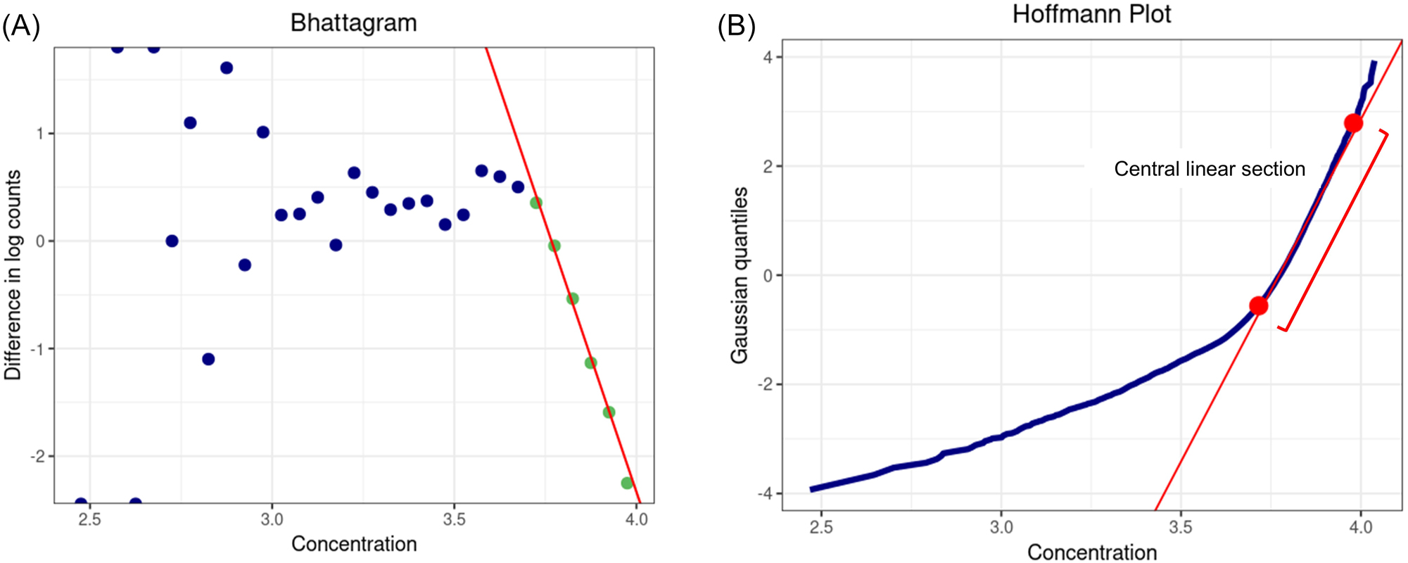
The visualizations of Bhattacharya application (BhattApp) and Hoffmann application (HoffApp) in goCrunch. (A) Bhattagram: the series of green points with a linear downward slope represents the central Gaussian distribution. (B) Hoffmann plot: the red straight line between the lower and upper limits (red dots) represents the central Gaussian distribution.
Hoffmann application (HoffApp)
The HoffApp approach is faithful to the original method of Hoffmann. Notably, it does not use the common variant of the Hoffmann method that plots the cumulative distribution function on an unmodified linear scale, which gives erroneous results [20]. Instead, HoffApp generates a plot equivalent to one produced on normal probability paper using a quantile-quantile plot with a Gaussian comparator distribution. The axes of the plot in HoffApp are transposed compared with usual quantile-quantile plots and this is done to mimic the original Hoffmann method with no impact on the results.
Using a similar approach as in the BhattApp, after filtering and obtaining a normal distribution, the binwidth is automatically created for the histogram (bar graph of “frequency” vs. “concentration”). The optimal binwidth for a given analyte and filtration can be manually selected to create the best histogram. However, in contrast to the Bhattagrams, since the data is not partitioned in the Hoffmann plot (scatter plot of “concentration” vs. “Gaussian quantiles”), adjusting the binwidth does not affect the analysis (Figure 1B). After the construction of the Hoffmann plot, the user determines the lower and upper limits of the straight-line portion representing the Gaussian distribution. After these are marked with dots by the user, the RI is reported.
refineR application
In contradistinction to the aforementioned methods, the analysis is performed without the transformation of data after loading and filtering. In the refineR app, the binwidth is automatically selected for the histogram. Similarly to the HoffApp, the user can manually adjust the binwidth to improve the histogram’s visualization without affecting the RI estimation (Figure 2A).
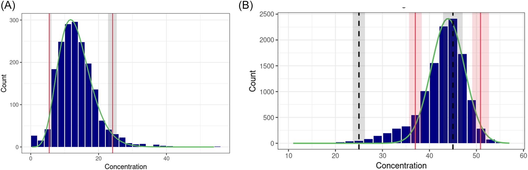
Histogram of the refineR and reflimR applications in goCrunch. (A) refineR: the fitted distribution curve after Box-Cox transformation is shown by the green line, and the estimated reference limits are shown by the red lines. The grey areas show the confidence intervals of the estimated reference limits according to bootstrapping. (B) reflimR: the fitted distribution curve after log transformation is shown by the green line. The estimated reference limit and its permissible uncertainty (pU) are shown by the red lines and areas, respectively. The black dashed lines and grey areas show the target reference limit and its pU, respectively.
The application allows data to be filtered, Box-Cox transformations to be performed automatically, and confidence intervals to be calculated using the bootstrapping technique, all without requiring knowledge of the R language. The user simply needs to specify the number of bootstrap iterations.
reflimR application
There are two application options ‘RefLimR (derive RI)’ and ‘RefLimR (verify RI)’. The first one only estimates RIs, while the second provides verification of the estimated RIs against ‘target values’ (RIs to be verified). Although it doesn’t use traffic light colours for verification as in the reflimR package, it shows the pU in the histogram (Figure 2B) and indicates the acceptability of the verification in the analysis report. This application doesn’t lose speed when calculating confidence intervals because it calculates them with a mathematical equation rather than bootstrapping technique.
ReferenceRangeR
This web tool was developed by the Institute of Clinical Chemistry and Laboratory Medicine at the University of Oldenburg in cooperation with the Section on Guide Limits and Reference Limits of the Deutsche Gesellschaft für Klinische Chemie und Laboratoriumsmedizin (DGKL) in Germany [21].
The web tool’s objective is to facilitate RI estimation with minimal handling efforts, thereby enhancing the accessibility of indirect methods. The tool was developed with the Shiny web application framework [18], and the code was provided on GitHub (github.com/gubruol/ReferenceRangeR/) to enhance transparency and allow users to customize the code for their specific needs. It supports the indirect methods refineR, TMC, TML, kosmic, and reflimR and streamlines the process of stratification. ReferenceRangeR is accessible via a web interface (kc.uol.de/referenceranger/) and available as Docker-based installation for secure local implementation.
Data upload, visualization and stratification
Users can analyze up to 200,000 test results using a simple copy-and-paste process, thereby eliminating the need for file uploads. The visualization and stratification tool generates box plots (median, quartiles and outliers) and violin plots (density distribution) to compare and visualize the data stratified for sex. Differences between the groups are automatically analyzed statistically using the Wilcoxon rank-sum test or Kruskal-Wallis test.
To check for age-related trends (drift), a drift detection algorithm can be performed which supports the user in the identification of age groups characterized by comparable medians. The algorithm groups data into age intervals using an iterative binning procedure. It begins with fine-grained age groups and iteratively merges the two adjacent age groups with the smallest difference in medians. Finally, the maximum deviation of the medians between all remaining groups is calculated and compared to a threshold based on the tolerance intervals of reference limits, which is calculated directly from the dataset, using the pU function described by Haeckel et al. [22]. A smooth additive quantile regression model is applied to derive the median trend and the corresponding confidence intervals. The trend of increasing or decreasing age-related results is visualized.
RI estimation
The tool supports five RI estimation methods (refineR, TMC, TML, kosmic and reflimR), from which the user can choose. It visualizes the estimated RI and the underlying distribution of the selected dataset once the algorithm has been applied to. The analysis report provides information on the indirect method used, the sample size, the age range and gender selection. In addition, a comparison function is implemented to support RI verification. It allows the user to enter a RI for comparison, such as those provided by the manufacturer or an RI obtained using different indirect methods. The two RIs are then compared with each other visually (Figures 3 and 4) and considering the pU [22].
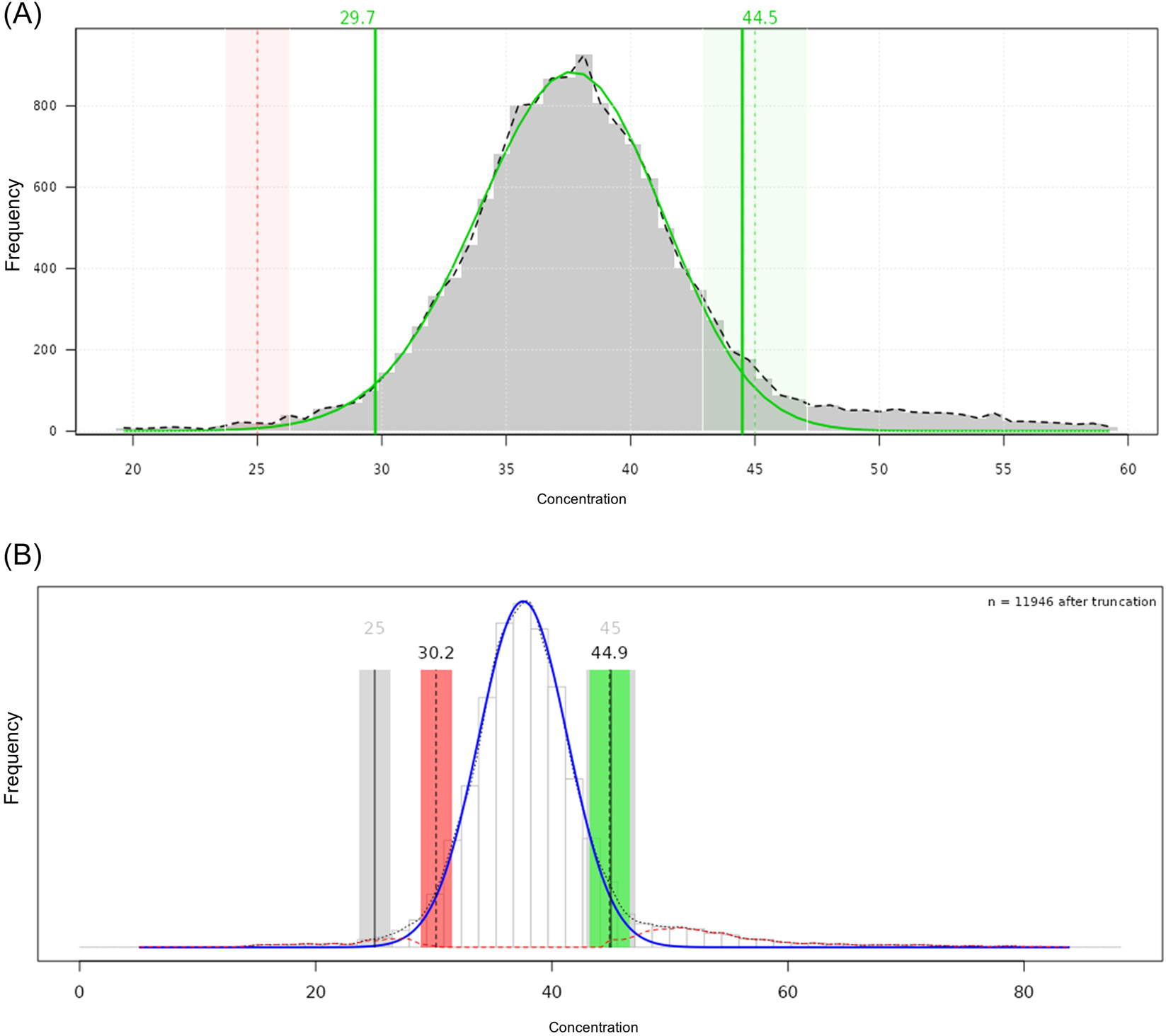
Histogram of the refineR and reflimR applications in ReferenceRangeR. (A) refineR: the fitted distribution curve after Box-Cox transformation and the estimated reference limits are represented with solid green lines (which are vertical for reference limits). The green area shows that the estimated upper limit is within the permissible uncertainty (pU) derived from the target reference limit (vertical dashed green line). The red area shows that the estimated lower limit is outside the pU derived from the target reference limit (vertical dashed red line). (B) reflimR: the fitted distribution curve after log transformation and the estimated reference limits are shown in solid blue and vertical dashed black lines, respectively. A traffic light visualization was used to illustrate agreement between estimated (vertical dashed black lines) and target (vertical solid black lines) reference intervals. A yellow area (not shown here) would indicate that the reference limits are close to or partially outside the pU, requiring careful interpretation of the results. The red area indicates that the reference limits are outside the pU and are therefore unreliable, while the green area shows that the reference limits are within the pU.
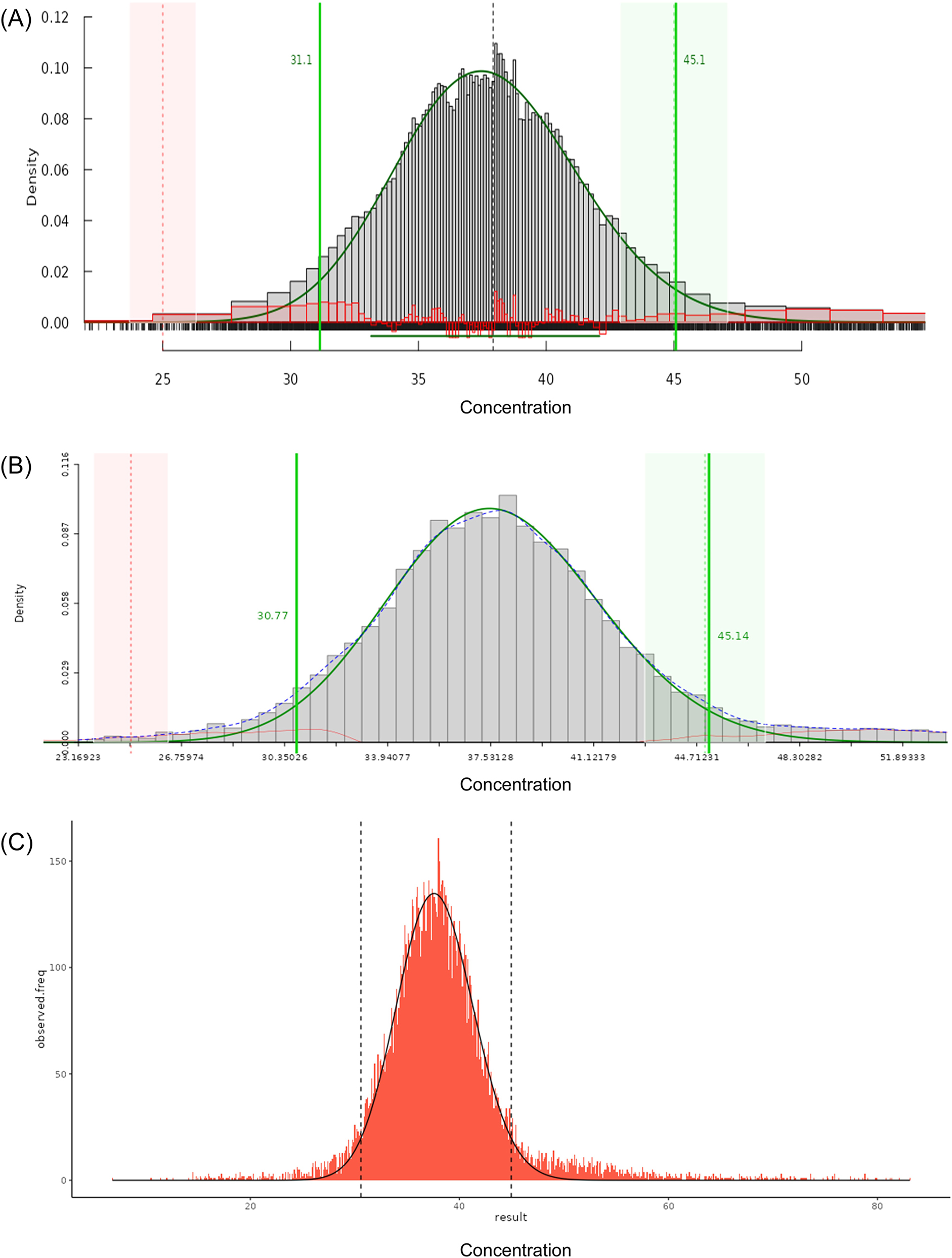
Histogram of the (A) TMC and (B) TML applications in ReferenceRangeR. The fitted distribution curve after Box-Cox transformation and the reference limits are represented with solid green lines (which are vertical for reference limits). The green area shows that the estimated upper limit is within the permissible uncertainty (pU) derived from the target limit (vertical dashed green line). The red area shows that the estimated lower limit is outside the pU derived from the target limit (vertical dashed red line). (C) Histogram of the kosmic application in ReferenceRangeR. The fitted distribution curve after Box-Cox transformation and the reference limits are shown by the solid black and vertical dashed black lines, respectively.
Advanced mode
While the standard mode of the tool is focused on simplicity, the advanced mode provides more functions for selecting individual settings. Users can add trimester information to the data table to perform RI calculation stratified by trimesters of pregnancy and manually adjust the number of age groups using an interactive slider to control the age stratification. TML users can deselect the fast mode to increase the number of significant digits and for the refineR the selection of the modified Box-Cox transformation is provided, as well as the determination of the number of bootstrap replicates (up to a maximum of 50).
Data handling
The applications display warnings and error messages to guide users through the process of estimating RIs. For instance, a warning is displayed if the amount of data is below 2,000 or exceeds 100,000. Furthermore, a warning appears when the labels or abbreviations for the sex need to be assigned manually. The data is automatically cleaned before further processing: Invalid data including negative values or zero as result are removed. This is also applied to data below the limit of quantification (LOQ), except the TMC algorithm, which can handle these results. In cases where data has been cleaned, the number of removed results is displayed in the analysis output.
Data set used for RIs estimation
The two platforms were tested using two sets of RWD with respect to data handling, analysis, and result interpretation. Therefore, anonymized routine laboratory data of platelet count and anion gap (AG) were used. Ethical approval was obtained from the Ethics Committee with decision number 2025-2536 for the platelet count dataset, as well as 2025-199 for the AG dataset.
Incorrect and missing data, as well as values that fell outside the LOQ were removed from both datasets. As there is no gold standard for the comparison of the results obtained by the indirect methods for the datasets used, the mean values from the upper and lower limits, as well as the corresponding pUs were calculated, although it is not known whether the true value is reflected by the mean.
The first example is the platelet count dataset, which is a relatively simple, well-documented analyte whose RIs have frequently been reported in the literature. Furthermore, the analyte has no significant sex or age dependencies for adults. The platelet counts of 86,754 samples collected routinely in the morning from hospital patients aged 20–80 years between July and December 2022 were included.
The second example is the AG dataset, which represents a greater challenge to indirect methods. In addition, it also fills a gap in RI literature. The AG is conventionally reported as [Na+] – ([Cl−] + [HCO3−]), with potassium excluded due to its relatively low plasma concentration and minimal contribution under normal circumstances. This omission has become standard in major textbooks and most clinical practice. Nevertheless, in case of severe hypo- or hyperkalemia the exclusion of potassium can meaningfully shift the calculated AG, potentially obscuring clinically relevant changes [23].
When we sought to establish an appropriate RI for the AG including potassium, we found the published literature to be surprisingly sparse, with mostly outdated references and no consensus across contemporary sources. This motivated us to derive the RI using an indirect approach, which was applied to routine laboratory results (n=15,186) from patients aged 20–80 years between January and June 2025.
Results
The estimated RIs in comparison to the mean values for the reference limits are demonstrated in Figure 5 for the platelet dataset and Figure 6 for the AG dataset, respectively.
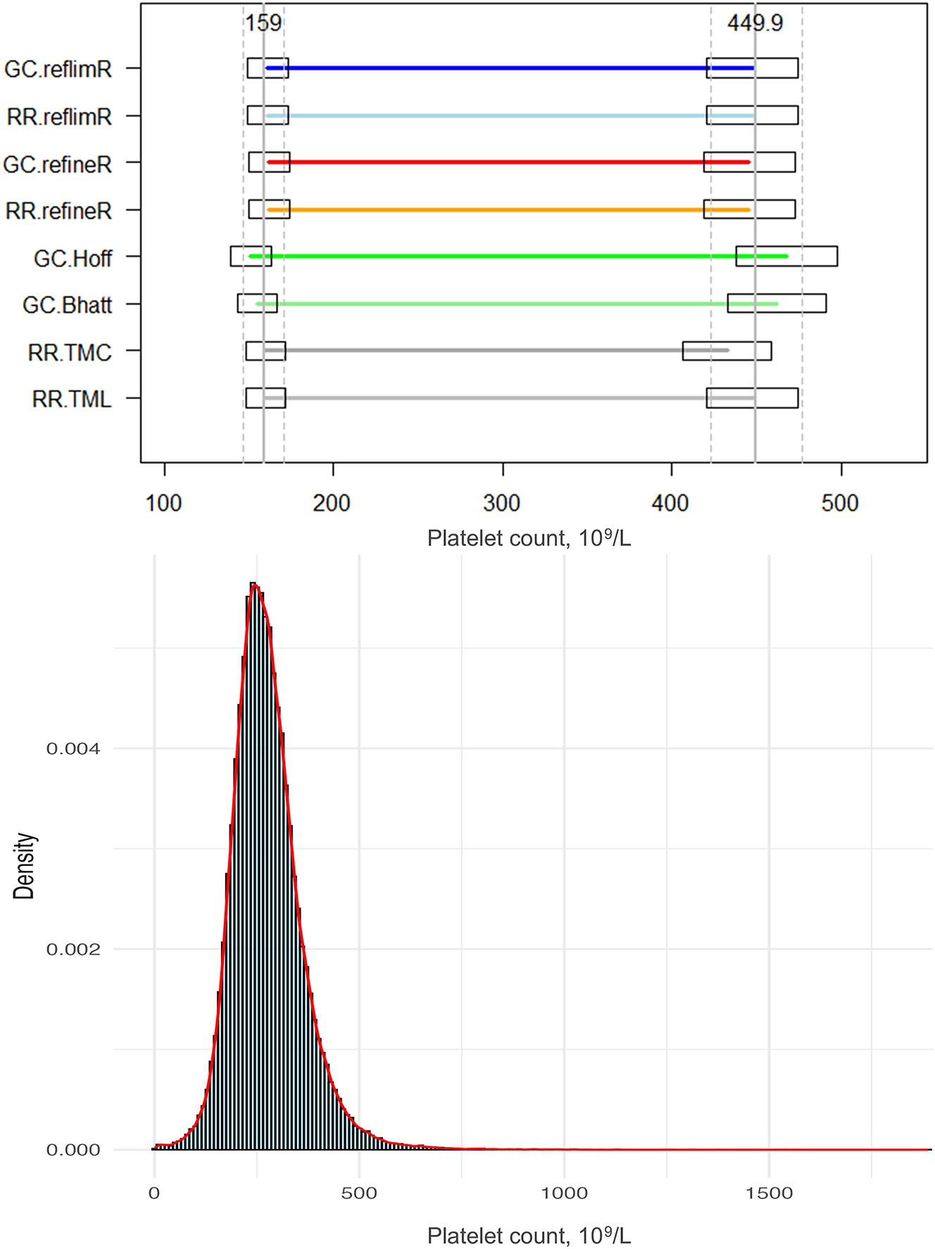
Comparison of the lower and upper reference limits obtained by different indirect methods and the histogram with density curve for the platelet count. Horizontal lines indicate the estimated lower and upper reference limits, while boxes represent the permissible uncertainty (pU). Solid vertical lines denote the mean target values, and dashed lines indicate their pU boundaries.
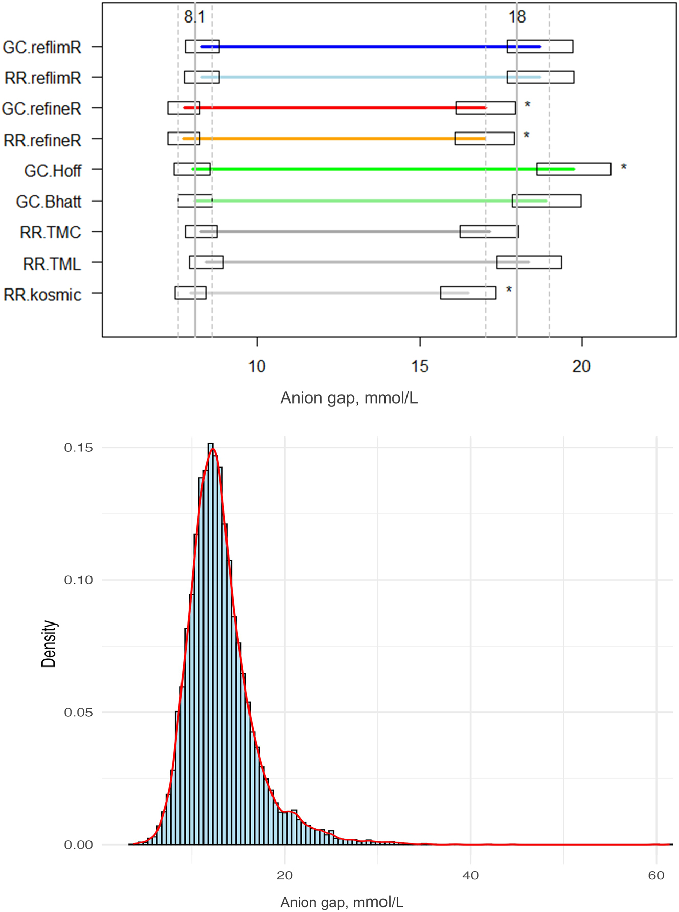
Comparison of the lower and upper reference limits obtained by different indirect methods and the histogram with density curve for the anion gap including potassium. Horizontal lines indicate the estimated lower and upper reference limits, while boxes represent the permissible uncertainty (pU). Solid vertical lines denote the mean target values, and dashed lines indicate their pU boundaries. Asterisks (*) highlight limits falling outside the pU. GC, goCrunch; RR, ReferenceRangeR.
For the platelet dataset, it was found that all methods provided comparable lower limits that were in close agreement with the mean value of 159 × 103/L, with a coefficient of variation (CV) of 2.41 %, exhibiting a range from 151 × 103/L reported by the Hoffmann method, to 161 × 103/L obtained by the reflimR algorithm. The upper limits showed a slightly greater variability, with a CV of 3.54 %. The mean value was found to be 450 × 103/L with the lowest value of 424 × 103/L (refineR) and the highest value of 466 × 103/L (Hoffmann). The reference ranges varied from 272 × 103/L (refineR) up to 315 × 103/L (Hoffmann).
In accordance with the findings of the RI estimations for platelet count, the lower limits obtained from the AG dataset were comparable for all methods, with a mean value of 8.12 mmol/L (CV 2.96 %) and a range from 7.74 mmol/L (refineR) to 8.44 mmol/L (TMC). The upper limits exhibit a greater degree of variability, with a mean value of 18.05 mmol/L and a CV of 6.54 %, with estimated limits ranging from 16.50 mmol/L (kosmic) to 19.74 mmol/L (Hoffmann). The mean width of the RIs was found to be 9.93 mmol/L with a minimum of 8.54 mmol/L (kosmic) and a maximum of 11.73 mmol/L (Hoffmann).
Whilst the Bhattacharya method, the Hoffmann method and the reflimR algorithm utilized a logarithmic transformation, the TMC, TML, kosmic and refineR algotithms performed a Box-Cox transformation with a high variability in the lambda estimations. The lowest lambda value was estimated by TMC with a lambda of 0.45, followed by TML, refineR and kosmic with 0.63, 0.79 and 0.9, respectively.
In both datasets, the methods that performed a Box-Cox transformation estimated narrower RI widths (272 × 103/L to 281 × 103/L for the platelets and 8.54 mmol/L to 9.92 mmol/L for the AG) and thereby lower upper limits. Conversely, the methods that utilized a logarithmic transformation systematically generated wider RIs (285 × 103/L to 315 × 103/L for platelets and 10.39 mmol/L to 11.73 mmol/L for AG) and thereby higher upper limits.
Discussion
Comparison of the RIs estimations for different datasets
Both datasets were slightly skewed (1.76 for AG vs. 1.41 for platelets) and heavy-tailed (kurtosis of 7.83 for AG and 8.23 for platelets).
While the platelet dataset served as an illustrative example of an analyte with no apparent age- or sex-related dependencies, providing an opportunity to assess the performance of different indirect approaches under relatively simple conditions. The dataset of AG including potassium appears to be a more complex example as its distribution has a plateau at about 20 mmol/L, which might indicate overlapping subpopulations. Furthermore, the AG dataset may contain mixed distributions, as indicated in the density curve (Figure 6). This may be the reason for the highest variability observed for the upper limits of AG with a CV of 6.54 %.
While the estimations of the lower limits of the different indirect methods were comparable in both datasets, the upper limits had higher variability. Given that the sample sizes of both datasets are considered large enough for all the indirect methods used, the observed variety might be attributable to the heavy-tailed, right-skewed data distributions and the different approaches used for transformation on the one hand and the different ways of dealing with pathological values on the other hand, especially in cases where subpopulations overlap, as in the AG dataset.
The methods using a Box-Cox transformation have shown differences in the estimation of lambda, which may explain the variability between the RIs estimated by these methods, as it is a known weakness of Box-Cox based methods that may specify a lambda value that is too high/low or do not fit to the assumed log-normal distribution. The fact that the estimated RIs for both datasets had higher widths and higher upper bounds in the logarithmic transformation compared to the Box-Cox transformation may be due to differences in handling the heavy-tailed data distribution.
The overlapping of diseased and non-diseased subgroups is one of the most challenging problems when using indirect methods, as so far there is no clear methodology for discrimination between those subpopulations. In this case, various machine learning algorithms can be used to separate mixed distributions with high levels of pathological data or those requiring partitioning, based on factors such as age and gender [24], 25].
The mean RI for the AG derived by indirect approaches was consistent with the literature review [26], 27], when adding an expected potassium concentration to the published RIs from the AG without potassium. In our view, this example highlights a use case for RI estimation. Indirect methods may be a reliable and pragmatic strategy to establish RIs when classical reference population studies are not possible and adequate RIs from literature are not available.
The benefits and drawbacks of the indirect methods
The Hoffmann and Bhattacharya methods strongly rely on Gaussian distributed datasets, while laboratory data is often skewed. The goCrunch website provides a platform for users to implement the requisite transformation on their respective datasets. Although the BhattApp and the HoffApp facilitate their utilization, both methods rely on visual decisions made by the user, which is therefore highly subjective. Furthermore, both methods only work reliably if a reasonably straight line can be drawn from one end of the graph to the other [15]. If the graph consists of two distinct subgroups with different regression lines, the methods will inevitably be flawed. Consequently, the reliability and consistency of the results are contingent on the user’s expertise, particularly in data handling with different distributions.
Among the more recent methods, reflimR is the only algorithm that does not rely on lambda estimation for Box-Cox transformation. A distinct advantage of this method is the shortest computational time, but its reliability is compromised in cases where the distribution is neither normal nor lognormal. Nonetheless, reflimR it is easily interpreted thanks to the traffic light color metaphor.
A key advantage of refineR is its ability to identify a distribution reflecting healthy individuals, by estimating the most appropriate lambda value without manual intervention. Another advantage of refineR is that it can calculate confidence intervals for RI estimates using the bootstrapping method. However, the disadvantage of bootstrapping is that the calculation time increases significantly, as the algorithm must be rerun many times.
Firstly, reflimR can be used for the verification of RIs, as it is extremely fast and provides easily interpretable results thanks to the traffic light color metaphor. If yellow or even red traffic lights are displayed, an estimation with refineR to validate the RIs of reflimR may be recommended. If both methods yield consistent results, it can be assumed that the target value needs to be corrected. If they do not match, it is more likely that the data set used is too complex for analysis with indirect methods. An analysis that discriminates between overlapping subfractions cannot be performed by either platform. In this case, a distribution decomposition program such as mclust or mixtools may be used to eventually identify the cause of the complexity [28]. So, there is still need for medical and statistical expertise when estimating RIs by indirect methods.
The TMC has been developed to manage highly skewed data distributions, and it offers the distinct advantage of being able to process values below the quantification limit. Therefore, only the TMC can be used to estimate RIs for such datasets.
Despite the aforementioned specific benefits and drawbacks, the key advantage of all recent methods (TMC, TML, kosmic, reflimR and refineR) is the capacity for their execution to be entirely automated, with minimal or no statistical expertise, as demonstrated by both ReferenceRangeR and goCrunch.
The general concordance across approaches supports the utility of indirect strategies in establishing RIs, particularly when traditional reference population studies are impractical. However, the role of expert judgment remains essential to ensure that statistical outputs are both methodologically sound and clinically meaningful.
Conclusions
The development of user-friendly platforms such as goCrunch and ReferenceRangeR marks a significant advancement in the field of indirect RI estimation. Both tools reduce the complexity traditionally associated with statistical programming in R, thereby making advanced RI estimation methodologies more accessible and supporting in meeting accreditation and quality requirements to laboratory professionals.
goCrunch provides a practical entry point with classical and modern algorithms, intuitive visualization, flexibility for data preprocessing, and a verification application using reflimR, making it particularly suitable for routine laboratory use and education. ReferenceRangeR, on the other hand, offers a broader spectrum of advanced statistical approaches, enhanced stratification options, automated drift detection of age, and comparative functionalities for each method. Despite differences in their capacities and focus, both tools improve the reliability and reproducibility of indirect RI estimation. Future updates expanding automation, multi-analyte analysis, and report generation will further strengthen their role as essential tools in clinical laboratory medicine.
In conclusion, goCrunch and ReferenceRangeR complement each other by bridging the gap between methodological sophistication and practical usability. Their widespread adoption will not only promote standardization and quality in RI determination but also empower clinical laboratories to make more accurate, efficient, and patient-centered decisions.
-
Research ethics: Ethical approval was obtained from the Ethics Committee with decision number 2025-2536 for the platelet count dataset, as well as 2025-199 for the AG dataset.
-
Informed consent: Not applicable.
-
Author contributions: FDA contributed to the design of the study, to providing the data, to executing the experiments, to the interpretation of the results, and drafted and reviewed the article. CF, GB and MV contributed to providing the data, to executing the experiments, to the interpretation of the results, and drafted and reviewed the article. ACY drafted and reviewed the article. All authors have accepted responsibility for the entire content of this manuscript and approved its submission.
-
Use of Large Language Models, AI and Machine Learning Tools: None declared.
-
Conflict of interest: The authors state no conflict of interest.
-
Research funding: None declared.
-
Data availability: Not applicable.
References
1. CLSI. Defining, establishing, and verifying reference intervals in the clinical laboratory, 3rd ed. Wayne, PA: Clinical and Laboratory Standards Institute; 2010. (CLSI document C28-A3C).Search in Google Scholar
2. Graesbeck, R. The evolution of the reference value concept. Clin Chem Lab Med 2004;42:692–7. https://doi.org/10.1515/cclm.2004.118.Search in Google Scholar
3. International Organization for Standardization. ISO 15189: 2022 Medical laboratories: requirements for quality and competence. Geneva: ISO; 2022.Search in Google Scholar
4. Solberg, HE. Approved recommendation on the theory of reference values. Part 1. The concept of reference values. Clin Chim Acta 1987;165:111–8. https://doi.org/10.1016/0009-8981(87)90224-5.Search in Google Scholar PubMed
5. Jones, GR, Haeckel, R, Loh, TP, Sikaris, K, Streichert, T, Katayev, A, et al.. Indirect methods for reference interval determination – review and recommendations. Clin Chem Lab Med 2018;57:20–9. https://doi.org/10.1515/cclm-2018-0073.Search in Google Scholar PubMed
6. Hoffmann, RG. Statistics in the practice of medicine. JAMA 1963;185:864–73. https://doi.org/10.1001/jama.1963.03060110068020.Search in Google Scholar PubMed
7. Bhattacharya, CG. A simple method of resolution of a distribution into Gaussian components. Biometrics 1967;23:115–35. https://doi.org/10.2307/2528285.Search in Google Scholar
8. Arzideh, F, Wosniok, W, Gurr, E, Hinsch, W, Schumann, G, Weinstock, N, et al.. A plea for intra-laboratory reference limits. Part 2. A bimodal retrospective concept for determining reference limits from intra-laboratory databases demonstrated by catalytic activity concentrations of enzymes. Clin Chem Lab Med 2007;45:1043–57. https://doi.org/10.1515/cclm.2007.250.Search in Google Scholar
9. Arzideh, F. Estimation of medical reference limits by truncated Gaussian and truncated power normal distributions [Doctoral dissertation]. Bremen Univ Diss; 2008.Search in Google Scholar
10. Wosniok, W, Haeckel, R. A new indirect estimation of reference intervals: truncated minimum chi-square (TMC) approach. Clin Chem Lab Med 2019;57:1933–47. https://doi.org/10.1515/cclm-2018-1341.Search in Google Scholar PubMed
11. Zierk, J, Arzideh, F, Kapsner, LA, Prokosch, HU, Metzler, M, Rauh, M. Reference interval estimation from mixed distributions using truncation points and the Kolmogorov-Smirnov distance (kosmic). Sci Rep 2020;10:1704. https://doi.org/10.1038/s41598-020-58749-2.Search in Google Scholar PubMed PubMed Central
12. Ammer, T, Schützenmeister, A, Prokosch, HU, Rauh, M, Rank, CM, Zierk, J. refineR: a novel algorithm for reference interval estimation from real-world data. Sci Rep 2021;11:16023. https://doi.org/10.1038/s41598-021-95301-2.Search in Google Scholar PubMed PubMed Central
13. Hoffmann, G, Klawitter, S, Trulson, I, Adler, J, Holdenrieder, S, Klawonn, F. A novel tool for the rapid and transparent verification of reference intervals in clinical laboratories. J Clin Med 2024;13:4397. https://doi.org/10.3390/jcm13154397.Search in Google Scholar PubMed PubMed Central
14. Ying, Z, Weibo, M, Guocheng, W, Yaqi, L, Yaguang, P, Xiaoxia, P. Limitations of the Hoffmann method for establishing reference intervals using clinical laboratory data. Clin Biochem 2019;63:79–84. https://doi.org/10.1016/j.clinbiochem.2018.11.005.Search in Google Scholar PubMed
15. Hoffmann, G, Lichtinghagen, R, Wosniok, W. Simple estimation of reference intervals from routine laboratory data. J Lab Med 2015;39:389–402. https://doi.org/10.1515/labmed-2015-0104.Search in Google Scholar
16. Klawonn, F, Riekeberg, N, Hoffmann, G. Importance and uncertainty of λ-estimation for Box-Cox transformation to compute and verify reference intervals in laboratory medicine. Stats 2024;7:172–84. https://doi.org/10.3390/stats7010011.Search in Google Scholar
17. Agaravatt, A, Kansara, G, Khubchandani, A, Sanghani, H, Patel, S, Parchwani, D. Verification of reference interval of thyroid hormones with manual and automated indirect approaches: comparison of hoffman, KOSMIC and refineR methods. Cureus 2023;15:e39066. https://doi.org/10.7759/cureus.39066.Search in Google Scholar PubMed PubMed Central
18. Chang, W, Cheng, J, Allaire, J, Sievert, C, Schloerke, B, Xie, Y, et al.. Shiny: web application framework for R [Internet]. Version 1.11.1.9000; 2025. Available from: https://CRAN.R-project.org/package=shiny.Search in Google Scholar
19. Røys, EÅ, Viste, K, Kellmann, R, Guldhaug, NA, Alaour, B, Sylte, MS, et al.. Estimating reference change values using routine patient data: a novel pathology database approach. Clin Chem 2025;71:307–18. https://doi.org/10.1093/clinchem/hvae166.Search in Google Scholar PubMed
20. Holmes, DT, Buhr, KA. Widespread incorrect implementation of the Hoffmann method, the correct approach, and modern alternatives. Am J Clin Pathol 2019;151:328–36. https://doi.org/10.1093/ajcp/aqy149.Search in Google Scholar PubMed
21. Brandhorst, G, Voß, M, Wosniok, W, Arzideh, F, Haeckel, R, Rosenkranz, D, et al.. Reference RangeR: a novel tool designed to facilitate reference interval estimation and verification. Clin Chem Lab Med 2025. https://doi.org/10.1515/cclm-2025-0637 [Epub ahead of print].Search in Google Scholar PubMed
22. Haeckel, R, Wosniok, W, Arzideh, F. Equivalence limits of reference intervals for partitioning of population data. Relevant differences of reference limits. J Lab Med 2016;40:199–205. https://doi.org/10.1515/labmed-2016-0002.Search in Google Scholar
23. Kraut, JA, Nagami, GT. The serum anion gap in the evaluation of acid-base disorders: what are its limitations and can its effectiveness be improved? Clin J Am Soc Nephrol 2013;8:2018–24. https://doi.org/10.2215/cjn.04040413.Search in Google Scholar
24. Hoffmann, G, Allmeier, N, Kuti, M, Holdenrieder, S, Trulson, I. How Gaussian mixture modelling can help to verify reference intervals from laboratory data with a high proportion of pathological values. J Lab Med 2024;48:251–8. https://doi.org/10.1515/labmed-2024-0118.Search in Google Scholar
25. Klawitter, S, Böhm, J, Tolios, A, Gebauer, J. Automated sex and age partitioning for the estimation of reference intervals using a regression tree model. J Lab Med 2024;48:223–37.10.1515/labmed-2024-0083Search in Google Scholar
26. Rifai, N, Horvath, AR, Wittwer, C, Tietz, NW, editors. Tietz textbook of clinical chemistry and molecular diagnostics, 6th ed. St. Louis, MO: Elsevier; 2018:1867 p.Search in Google Scholar
27. Berend, K, de Vries, AP, Gans, RO. Physiological approach to assessment of acid-base disturbances. N Engl J Med 2014;371:1434–45. https://doi.org/10.1056/nejmra1003327.Search in Google Scholar
28. Arslan, F, Hoffmann, G. Use of indirect methods and machine learning algorithms for the estimation of reference intervals, taking cortisol measurements as an example. Clin Chem Lab Med 2025. https://doi.org/10.1515/cclm-2025-0984 [Epub ahead of print].Search in Google Scholar PubMed
© 2025 the author(s), published by De Gruyter, Berlin/Boston
This work is licensed under the Creative Commons Attribution 4.0 International License.
Articles in the same Issue
- Frontmatter
- Editorial
- Entering a new era of laboratory data processing and interpretation
- Articles
- Sustainable reference intervals and decision limits
- An update to reflimR: strengthening transparent reference interval verification
- Intuitive web tools for reference interval estimation: goCrunch and ReferenceRangeR
- Automated age and sex partitioning of reference intervals based on routine laboratory data
- Using zlog in spider charts for fast diagnosis recognition
- Using large language models for therapeutic drug monitoring reporting – a proof-of-concept
- EU AI Act: what could AI literacy mean for medical laboratories? – Opinion Paper on behalf of the Section Digital Competence and AI of the German Society for Clinical Chemistry and Laboratory Medicine (DGKL)
- Annual Reviewer Acknowledgment
- Reviewer Acknowledgment