Climate Change Risks and Consequences on Growth and Debt-Sustainability in Africa
-
John Asafu-Adjaye


Abstract
Average temperature in Africa has been rising steadily from the baseline of climatology prevailing during 1951–1980. The findings in this paper suggest that real GDP growth would start declining for annual temperature higher than 0.7 °C. About 45 African countries already registered annual temperature rise above 0.7 °C in 2020 underscoring the seriousness of climate change induced risks for long term growth. In addition, frequency of major natural disasters tends to exacerbate political instability and conflict. Combined, these shocks have a direct effect on the sustainability of debt. Using a simple debt dynamics framework, the paper shows that the debt-burden could increase 2.4 times due to climate change induced shocks. In addition, modelling results show that carbon pricing could be an effective way of helping to meet the Nationally Determined Contributions. However, carbon pricing would have negative impacts on energy-intensive industries and increase the prices of the goods and services they provide. There will also be job losses in these industries. The combined effect of these impacts could be reduction in GDP growth and real incomes. It is recommended that part of the revenues generated from the carbon tax could be used to address the negative impacts on vulnerable groups.
1 Introduction
There is no denying that we are at the cusp of experiencing climate change induced catastrophe that could be irreversible. The time is ticking for any meaningful action to make a difference. The transition to green energy sources is needed with urgency and scale to stem the risk of climate change related shocks. The main challenge is the enormous cost to the world economy which for centuries has relied on energy sources derived from fossil fuel, such as oil and gas, coal and others that polluted the environment through the CO2 emissions. A recent publication of the International Energy Agency estimated in its World Energy Outlook, 2021[1] that over US$30 trillion is needed up to 2030 for a green transition to take place effectively across the globe. Certainly, affordable technology in renewable energy sources is progressing rapidly, making the outlook to green transition hopeful. On the other hand, energy prices are rising despite diversified energy sources, partly due to ever rising energy demand, and at the same time regulated energy markets largely driven by geo-political considerations.
Although Africa has contributed only 3.8 % of total global emissions, it has borne the brunt of climate change. Annually, Africa loses US$7–$15 billion due to climate change (Adesina 2021). This figure is expected to rise to US$50 billion by 2040. The $100 billion per year climate financing pledged at COP21 in Paris in 2015 has not yet materialized. Going into COP26 in 2021, the African Group of Negotiators had pushed for African climate mitigation and adaptation funding to be scaled up to US$1.3 trillion per year by 2030, to be split 50:50 between adaptation and mitigation funding. This target was not achieved, although rich countries pledged to double adaptation funding by 2025 which would amount to about US$40 billion per year. While this is an improvement on current funding levels, it is still insufficient to achieve an equal split between adaptation and mitigation. The current financing levels fall short of Africa’s needs by US$100–$127 billion per year from 2020 to 2030. Some African countries are already spending more on climate adaptation than on health care and education.
Four out of five people in the world without energy access live in Sub-Saharan Africa (SSA), impeding industrialization and development. Consequently, Africans must balance the need to combat climate change with an urgency to develop the continent’s economies to alleviate hunger and poverty, among other UN Sustainable Development Goals. SDG7 – affordable and clean energy – remains out of reach for half of Africa’s people and is key to unlocking the other 16 goals. Development of transport and logistics, and technology infrastructure is also vital. The evidence suggests that Africa contributes less than 3 % of total global greenhouse gas (GHG) emissions yet suffers the most from climate change shocks. The main factors that exposed African countries to climatic shocks include the source of livelihood, which is predominantly from agriculture that on the average employs over 55 % of the work force and contributes close to 20 % of GDP.[2] This suggests the low productivity pervading the sector where over 95 % of farming relies on rain-fed agriculture and is prone to extreme weather variability. As a result, seven of the 10 most vulnerable countries to climate shock in the world are in Africa.
The AERC’s research[3] in this area shows that higher temperatures, coupled with reduced and/or variable rainfall, could lead to reduced agricultural output which will be transmitted to domestic prices and inflation. This can happen in several ways. First, the negative impact on agricultural productivity will contribute to food shortages, causing food prices to rise when there is an excess of demand over supply. This is more likely in countries where the foreign exchange reserve and fiscal space is very weak to establish buffer against severe drought, flood, or other sources of crop failures including locust attacks such as experienced recently in the horn of Africa.
Second, climate shocks could translate into higher prices through trade as most African countries depend on primary commodities for their exports. Export contractions and likely import expansion could lead to weaking of exchange rate, hence drive domestic prices upwards, especially in situations of fixed exchange rates regimes. Finally, droughts in the horn of Africa will affect food prices and energy prices due to dependence on hydroelectricity generation. A combination of food and energy prices is a major supply shock on inflation. Monetary policy instruments in these countries do not have supply side instruments to mitigate these effects. Without any buffers on food or energy, these countries end up using demand side instruments to dislodge the effects of a plateau of high prices and thus plunge the economy into a short-term recession.
As Africa envisages to build a climate shock resilient economy through industrial policies and other strategies of automation, the energy demand is likely to accelerate which requires a careful approach to mitigation and adaptation methods. Currently over 80 % of Africa’s energy consumption is generated from natural gas, coal, and oil, which are fossil-fuel based and contribute to greenhouse effects. The rest is accounted for by hydro, solar PV, geothermal, solar thermal and biofuel that are green and renewable sources of energy.[4] In addition, close to 20 % of African countries are exporters of oil on which their economy depends for foreign exchange earnings, government revenue and employment. Hence, transitioning to green and renewable energy sources will come at a heavy cost. It is also important to note that Africa’s consumption of energy is the lowest in the world. The percentage of households that have access to electricity is less than 40 % at the continental level, with the situation even worse in rural areas. It is difficult to imagine rural transformation without access to reliable and adequate energy.
Studies have shown that rural electrification in Africa is not an easy fit even when there is strong government commitment. Most households cannot not afford to be connected to the grid and even if they do through some government subsidizes, they sparingly consume electricity because they cannot afford the bills, their income flows are low and erratic. The median price of electricity in 2021 in Africa is over 30 % higher than the world average. In some African countries, the difference is over 200 %. This simply suggests the need for a relatively cheaper and abundant source of energy to realize Africa’s economic transformation. Certainly, many African countries have potential for hydro, wind, and solar energy because of the geography.
This study uses a combination of econometric modelling, debt dynamics analysis, and computable general equilibrium (CGE) modelling to explore the effects of climate change on growth, debt, and sectoral output in Africa, and to address the policy implications. The rest of the paper is organized as follows. Section 2 presents the challenges of climate change and its effect on economic growth, political stability and conflict and fiscal deficit. Section 3 uses the effect from reduced real GDP growth and budget deficit to estimate debt trajectories. Section 4 explores the transition to low-carbon economy, while Section 5 concludes.
2 Climate Risks and Shocks in Africa: Overview
2.1 Real per Capita GDP Growth and Rising Temperature in Africa
One of the indicators of climate change that causes extreme weathers, such as drought, flooding and other shocks is a rise in average temperature over time. Figure 1 below presents trends in the change in average temperature for the period 1990–2021 from the baseline of climatology prevailing in the 1950s.
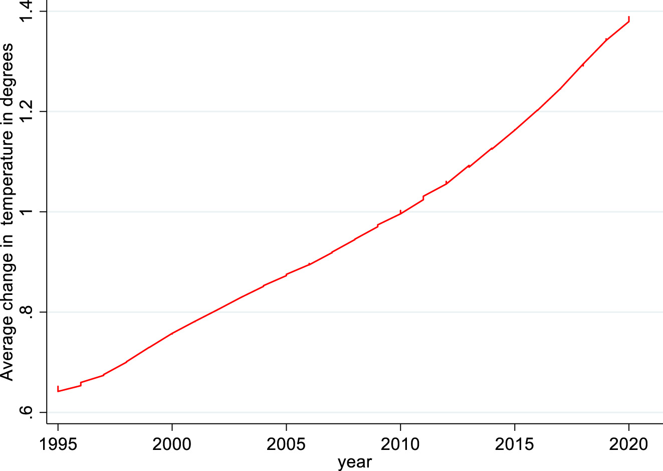
Average temperature change in degree centigrade in Africa. The annual temperature change is computed from the climatology that prevailed during 1951–1980. Source: Authors’ computations based on data from FAOSTAT.
Average temperature has been rising rapidly and steadily in Africa crossing the one-degree centigrade mark in 2010. If the situation continues untamed, the disruptions that could follow on the economy could be significant. We also note that there is significant heterogeneity across countries in their exposure to rising temperature. The literature that assesses the impact of climate change on real GDP growth in Africa is limited, though growing. For example, Baarsch et al. (2020) reported that due to unequal exposure to climate-induced shocks, long-term growth in Africa could create different convergence clubs, further aggravating inequalities in the continent.[5] Their results suggest that up to 15 % of GDP per capita growth could be lost due to climate induced risks. Also, Abidoye and Odusola (2015) found that for the period 1960–2009, rise in temperature beyond 1 °C could lead to reduction in real GDP growth by about 0.67 percentage points. In this study, we update this literature using the most recent data (1990–2021) and decomposing real GDP growth into cyclical and long-term component. The linear model we estimated is specified as follows:
Where g it stands for real GDP growth, T it for annual change in temperature from baseline, and its square (T it 2) and X it are control variables that include political stability and quality of institutions. The error terms control for time-variant and time-invariant unobserved factors. Equation (1) was estimated using a fixed-effects panel data regression method and results are reported in Table 1 below.
Effect of temperature change on real per capita GDP growth in Africa, 1990–2021.
| Dependent variable | |||
|---|---|---|---|
| Explanatory variables | Real per capita GDP growth | Cyclical real per capita GDP growth | Long term real per capita GDP growth |
| Lag change in temperature | 0.0209 | 0.0186** | 0.00231 |
| (1.4) | (2.93) | −0.16 | |
| Squared lag change in temperature | −0.0119 | −0.01** | −0.00304 |
| (−1.71) | (−3.00) | (−0.46) | |
| Constant | 0.0229 | 0.00766 | 0.0152 |
| (1.89) | (1.49) | (1.32) | |
| Political economy controls | Yes | Yes | Yes |
| Country and year fixed effects | Yes | Yes | Yes |
| Number of countries | 51 | 51 | 51 |
| Observations | 990 | 990 | 990 |
| Overall R-square | 0.061 | 0.062 | 0.051 |
| Within R-square | 0.02 | 0.01 | 0.01 |
| Between R-square | 0.10 | 0.02 | 0.08 |
-
1. Real GDP growth is decomposed into cyclical and long-term component using the Kalman filter. 2. Temperature data reflects annual change in degrees from the baseline of climatology prevailing during 1951–1980. Political economy control factors include: rule of law, political stability and macroeconomic stability (inflation). From column 1 and 2, real GDP growth would start declining for annual temperature changes starting at 0.7 °C. 3. t-statistics in parentheses: *p < 0.05, **p < 0.01, ***p < 0.001.
According to the table, real GDP growth responds negatively to a rise in temperature beyond a certain level. Most importantly, climate shock generally is highly correlated with the cyclical component of GDP growth rather than the long-term trend, which suggests that part of the volatility observed in growth emanates from climate-induced shocks. Column 2 of Table 1 suggests that a 0.7 °C rise in annual temperature could lead 2 percentage points decline in real GDP growth, undermining positive shocks, such as commodity price booms, and amplifying negative shocks. It may have to be noted that the relationship between rise in temperature and real GDP growth reinforce each other, hence identification of the causation requires specifying structural econometric model. To reduce some potential endogeneity issues, the regression reported in Table 1 used one year-lagged annual change in temperature in degree centigrade. The working hypothesis is that rising temperature causes extreme weather such as drought, floods and other forms of natural disasters that could disrupt livelihoods and affect economic activities (Table 2).
Effect of annual temperature change on growth: system GMM estimation.
| Explanatory variables | Per capita GDP growth | Cyclical real per capita GDP growth | Long term real per capita GDP growth |
|---|---|---|---|
| Lagged per capita GDP growth | −0.084 | 0.317 | −0.220 |
| (−2.72)** | (10.54)*** | (−7.26)*** | |
| Lagged temperature | 0.824 | 0.009 | 0.012 |
| (−0.48) | (1.89) | −0.94 | |
| Lagged temperature squared | −1.56 | −0.01 | −0.01 |
| (−1.95) | (−2.24)** | (−1.12) | |
| Sargan’s overidentification test | 0.000 | 0.177 | 0.000 |
| Number of observations | 932 | 932 | 932 |
-
Table reports the Arellano-Bond two step (system) GMM estimation and controls for heteroscedastic errors. t-statistics in parentheses: *p < 0.05, **p < 0.01, ***p < 0.001.
In addition, as a robustness test to the results reported in Table 1, a linear dynamic panel model was estimated where per capita GDP growth is assumed to exhibit state dependence. The two-step system Generalized Method of Moments (GMM) was used to control for potential endogeneity between the unobserved time-invariant error terms and per capita GDP growth. Internal instruments (lagged annual temperature change and its square, quality of institutions and year dummies) were used to address endogeneity issues. The results suggest that the overidentifying restrictions of instruments is valid only for the cyclical component of per capita GDP growth, and invalid for per capita GDP growth and long-term per capita GDP growth. Furthermore, the results indicate that annual changes in temperature impacts per capita GDP growth negatively at higher degree of warming confirming the result reported in Table 1. Similarly, no significant correlation was observed between per capita GDP growth and long-term per capita GDP growth on the hand and annual change in the average temperature on the other. It can be noted that the negative coefficient associated with the lagged dependent variables (per capita GDP growth and long-term per capita GDP growth) may suggest the possibility of convergence within African economies (initially low-income countries growing faster than high income countries). Also, the positive coefficient associated with the cyclical per capita GDP growth suggests the propagation and persistence of shocks over time. In summary, there is strong association between cyclical component of per capita GDP growth and rising temperature.
Figure 2 clearly shows that in 2020 nearly 45 countries in Africa experienced annual temperature rise above the threshold of 0.7 °C. Computations show that the annual average trend has been 0.03 °C on the average and Africa is expected to hit 1.8-°C rise in average change in temperature by 2030.
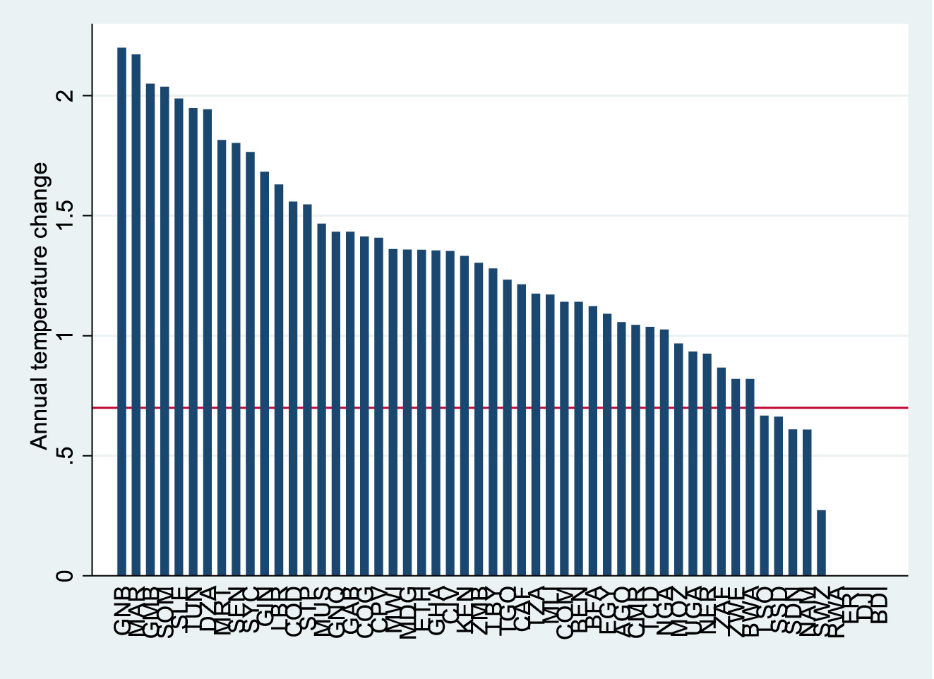
Average annual change in temperature by country in Africa: 2020. The figure presents by country annual change in average temperature in 2020 and marks the threshold of 0.7 °C beyond which real GDP growth starts to decline.
It is also feasible to identify an indirect channel. Natural disasters tend also to increase competitions for resources, such as water and fertile land among communities, creating conditions for political instability and conflict. In this regard, the risk of climate-change induced risk poses a significant threat to the long-term development of Africa.
Figure 3 presents the correlation between the number of major natural disasters recorded in Africa every year since the 1990s and incidence of conflict and political instability. Countries that suffered frequent natural disasters also exhibited high incidence of violence and political instability. This is an important channel through which economic activity could be disrupted by climate change induced natural disasters. Preliminary correlations showed that a 1 % increase in per capita CO2 emissions is correlated with around 0.75 % increase in natural disasters further solidifying the link between natural disasters and climate change.
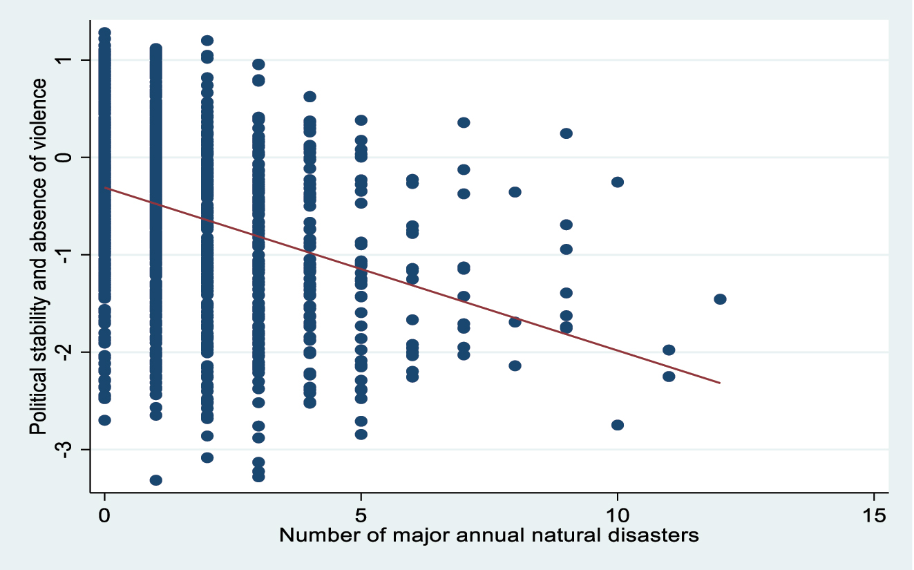
Number of major natural disasters and political instability/conflict in Africa. Source: Authors’ computations based on data from World Development Indicators.
In addition, the correlation between a country’s emission of CO2 per capita and annual temperature change is positive and significant (Figure 3). This is indicative of reinforcing processes where higher CO2 emissions go hand in hand with rise in the average temperature which has detrimental effect on long-term growth beyond a certain threshold (Figure 4).
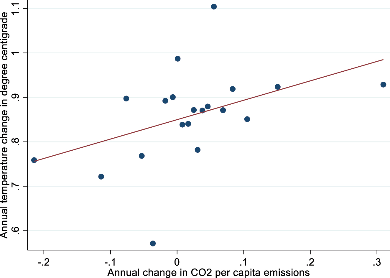
Bin-scattered diagram on the correlation of annual temperature change and CO2 per capita emissions in Africa. Figure 4 controls for economic structure (share of manufacturing and agriculture in GDP), energy consumption and political economy factors.
3 Climate Shocks on Debt Trajectories
3.1 Methodology: Understanding Debt Dynamics
In this section, a simple debt dynamics model is used to motivate the discussion on designing an optimal debt management strategy. Consider the following well known definition of debt dynamics:[6]
Where D t is total debt stock in either local or international currency, r is the average interest rate on the debt, and PB t is total primary balance of the government budget that require current financing. Deficits in government budget add to the debt stock, while surpluses reduce it. Dividing through by GDP t, and rearranging we get:
Where g is growth in nominal GDP and small letters indicate same variables as share of GDP.
Equation (3) is basically an identity, but the dynamic specification provides rich information on conditions for the stability of debt overtime. In addition, some of the drivers of debt, particularly that of external debt have interesting features that allow decision makers to plan and understand better the path of debt. For instance, interest rate, especially for external debt is quasi-exogenous. Some of which could be concessional as often the case is and beyond the control of the policy makers. On the other hand, the cost of borrowings from the capital market tends to be influenced by credit rating agencies whose assessment of the country’s credit worthiness depends on factors that considers global economic conditions as well as the opportunities afforded and perception of risks in the country, hence partly endogenous. GDP growth rate is endogenous shaped by economic fundamentals, institutions, and policy except for transitory shocks. Government budget is policy driven where spending and revenue mobilizations are shaped by public administration, and intertemporal consumption preferences of the government, including the discount rate for current spending. Impatient and short-sighted governments tend to accumulate debt rapidly compared with those that have long-term perspectives.
Hence, even though the decision to borrow is ultimately dependent on policy makers, not everything is under their control when it comes to the speed of debt accumulation and implications to the overall economy.
From Equation (3), some characterization of the dynamics of debt can be made. For example, if the economy grows (g t) at the same pace as the cost of borrowing (r t), then, debt burden grows by the full amount of the government budget deficit. The only way debt can be contained is if the government budget experiences a surplus or the budget is fully balanced (zero budget deficit). If the economy grows faster than cost of borrowing, or interest rate on the loan, then, the country can continue to run budget deficits without experiencing explosive debt trajectory. If the economy grows much less than the interest rate, then, debt burden increases explosively, and the country needs to run a budget surplus not to buckle under the burden. Hence, economic contraction, caused for instance by significant shocks such as COVID-19 can aggravate debt-burden beyond the short-term. The solution therefore to the difference equation (2) that determines the time path of debt at any period t is given by:
Where
Equation (4) suggests that debt level at period t is determined by pre-specified or pre-determined values involving average borrowing cost (r); projected, desired, or historical trend in GDP growth (g) and initial stock of debt (d 0). We also note that for debt-dynamics to converge, it is necessary for g > r or β < 1. For β = 1, debt grows out of control, hence β≠1. Equation (4) also can be used to solve for the equilibrium or ‘steady-state’ of debt.
Analytically, steady-state debt level or ‘equilibrium’ debt level is defined as a point where d t = d t−1 = d * and is a function of “historical” or “desired” levels of GDP growth (say obtained from growth strategies) and primary balance. At this equilibrium level, debt remains unchanged over time and can be regarded as ‘stable’. In terms of Equation (4) it means the first term on the right-hand side converges to zero. This equilibrium or steady-state debt level hence is given by Equation (5):
In this set up, the primary balance plays a critical role in whether a country ‘exits’ debt in the long-term and become a net creditor. For example, if the growth rate of the economy in steady state is higher than the average interest rate paid on funds borrowed, then the country can afford to run into budget deficit without buckling under the burden of rising debt. In addition, if the government runs a budget surplus in the long-term, then clearly the economy can exit debt and become a net creditor.
Equation (5) has abstracted from two important dimensions that could significantly influence the behaviour of the steady state debt level. First is the movement of foreign exchange rate and domestic prices which influence significantly future debt-servicing, hence sustainability of debt. External debt denominated in foreign currency will increase if the local currency depreciates in the course of time. On the other hand, inflation reduces the debt-burden for domestic debt (see details in the footnote).[7] The second important point Equation (5) abstracted is the permanent and transitory shocks that may affect interest rates, GDP growth and primary balance. The steady-state debt is determined by the expected values of the shocks as given in Equation (6).
Using Equations (4) and (5), policy makers can build scenarios on the steady-state debt under certain assumptions on long-term or equilibrium values of primary balance and GDP growth rates. Figure 3 below illustrates that the steady-state debt-burden declines with GDP growth and increases with government budget deficit. Some of the lessons we could infer from Figure 3 is that the implications of GDP growth on steady-state debt level is non-linear. For example, protecting steady-state GDP growth from falling below 5 % is very helpful in reducing the steady-state debt level. On the other hand, faster growth above 7 % is less impactful on the steady-state debt level which implies better fiscal space even when running higher deficits. Similarly, variations in long-term primary balance deficit could affect the steady-state debt significantly. The faster the economy grows, then the lesser the impacts of primary balance deficit on steady-state debt burden. In addition, we can use Equations (4) and (5) to compute the time it takes for a country to reach the steady-state debt level from an initial debt stock. This is very useful for purposes of management of debt within a certain planning horizon.
As one would expect, Figure 5 shows that the higher the level of steady-state debt, the longer it takes to fully pay the debt from some initial level (in the example we took the initial external debt to GDP ratio of 57 % which corresponds to that prevailed in Africa around 2020). On the right-hand side of the y-axis, Figure 4 mirrors the corresponding growth rate in GDP that is assumed to prevail for the computed steady-state debt-GDP ratio and the number of years it takes to fully pay the debt. In this case, the lower the GDP growth (the higher the steady-state debt-GDP ratio), the longer also it takes for a country to clear its debt. But the repayment years are not determined by the borrowing country. Often concessional loans stipulate a repayment period of 25 years, or 30 years, and non-concessional ones are of much shorter duration, often 7–10 years. Hence, decision makers need to consider the ‘reasonable’ and ‘affordable’ steady-state debt-GDP ratio that is consistent with the stipulated repayment rate. For example, a country could afford to run a debt-GDP ratio of 150 % for a 30-year loan by growing at a modest rate of 4 % during this period. Faster growth means that the country could afford to run larger deficits and still manage to pay off its debt. For shorter term loans, such as that to be paid in about 10 years, the steady-state debt-GDP ratio could reach up to 70 % provided the economy grows at 7 % and so forth (Figure 6).
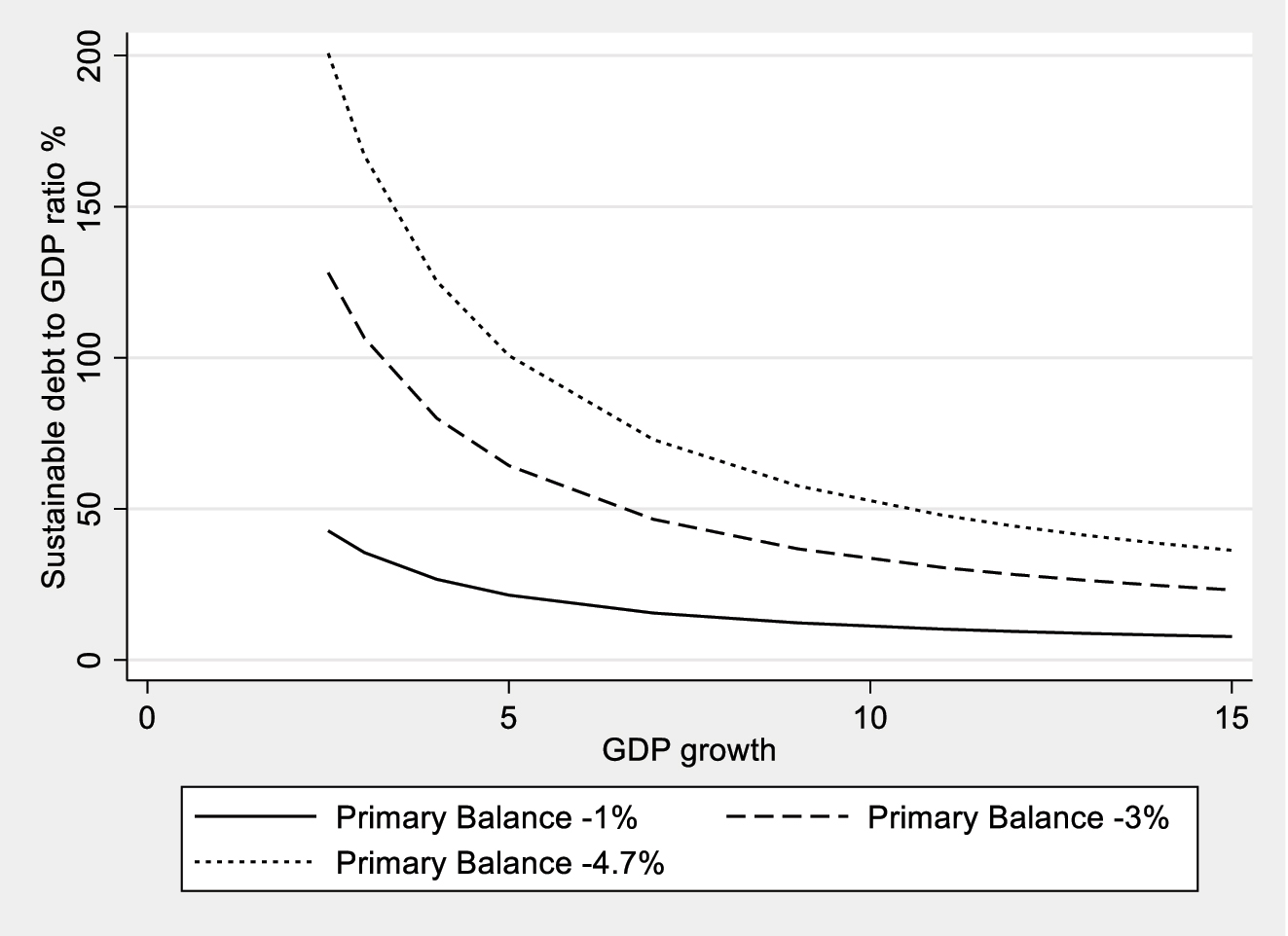
Debt burden and real GDP growth for alternative levels of budget deficit.
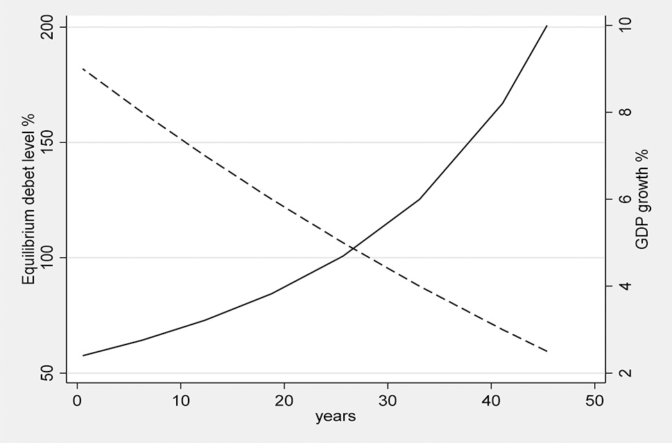
Even when debt is sustainable, it would take years to clear arrears with sluggish growth.
3.2 Climate Change and the Debt Burden in Africa
Using the above insights and results from Table 1, it is possible to assess the potential impact of climate-induced shocks on debt trajectories in Africa. As noted, a rise in temperature beyond 30 °C could cost Africa 2 percentage point decline in real GDP growth. Similarly, the elasticity of budget deficit to real GDP growth computed from our data is around 0.3 percentage points as a share of GDP. Figure 7 presents robust and positive correlation between real GDP growth and fiscal deficit in Africa showing that growth losses would worsen fiscal deficit and vice versa.
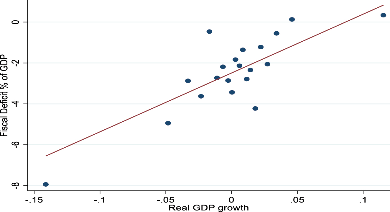
Correlation between fiscal deficit and real GDP growth in Africa. The scatter diagram controls for political stability and institutional quality.
Putting these facts together it is possible to evaluate the maximum debt burden beyond which a country could become insolvent. To give the order of magnitude, first we evaluate the debt-carrying capacity of African economy based on long-term growth achieved in the “good times”, which stood around 5 % (2000–2013). The average budget deficit (primary) during this period was around 2.8 % of GDP. Noting that most African countries benefited for many years from concessional loans, real interest rate varied between 1% and 2%. Taking the lower bound of 1 % real interest rate, the implied ‘optimal’ debt-burden would be around 73 % of GDP. Now taking the shift in real GDP growth caused by climate change induced shocks and the budget deficit together, the debt-GDP ratio would increase to 175 % of GDP. Such a scenario suggest how unattended climate change risk could easily increase the debt burden and undermine fiscal space badly needed for taking measures to contain greenhouse gas emissions.
4 Transition to a Low-Carbon Economy: Cost and Benefits
This section analyses what the transition to a low-carbon pathway means for Africa. The discussion starts with an analysis of historical trends of energy use and sources to assess how far Africa has been adjusting its sources of energy over the past decade and the potential for renewable energy. Next, we discuss the opportunities and challenges associated with the impending trading on a global carbon market. Following that we discuss what the Just Energy Transition means for Africa, including an assessment of the costs of transitioning to low-carbon pathways.
4.1 Trends in Emissions and Energy Production
Figure 8 shows that Africa emissions are relatively low compared to other countries and regions. For example, in 2019 emissions for the largest emitter on the continent, South Africa, was 226 MtCO2 compared to 5,256 MtCO2 for the US and 10,490 MtCO2 for China. Africa’s emissions are low due to the lower level of economic activity compared to other regions and because most of the population lacks access to electricity and clean cooking solutions.
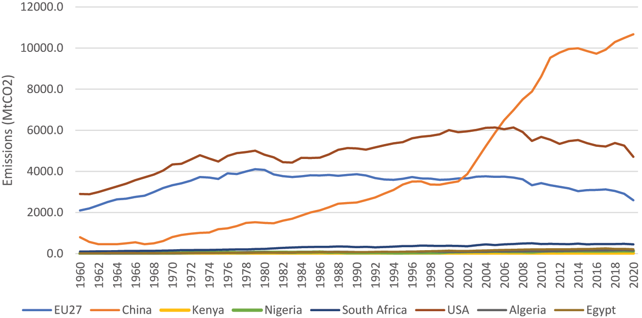
Carbon dioxide emissions for selected countries, 1960–2020. Source: Andrew and Peters (2021).
Currently, Africa produces only 4 % of global GDP and about 6 % of global energy. However, Africa’s population could grow significantly in the future and, by 2100, more than a quarter of the world’s population could be living on the continent. This could put upward pressure on global emissions depending on the energy transition pathways that countries choose. However, African countries have signalled their intensions to contribute to lowering global emissions. Following the 2015 United Nations Climate Change Conference, COP23, in Paris, all 54 African countries have signed the Paris Agreement and submitted ambitious Nationally Determined Contributions (NDCs), while most of them have ratified their NDCs.
Figure 9 shows trends in energy production by source for Africa in the period 2010 to 2019 for natural gas, crude oil, hydro, solar PV, and wind. The data show a meteoric rise in the production of energy from renewables such as solar and wind. Over the past decade, the take up of solar PV has increased by 20-fold while that of wind energy has increased by nearly seven-fold. On the other hand, production of crude oil fell by 19 % in this period. These results show that, to some extent, African countries have gone cleaner. And judging from their NDCs, many of them have shown ambitions to embrace a low-carbon economy. We discuss below that the transition may not be as easy and that challenges will have to be addressed.
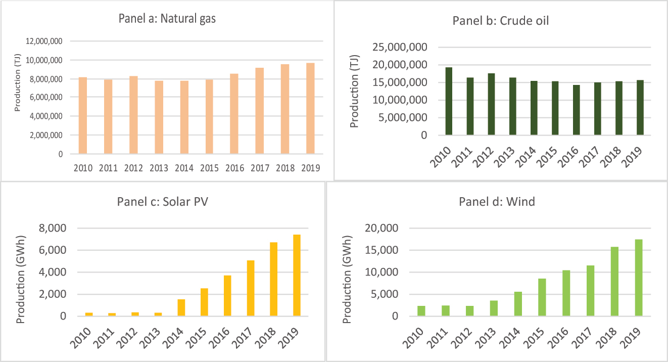
Africa’s energy production by source, 2010–19. Source: IEA (2021).
Africa has abundant supplies of renewable energy that could be leveraged in the global carbon market. According to the International Renewable Energy Agency, Africa’s total energy potential for CSP, PV, and wind energy is about 1,585 Petawatt hours (PWh) per year, broken down as follows: CSP, 479 PWh; PV, 640 PWh; and wind, 460 PWh (see Figure 8). For both CSP and PV, East Africa has the highest potential (176 PWh for CSP and 220 PWh for PV), followed by Southern Africa (150 PWh for CSP and 160 PWh for PV). North Africa has potential of about 100 PWh for both CSP and PV. West Africa is endowed with good PV potential (104 PWh) but limited CSP potential (30 PWh) because of less direct irradiation and higher “solar fluctuations” (IRENA 2014). Central Africa has relatively low potential for either CSP or PV compared with the other regions (Figure 10).
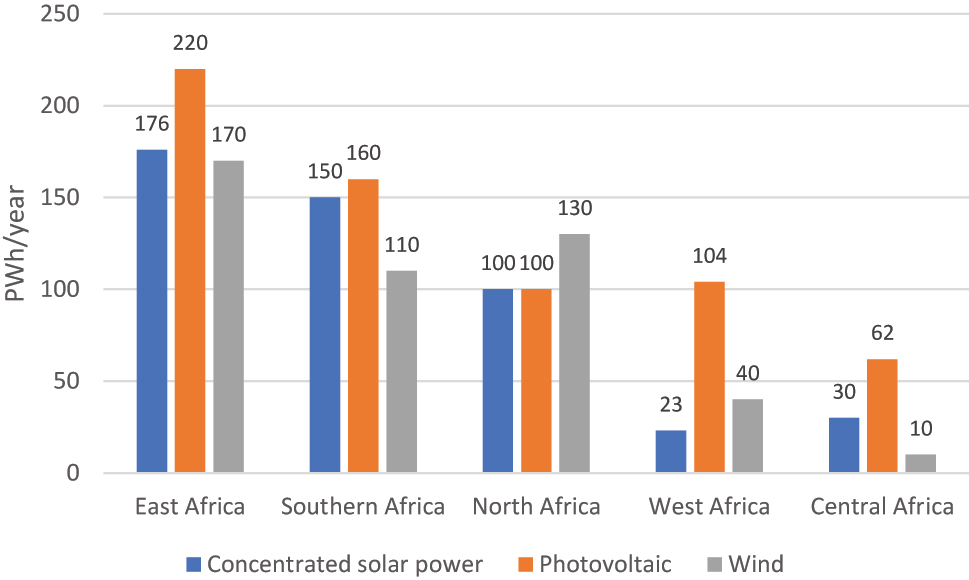
Africa’s renewable energy resources, 2013. Source: IRENA (2014).
4.2 Carbon Trading
Africa currently accounts for around 2 % of trading in the international carbon market. South Africa and North Africa get the bulk of Clean Development Mechanism (CDM) funds under the Kyoto Protocol. In June 2021, Gabon became the first African country to receive climate finance of up to $150 million over 10 years. During COP26, countries reached agreement on Article 6 of the 2015 Paris Agreement to pave the way for the establishment of a regulated international carbon market. It is likely that modalities and timelines will be announced at COP27. Africa needs to be ready to be a significant player in this global market given its massive carbon stocks. Many countries around the world currently have energy efficiency and renewable policies and over 50 national or sub-national governments have implemented carbon pricing (World Bank 2019) in the form of carbon taxation or emissions trading schemes (ETS). A few African countries have shown interest in using carbon pricing to meet their NDCs. South Africa was the first to introduce a carbon tax in 2019 and other countries such as Kenya, Ethiopia, Egypt, and Côte d’Ivoire are considering schemes involving an ETS or carbon tax.
The main challenges of implementing carbon pricing (whether ETS or carbon tax) schemes in Africa include the fact that they can be administratively burdensome and subject to their design, can require a complex architecture of institutions. This is particularly the case for the ETS, making carbon tax systems relatively preferable from an implementation perspective. Such systems also require enforcement capacity, again something that is a challenge for several African countries. At a minimum, and subject to the design of the carbon pricing instrument, countries would most likely require a comprehensive monitoring/estimation and reporting framework for the emissions or inputs/outputs on which the price is imposed, a system that many African countries are still in the process of developing. Furthermore, although these schemes have the potential to generate revenue, they can also have regressive effects, particularly on low-income households, if not well designed.
4.3 The Just Energy Transition
The idea of a Just Transition is premised on the fact that the shift to low- or zero- carbon economies must be a shared global responsibility with the benefits being distributed fairly and that some communities should not be worse off as a result. In the case of SSA, most of the population do not have access to electricity and clean cooking solutions and must rely on biomass for household thermal energy. Going into COP27, Africa will make a strong case for natural gas to be part of its Just Energy Transition systems. This is because, to improve energy access, Africa cannot rely entirely on renewables due to their intermittency. Africa needs to combine renewables with natural gas to assure stability and energy security, as well as to improve access and affordability. Given Africa’s energy profile shown in Figure 6 above, even if Africa triples the use of gas-to-power, it will contribute less than 1 % to global carbon emissions.
Another aspect of the Just Energy Transition is the cost involved. Estimates of adaptation and mitigation costs in the NDCs are just the direct costs. They do not include the ‘adjustment’ or indirect costs of transitioning to low carbon pathways. For example, they do not include the costs of job losses in carbon-intensive sectors and possible stranded assets. A recent study by McKinsey estimates the cost of the net zero transition to be equivalent to 6.8 % of global GDP in 2021, rising to 8.8 % from 2026 to 2030 (McKinsey Global Institute 2022). It also estimates that 200 million jobs could be created, but 185 million direct and indirect jobs could be lost. In the case of Africa, countries would need to invest 1.5 times or more compared to advanced economies as a share of GDP today to support economic development and build low-carbon infrastructure to enable a shift to net-zero greenhouse gas emissions. In developing regions, expenditures on energy and land would form a substantially larger share of national GDP: about 10 % in Africa, India and some other Asian countries, and Latin America.
To get some further indication of the indirect costs of the low-carbon energy transition for African countries, we estimated the macroeconomic and sectoral impacts of using carbon pricing as an instrument to achieve the NDCs. We used South Africa, Nigeria, and Egypt, who are among the high African emitters, as examples. For this analysis, we used the GTAP-E model developed by Burniaux and Truong (2002) and revised by McDougall and Golub (2007), together with the GTAP-E Database Version 10.
South Africa’s carbon tax is envisioned to be a fuel input tax, based on the carbon content of the fuel used, and will cover all stationary direct greenhouse gas emissions from both fuel combustion and non-energy industrial process emissions, amounting to approximately 80 % of total emissions. The tax was implemented on 1st June 2019 at a rate of R120 (US$7.46) per tonne CO2e. On January 1, 2022, the finance minister announced an increase to R144 (US$9) per tonne CO2e. To uphold South Africa’s NDCs, the rate will increase each year by at least US$1 until it reaches US$20. Since Nigeria and Egypt have not yet announced carbon pricing policies, we applied a tax of US$9 as South Africa has just done. We also run another simulation with a higher tax of US$$20 per tonne CO2e to investigate the effects of a further escalation of the tax.
Table 3 shows that the carbon tax leads a contraction in the GDP of Nigeria (−0.10 %) and South Africa (−0.58 %) but has a small positive effect (0.03 %) on that of Egypt.
Macroeconomic impacts of a US$9 per tonne carbon tax.
| Variable | Nigeria | South Africa | Egypt |
|---|---|---|---|
| GDP (% change) | −0.10 | −0.58 | 0.03 |
| Private consumption (% change) | −0.01 | −0.26 | −0.04 |
| Exports (% change) | 0.18 | 0.71 | 0.36 |
| Imports (% change) | −0.26 | −1.78 | −0.14 |
| Terms of trade (% change) | −0.04 | −0.10 | −0.05 |
| Trade balance (US$ mil.) | 357.90 | 2,888.28 | 308.15 |
| CO2 emissions (% change) | −2.78 | −13.21 | −6.79 |
| Welfare (based on EV, US$ mil.) | −44.06 | −805.83 | −125.11 |
-
Source: GTAP-E model simulations.
The tax leads to rises in the prices of energy-intensive products and services such coal, gas, and electricity (see Table 5), which causes private consumption expenditure to decline in all three countries. This in turn leads to declines in real income (measured by equivalent variation) of US$44 million, US$805 million, and US$125 million, respectively, for Nigeria, South Africa, and Egypt.
On the external side, Table 4 shows that exports increase faster than imports, resulting in trade balances of US$357 million, US$2,888 million, and US$305 million, respectively, for Nigeria, South Africa, and Egypt. The results indicate that CO2 emissions fall by 13 % in South Africa, by 7 % in Egypt, and by 3 % in Nigeria (see Table 3), which suggest that carbon pricing could be an effective means of reducing emissions to meet the NDCs.
Sectoral impacts of a US$9 per tonne carbon tax (% change from base level).
| Sector | Nigeria | South Africa | Egypt |
|---|---|---|---|
| Agriculture | 0.01 | 0.10 | 0.06 |
| Coal | −8.38 | −6.20 | −9.25 |
| Oil | 0.18 | 0.53 | 0.06 |
| Gas | −0.51 | −4.11 | −9.28 |
| Oil products | −3.38 | −2.65 | −1.05 |
| Electricity | −2.72 | −12.78 | −2.59 |
| Energy-intensive industries | −1.83 | −1.32 | −0.73 |
| Other industries & services | −0.06 | −0.10 | 0.01 |
-
Source: GTAP-E model simulations.
Table 4 shows that the tax results in improvements in the outputs of the agriculture and oil sectors, which result in declines in their prices as shown in Table 5. On the other hand, there are contractions in the outputs of coal, gas, and energy-intensive industries and services.
Impacts of a US$9 carbon tax on product prices (% change from base level).
| Product | Nigeria | South Africa | Egypt |
|---|---|---|---|
| Agriculture | −0.17 | −0.20 | −0.09 |
| Coal | 14.22 | 30.24 | 24.56 |
| Oil | −0.05 | −0.67 | −0.20 |
| Gas | 10.69 | 5.54 | 20.91 |
| Oil products | 4.09 | 3.66 | 4.04 |
| Electricity | 4.63 | 13.37 | 5.03 |
| Energy-intensive industries | 0.55 | 0.33 | 0.30 |
| Other industries & services | −0.10 | −0.70 | −0.10 |
-
Source: GTAP-E model simulations.
The results for a carbon tax of US$20 per tonne are shown in Table 6. It can be seen that whereas there is not much change in Egypt’s GDP, those of Nigeria and South Africa decline by 0.25 % and 1.29 %, respectively. Private consumption declines by similar amounts in Nigeria and South Africa, while it increases slightly by 0.04 % in Egypt. As was the case in the previous scenario, a carbon tax is advantageous for the external sector. A carbon tax of US$20 per tonne carbon tax leads to an increase in exports and decline in imports, resulting in a doubling of the trade balance in all three countries. The US$20 carbon tax also results in faster progress towards achieving the NDCs as CO2 emissions decline by about 24 %, 13 % and 6 %, respectively, in South Africa, Nigeria, and Egypt. However, the US$20 carbon tax intensifies the adverse welfare impacts on households due to the rapid rise in the price of utilities and products of carbon-intensive industries. In this scenario, welfare based on equivalent variation declines by US$2,107 million in South Africa, US$385 million in Egypt and by US$131 million in Nigeria.
Macroeconomic impacts of a US$20 per tonne carbon tax.
| Variable | Nigeria | South Africa | Egypt |
|---|---|---|---|
| GDP (% change) | −0.25 | −1.29 | 0.04 |
| Private consumption (% change) | −0.27 | −1.33 | 0.04 |
| Exports (% change) | 0.43 | 1.47 | 0.78 |
| Imports (% change) | −0.67 | −3.66 | −0.3 |
| Terms of trade (% change) | −0.11 | −0.21 | −0.12 |
| Trade balance (US$ mil.) | 873.73 | 5,941.62 | 661.73 |
| CO2 emissions (% change) | −6.39 | −24.03 | −13.45 |
| Welfare (based on EV, US$ mil.) | −130.88 | −2,107.45 | −384.57 |
-
Source: GTAP-E model simulations.
The foregoing results have two key implications for the design of carbon pricing schemes in Africa. First, the fall in the output of energy-intensive sectors will lead to job losses (not measured here). Therefore, there would be a need for retraining of workers for employment in other sectors. Second, the increased price of electricity and energy-intensive goods will have a greater impact on low-income households. The share of the income of low-income households spent on electricity and energy-intensive goods would be greater (given that electricity consumption is relatively price inelastic), leading to much more adverse effects on their welfare. Therefore, part of the revenues generated from the carbon tax could be used to address the negative impacts on these groups.
5 Conclusions and Policy Implications
5.1 Conclusions
Although Africa contributes less than 3 % of total global GHGs, it suffers the most from climate change shocks. Our preliminary findings suggest that Africa’s real GDP growth could decline by about 2 percentage points for a temperature change above 1.8 °C. Projections by the Intergovernmental Panel on Climate Change (IPCC) indicate that the frequency and intensity of climate-related events such as natural disasters (i.e. droughts and floods) will increase in the coming decades. In this paper, we have shown that this could exacerbate political instability and conflict. These shocks combined could have a direct effect on government fiscal position and subsequently on sustainability of debt. For example, a 1 % decline in real GDP growth could worsen the budget deficit by 0.3 percentage points, and this could increase the debt-burden by 2.4 times.
All African countries have signed the Paris Agreement and have submitted their NDCs that contain targets for emissions reductions. Our modelling results indicate that carbon pricing could be an effective way of meeting the NDCs. However, carbon pricing (e.g. a carbon tax) would have negative impacts on energy-intensive industries and increase the prices of the goods and services they provide. There will also be job losses in these industries. The combined effect of these impacts could be reduction in GDP growth and real incomes. From the modelling results, we infer that carbon pricing can have regressive effects, particularly on low-income households, if not well designed.
5.2 Policy Implications
The study results have several implications for policy makers. First, Africa has significant stocks of renewable natural resources that could be leveraged in a future global carbon market to speed up economic transformation and improve the well-being of the people. However, significant foreign investment and technology is required to make this a reality. To attract the needed investment, African governments should develop a stable regulatory and policy environment and establish competitive pricing to promote mini-grid solutions and standalone systems.
Second, participation in international carbon markets and offset schemes (e.g. REDD+, CDM) requires a credible system for measuring, reporting, and verifying emissions. However, many African countries have been unable to accurately measure and report the carbon sequestered in their forests. At COP27, Africa needs to push for more capacity building and technical assistance. Furthermore, improvements need to be made in forest governance and land tenure. In general, forest governance in Africa suffers from poor institutional capacity and performance and insecure or weak land and forest tenure by local communities. Less than 2 % of Africa’s forests are estimated to be legally owned or designated for use by local communities (Allen 2011). Land tenure reforms are urgently needed to enable indigenous and local communities to claim property rights in forest land to benefit from payments from carbon trading and offset schemes.
Third, in the transition to low-carbon pathways, the world would need African resources. Although accounting for a small proportion of current global resources, Africa has a significant proportion of untapped mineral reserves: 30 % of bauxite, 60 % of manganese, 75 % of phosphates, 85 % of platinum, 30 % of titanium and 60 % of cobalt. There is therefore the need to ensure that sustainable techniques are used, and fair employment practices are enforced.
Finally, several countries such as Burkina Faso, Côte d’Ivoire, Nigeria, Rwanda, and Senegal have expressed an interest in advancing carbon pricing at a domestic level. There is also interest in carbon pricing at the regional level. For example, two new regional groups, the West African Alliance on Carbon Markets and Climate Finance (WAA), and the East African Alliance on Carbon Markets and Climate Finance (EAA), have expressed an interest in regional carbon pricing initiatives. This could lead to the implementation of a regional carbon tax or ETS. However, this would require significant regional collaboration and leadership. For example, regional collaboration would be required to amend and enhance legal frameworks to facilitate implementation and administration of the scheme. There would also be the need to build capacity and expertise to assess carbon pricing options and implement the mechanisms.
Funding source: African Economic Research Consortium
Award Identifier / Grant number: AERC/Boston/002/2003
References
Abiad, Abdul, and D. Ostry. 2005. “Primary Surpluses and Sustainable Debt Levels in Emerging Market Countries.” IMF Working Papers. https://doi.org/10.5089/9781451975703.003.Search in Google Scholar
Abidoye, Babatunde O., and Ayodele F. Odusola. 2015. “Climate Change and Economic Growth in Africa: An Econometric Analysis.” Journal of African Economies 24 (2): 277–301. https://doi.org/10.1093/jae/eju033.Search in Google Scholar
Adesina, A. A. 2021. Leaders’ Summit on Climate. Available from: https://www.afdb.org/en/news-and-events/press-releases/leaders-summit-climate-african-development-bank-president-says-continent-ground-zero-crisis-major-economies-boost-climate-targets-43272.Search in Google Scholar
African Development Bank. 2019. The State and Dynamics of Debt in Africa. Abidjan: Mimeo.Search in Google Scholar
Allen, D. W. 2011. “Legalising Land Rights Local Practices, State Responses, and Tenure Security in Africa, Asia and Latin America.” Agricultural History 85 (1): 119–20.Search in Google Scholar
Andrew, Robbie, and Peters, Glen. 2021. “The Global Carbon Project’s Fossil CO2 Emissions Dataset.” figshare. https://doi.org/10.6084/m9.figshare.16729084.v1.Search in Google Scholar
Baarsch, L., Jessie R. Granadillos, William Hare, Maria Knaus, Mario Krapp, Michiel Schaeffer, and Hermann Lotze-Campen. 2020. “The Impact of Climate Change on Incomes and Convergence in Africa.” World Development 126.10.1016/j.worlddev.2019.104699Search in Google Scholar
Barro, R. J. 1991. “Economic Growth in a Cross Section of Countries.” Quarterly Journal of Economics 106 (2): 407–43. https://doi.org/10.2307/2937943.Search in Google Scholar
Barro, Robert. 1996. “Determinants of Economic Growth: A Cross-Country Empirical Study.” Working Paper 5698. Cambridge: NBER. https://doi.org/10.3386/w5698.Search in Google Scholar
Burniaux, J. M., and T. P. Truong. 2002. “GTAP-E: An Energy-Environmental Version of the GTAP Model.” In GTAP Technical Paper No. 18, Center for Global Trade Analysis. Department of Agricultural Economics. West Lafayette: Purdue University.10.21642/GTAP.TP16Search in Google Scholar
Felbermayr, Gabriel, and Jasmin Gröschl. 2014. “Naturally Negative: The Growth Effects of Natural Disasters.” Journal of Development Economics 111 (C): 92–106. https://doi.org/10.1016/j.jdeveco.2014.07.004.Search in Google Scholar
International Energy Agency, IEA. 2021. Data and Statistics. Available from: https://www.iea.org/data-and-statistics/datatables?country=WEOAFRICA&energy=Natural%20gas&year=2019.Search in Google Scholar
IRENA (International Renewable Energy Agency). 2014. Estimating the Renewable Energy Potential in Africa: A GIS-Based Approach. Abu Dhabi: IRENA. Available from: http://www.irena.org/DocumentDownloads/Publications/IRENA_Africa_Resource_Potential_Aug2014.pdf.Search in Google Scholar
Jarmuzek, Mariusz, and Yanliang Miao. 2013. A Primer on Estimating Indicative Public Debt Thresholds. IMF Working Papers.Search in Google Scholar
McDougall, R., and A. Golub. 2007. GTAP-e: A Revised Energy-Environmental Version of the GTAP Model. GTAP Research Memorandum, 15, Center for Global Trade Analysis. Department of Agricultural Economics. West Lafayette: Purdue University.Search in Google Scholar
McKinsey Global Institute. 2022. The Net-Zero Transition: What It Would Cost, What It Would Bring. Available from: https://www.mckinsey.com/business-functions/sustainability/our-insights/the-net-zero-transition-what-it-would-cost-what-it-could-bring.Search in Google Scholar
Rankin, Neil, and Barbara Roffia. 2003. “Maximum Sustainable Government Debt in the Overlapping Generations Model.” The Manchester School 71 (3): 217–41. https://doi.org/10.1111/1467-9957.00344.Search in Google Scholar
World Bank. 2019. State and Trends of Carbon Pricing 2019. Washington, DC. https://doi.org/10.1596/978-1-4648-1435-8.Search in Google Scholar
© 2024 Walter de Gruyter GmbH, Berlin/Boston
Articles in the same Issue
- Frontmatter
- Policy Analysis
- An Analysis of the IMF’s International Carbon Price Floor
- India’s Energy and Fiscal Transition
- Macroeconomic and Fiscal Consequences of Climate Change in Latin America and the Caribbean
- Symposia_Articles
- Sovereign Debt and Climate Change in Argentina – The Catalytic Role of the IMF
- Climate Change Risks and Consequences on Growth and Debt-Sustainability in Africa
- Policy Analysis
- Gaps and Fiscal Adjustment for Debt Stability in Climate-Vulnerable Developing Countries: How Large and by How Much?