An Alternative Approach to Frequency of Patent Technology Codes: The Case of Renewable Energy Generation
-
Diana Terrazas-Santamaria
 ,
Saul Mendoza-Palacios
,
Saul Mendoza-Palacios

Abstract
This article proposes a methodology to identify technological transitions (TTs) by systematically using the total variation distance (TVD) metric. We use a database of renewable energy generation (REG) patents to exemplify the usefulness of TVD to uncover moments where a “big change” in REG technology happened. To do this, we compare the observed frequency distribution of technology codes of REG patents filed between 1973 and 2015 in the US, spread across seven categories (e.g., wind and tidal). We identify two crucial TTs, one at the beginning of the 1980s and another in the late 1990s and early 2000s. In this manner, we reconcile qualitative evidence that registers major REG changes with a quantitative measure that reflects them. Policy evaluations or causality analyses often rely on identifying TTs accurately; therefore, this approach is not constrained to the REG technology or TTs but helps reveal such transition moments in a database whose characteristics are suitable for the use of TVD.
1 Introduction
Technological changes are one of the leading forces to explain economic growth and development. They happen continuously, and at some moments during a time span, they are especially relevant since these changes occur abruptly. As Perez-Molina and Loizides (2021) state different agents, such as researchers or private firms, continuously look for tools to understand a specific technology’s evolution and pinpoint moments of particular interest within it. In this context, we are interested in identifying technological transitions (TTs), which we refer to as those moments when the technology in a particular field exhibits a notable change.
TTs are complex phenomena with effects on innovative processes, organization of production factors, products, and new ideas. Not all these innovations can be legally protected, or owners may decide not to do so even if they can. Despite this limitation, patents serve as a proxy for successful innovation processes and allow us to use analytical approaches to study the complex dynamics behind them (Alkemade et al., 2015). Patent documents have been widely used in the academic literature since they provide valuable information about the state of a given technology at a given time. Specifically, patent classification has been a primordial instrument for creating a useful taxonomy that can be used by those interested in protecting and analyzing intellectual property (e.g., Meguro & Osabe, 2019; Ruijie et al., 2021).
This article proposes a methodology to systematically identify TTs in a particular technological field using the distance between probability distributions among the technology codes in that field. We characterize a technological state as the probabilistic empirical density distribution over the technological patent categories at a given time, using the Cooperative Patent Classification (CPC). Consequently, we approach technological change by measuring the distance between these distributions.
As discussed in Frenken et al. (2014), we conceive a TT as a tipping point in which the dominant technological state changes to an alternative one within a given system. Therefore, we claim that a disruptive change in the distribution of categories can be used as a signal of a TT. Hence, the interest of this article is not to explain the drivers behind a TT or mathematically model them, but to offer an alternative methodology for a systematic exploratory analysis of the identification of TTs.
To the best of our knowledge, the methodology of intertemporally measuring the distance between distributions within a given technology has not been used to identify historical moments where a notable technological change may have occurred. Since technological change is a continuous phenomenon, we focus on “big” changes. We measure it with the total variation distance (TVD) metric based on its properties and explain why we use local maxima to identify TTs (Section 3).
Our proposed methodology is easily executable and straightforward to interpret since it only uses the relative frequency of each category at a given time as an input, and the TVD’s values range from 0 to 2. Thus, it is particularly valuable for exploratory analysis, providing a visualization tool to identify TTs. We use patent data from the renewable energy generation (REG), which shows suitable data characteristics (Section 2), and we identify two TTs consistent with the REG historical evidence. To show the validity of our methodology, we perform a chi-square test of independence, and the results are in line with the TVD results.
This article is organized as follows. Section 2 compares our methodology to the existing literature on the identification of TTs. Section 3 introduces the TVD and its properties and explains its calculation. In Section 4, we present the REG case and data set, for which we calculate the TVD under different specifications and discuss the interpretation of two identified moments of TT. We conclude in Section 5.
2 Related Literature
TVD is a probabilistic measure to quantify the difference between two probability density functions (pdfs). A distance is a quantitative measure of how far apart two objects are, and measuring the distance between histograms has proven paramount in various areas to perform pattern recognition (Cha & Srihari, 2002; Kurtz et al., 2013; Strelkov, 2008). If we consider a nominal histogram, which is our case, it represents the distribution of quantified labeled values (categories) where each bin contains the proportion of a category out of all categories, and their ordering is not important (shuffling invariance property)[1] (Sung-Hyuk, 2007; Kurtz et al., 2013).
Thus, at a given period, the histogram that portrays the relative frequency of patents distributed in different categories within a given technology intrinsically provides information on what the innovative interests are at that time, or what we refer to as the technological state. Consequently, measuring the probabilistic distance between two nominal histograms at two points in time provides valuable information on how close or apart the inventive efforts were.
As Strelkov (2008) points out, humans compare multiple histograms relatively slowly, and a comparison algorithm is preferable; however, for such an algorithm to be reliable, it needs to reach conclusions close to those reached using distinct methods. Cha and Srihari (2002) explain that, in the probabilistic distance approach, a histogram provides the empirical estimate of the pdf and compares corresponding and non-corresponding bins.[2]
Our TVD approach measures the distance between two empirical distributions. Thus, if, at a given period, this distance is considerably greater than the historical ones, we can contemplate the existence of an abrupt change in the technology at that point, or a TT. In this manner, we contribute to the TTs’ literature using patents by proposing a methodology used in several disciplines, but to the best of our knowledge, which had not previously been used in this context, or intertemporally. Examples of TVD usefulness are found in genomics (Garcia & Pinho, 2011), criminology (Carte et al., 2020), epidemic models (Ball & Donnelly, 1995), biology of sleep (Barger et al., 2019), and, more generally, time series with similar oscillations (Euán et al., 2018).
Since a patent is classified in all the relevant technology codes where the novelty fits (Lobo & Strumsky, 2019), its classification codes are proxies of its different technological components (Perez-Molina & Loizides, 2021), and the historical information of how these codes evolved within a technology can uncover trends or statistically identify when innovative efforts shifted. The increased availability of patent data since the 1970s has served to study technological evolution (Martino, 1971). We extend such study to the evolution of the distribution of a technological field over the exogenously determined codes using the distance over their distribution.
Conventional TT measurements include indicators based on patent filings, application dates, or grant counts, which have been recently combined with text analysis (e.g., Guderian, 2019; Lacasa et al., 2003). We acknowledge that the number of technology codes driven by patents has been used to capture changes in technological capabilities (e.g., Lobo et al., 2012) or to assess the growth of a particular subgroup of patents with respect to the total (e.g., Angelucci et al., 2012; Bae & Kim, 2017). However, instead of analyzing technology as a set that evolves due to the relative change of its components, as we do, these methodologies have focused primarily on isolated fields within a technology.
3 Methodology
Next, we explain the TVD, its properties, and the reasons it is preferable for our case rather than other probabilistic distances. The TVD is a probabilistic measure to quantify the difference between two pdfs; it measures their similarity.
If the sample space is discrete and categorical, as in our REG case, the TVD measures the difference of histograms by categories. Let
In probability theory, there are different ways to measure the distance between two probability distributions. A few of these are TVD, Hellinger distance, Kullback-Leibler divergence, Wasserstein distance, Prokhorov distance, among others (see Massart, 2007, for further discussion). The first two metrize strong topology, and the last two metrize weak convergence; Kullback-Leibler divergence is not a distance, but its proximity implies strong and weak convergence. Also, Lin et al. (2021) use the Kullback–Leibler divergence to identify technology life cycles.
We select TVD because:
It is not sentient to the distance
It has properties similar to a norm in vector spaces. In particular, it is homogeneous. That is, the distance between the average of two distributions and one of the two is proportional to the distance between the two initial distributions, unlike weak topology metrics.
Its calculation is more straightforward compared to other strong topology metrics, such as the Hellinger distance, and its interpretation is more intuitive.
Since it is a distance, it allows us to measure the difference between several probability distributions, in contrast to the Kullback-Leibler divergence.[3]
It can be calculated for probability distributions for which the probability of an event is 0, in contrast to the Jensen–Shannon divergence.
It is sensitive to changes in the distribution concerning all the categories, as opposed to the separation distance.
Due to the aforementioned reasons, we find TVD a suitable measure for qualitative categories where the order is not relevant, as is the case with patent technology codes, and it allows for a pairwise comparison between different distributions without having to have the same base.
3.1 TTs’ Identification Methodology
If equation (1) is strictly positive, then we have a technological state (or technological change) change between periods
While a distance only allows for pairwise comparisons for a particular order of periods
TVD is invariant to the number of observations at each period since it depends on the relative distribution. However, the number of observations in a distribution affects its variability. To avoid misguided interpretations related to a change of the TVD that may respond to the total number of observations, we consider two types of periods:
Natural periods, in which each distribution includes the observations of one or several calendar years.
Periods with the same number of observations (PSNO), in which we partition the data into consecutive subsets, each with the same number of observations, making a further breakdown by month and day.
Note that TVD is not sensitive to category reordering. TVD may vary to a certain degree in the absence of a TT; such variation depends on the nature of the technological field and moment, as well as the total number of observations in each period. Therefore, in absolute terms, we cannot claim any particular TVD level to be indicative of a TT. Instead, we focus on local maxima specific to the technological field under study, which show a greater distance both directions in time.
The application of the TVD as an identification strategy of TTs requires the adequate identification of technological fields, which contain emergent technological innovations. A narrow field selection could exclude potential emergent technological innovations. In our example, the sources that REG use as primary (e.g., wind, water, or sun) have not changed in at least the last century, and we can reasonably argue that those categories are fixed in our period of analysis. Suppose a new category appears at a particular moment in time. In that circumstance, we can either reorganize the previous observations according to the new categorization, assume that none of the previous (posterior) observations belong to the newly created (eliminated) category, or introduce an interpolation.
4 The REG Case
4.1 CPC
Much has been discussed about how patent offices prepare to tackle a sudden increase in patents due to the rapid development of emerging technologies. For instance, evidence suggests that public and private investment in R&D in nanotechnology led to a significant rise in related patent applications (Absalom et al., 2006; Angelucci et al., 2012). Absalom et al. (2006) mention that the European Patent Office (EPO) developed a new taxonomy in the early stages of nanotechnology R&D to ensure technical expertise within examiners and legal certainty to innovators. In this way, patents contain information about the birth and development of technologies.
One difficulty of reliably identifying whether a TT has occurred is to ensure consistent patent classifications throughout the period of study (Lacasa et al., 2003). On October 25, 2010, the EPO and the United States Patent and Trademark Office (USPTO) announced the CPC as a joint effort aimed at establishing a harmonized classification system for patent documents; the CPC is based on the International Patent Classification system, managed by the World Intellectual Property Organization.[4]
The CPC is divided into nine sections (A-H and Y), where each section is divided into classes, subclasses, groups, and subgroups, containing approximately 250,000 classification entries.[5] In our illustrative case, we use patents with at least one Current CPC Class within the subgroups of the Y02E 10 group of “Energy generation through renewable energy sources”[6] (Section 4).
One important peculiarity of the Y-section is that the allocation of new patent applications to the relevant technology code(s) is done automatically by search strategies without affecting existing classifications outside it; thus, classifiers’ intervention is constrained to developing and updating those strategies (EPO & USPTO, 2015). Furthermore, within the Y-section results, there has been a dedicated effort to reclassify all applicable patents, retroactively, with meticulous work and continuous tagging by the various patent offices, ensuring that the Y02E 10 subgroups contain only REG-related patents.
In this manner, we take advantage of the categorical property of the subgroups within the Y02E 10 group of “Energy generation through renewable energy sources” from the Current CPC Class, which contains only REG-related patents. Thus, each of the seven subgroups of the Y02E 10 group, also called categories, belongs to a different renewable energy source (e.g., wind or from the sea). We use categories that are known beforehand, where patents are sorted into seven separate categories. All patents classified under the “Wind” category are useful to generate energy using the wind but are sufficiently different from those “From the sea.”[7]
Climate change mitigation technologies (CCMTs) involve several areas of knowledge. Thus, technologies using the existing alternative patent classifications can lead to an incomplete retrieval of documents. As stated by the EPO, “Y02 is a tagging scheme that enables documents relating to sustainable technologies to be retrieved quickly and accurately across classification categories.”[8]
4.2 The Data Set
We illustrate the implementation of TDV using public patent data provided by the USPTO. In particular, we consider patents with at least one Current CPC Class[9] within the Y02E 10 group of “Energy generation through renewable energy sources.” The Y02 class aims to identify CCMTs as stated in the Kyoto Agreement (Angelucci et al., 2012), which contains the Y02E subclass, “Reduction of greenhouse gas emissions, related to energy generation, transmissions or distribution.”
We searched all patents within each subgroup of Y02E 10 group (one-dot level, two-dot level, and three-dot level).[10] Each subgroup contains materials, systems, or structures used in energy generation depending on the renewable source.[11] For instance, in photovoltaic (PV) energy, the one-dot level is Y02E 10/50 “PV energy,” a two-dot level is Y02E 10/54 “Material technologies,” and a three-dot level is Y02E 10/545 “Microcrystalline silicon PV cells.”
Our database consists of 39,236 patents filed from 1973 to 2015. Although there is updated information on patent applications, we decided to exclude patents filed from 2016 onward from the analysis to avoid false TTs due to unobserved recent patent applications. This phenomenon exists because in Article 1122 of the Manual of Patent Examining Procedure, the USPTO allows for the possibility of requesting an application to be non-publishable until its acceptance, so we may not have been able to publicly observe the accurate quantity of recent applications. Considering patents granted up to January 2020,[12] the mean lag between the issuance and their filing date is 2.9 years, with a standard deviation of 1.5 years. Therefore, we decided to exclude patents corresponding to the period close to the mean lag plus one standard deviation.[13] Note that the mean lag in our database is close to 2.4 years obtained by Popp et al. (2004).
A patent can have more than one Current CPC Class, but we analyzed only those patents recorded with at least one of the REG categories (Table 1). When all subgroups within REG belong to only one subgroup, we assigned a patent to that category. However, when the subgroups belong to two categories, these patents appear in two categories; the same principle applies to patents with three or more subgroups.
Current CPC classes considered in each REG category
| 1 | 2 | 3 | 4 | 5 | 6 | 7 | |
|---|---|---|---|---|---|---|---|
| Geothermal | Hydro | From the sea | Solar thermal | PV | Thermal-PV | Wind | |
| Y02E 10/10 | Y02E 10/20 | Y02E 10/30 | Y02E 10/40 | Y02E 10/50 | Y02E 10/60 | Y02E 10/70 | |
| Y02E 10/12 | Y02E 10/22 | Y02E 10/32 | Y02E 10/41 | Y02E 10/52 | Y02E 10/72 | ||
| Y02E 10/125 | Y02E 10/223 | Y02E 10/34 | Y02E 10/42 | Y02E 10/54 | Y02E 10/721 | ||
| Y02E 10/14 | Y02E 10/226 | Y02E 10/36 | Y02E 10/43 | Y02E 10/541 | Y02E 10/722 | ||
| Y02E 10/16 | Y02E 10/38 | Y02E 10/44 | Y02E 10/542 | Y02E 10/723 | |||
| Y02E 10/18 | Y02E 10/45 | Y02E 10/543 | Y02E 10/725 | ||||
| Y02E 10/46 | Y02E 10/544 | Y02E 10/726 | |||||
| Y02E 10/465 | Y02E 10/545 | Y02E 10/727 | |||||
| Y02E 10/47 | Y02E 10/546 | Y02E 10/728 | |||||
| Y02E 10/547 | Y02E 10/74 | ||||||
| Y02E 10/548 | Y02E 10/76 | ||||||
| Y02E 10/549 | Y02E 10/763 | ||||||
| Y02E 10/56 | Y02E 10/766 | ||||||
| Y02E 10/563 | |||||||
| Y02E 10/566 | |||||||
| Y02E 10/58 | |||||||
| N | 770 | 2,253 | 1,671 | 8,033 | 20,055 | 246 | 9,009 |
In Table 1, we show the seven REG categories within the Y02E 10 group and the complete list of Current CPC classes within each one.
Figure 1 shows the number of patents by REG category depending on the year they were filed. We observe that the mix of REG sources (subgroups) has changed since the 1970s. During the 1970s, the predominant source was solar thermal, followed by PV. In the early 1980s, PV patents surpassed solar thermal ones, and these two sources remained relevant for the next two decades. At the beginning of the 2000s, the wind source category dramatically increased, exceeding solar thermal but remained below that of PV, which continues its rising trend. Since 2011, a general decline in patenting is observed. This phenomenon may be related to the maturity of some REG technologies, such as the PV and wind (International Energy Agency, 2020).
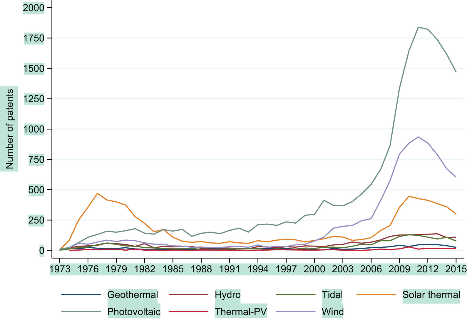
Number of patents filed by REG category.
4.3 TTs’ Identification
To use TVD, we need the number of periods within the whole sample and the distance between them. Thus, we define the periods using two criteria, natural periods and PSNO, which we describe in the following paragraphs.
We first divide our data by natural years, each constituting a “natural period”; then, we select the distance of comparison between natural periods. The distributions may look very similar when periods are too short and the distances too close. Therefore, shorter periods may need further distance calculations. We test a variety of combinations of years and periods of distance. Interestingly, we obtain high consistency in defining two TT moments in the REG case: one in the 1980s and another between the end of the 1990s and the beginning of the 2000s.
In Figure 2, we show different year-windows and the distance between them. If we take 1-year periods and calculate the distances between five periods, we identify two peaks (Figure 2(a)). The first peak compares the distribution in 1981 with one in 1986. The second one signals a peak in the distance between the distribution in 1997 and the one in 2002. The graph with 2-year periods with comparisons of two period distance (Figure 2(b)) exhibits more clearly the two peaks: the first one compares the distribution of 1981–1982 with 1984–1985; the second one compares the 1998–1999 distribution with that of 2002–2003. In Figure 2(c), we again observe the two peaks in the 3-year periods with consecutive (distance 1) comparisons: 1983–1985 with 1986–1989, and 2000–2002 with 2003–2005. The 5-year periods with consecutive comparisons, Figure 2(d), give a similar picture, with a first peak in 1978–1982 compared with 1983–1987, and the second comparing 1998–2002 to 2003–2007.

TVD for natural periods: (a) 1-year periods with five-period distance, (b) 2-year periods with two-period distance, (c) 3-year periods consecutive, and (d) 5-year periods consecutive.
For illustration purposes, in Figure 3, we show the histograms for 5-year natural periods comparing 1978–1982 and 1983–1987 (Figure 3(a)) and 1998–2002 and 2003–2007 (Figure 3(b)), which are associated with the two red points of Figure 5(d). The most notorious change from 1978–1982 to 1983–1987 is a relative reduction of subgroup 4 (solar-thermal) and an increase in subgroup 5 (PV). During the second peak, from 1998–2002 to 2003–2007, we observe a relative reduction of subgroups 4 and 5, which transition to an increase of subgroup 7 (wind).
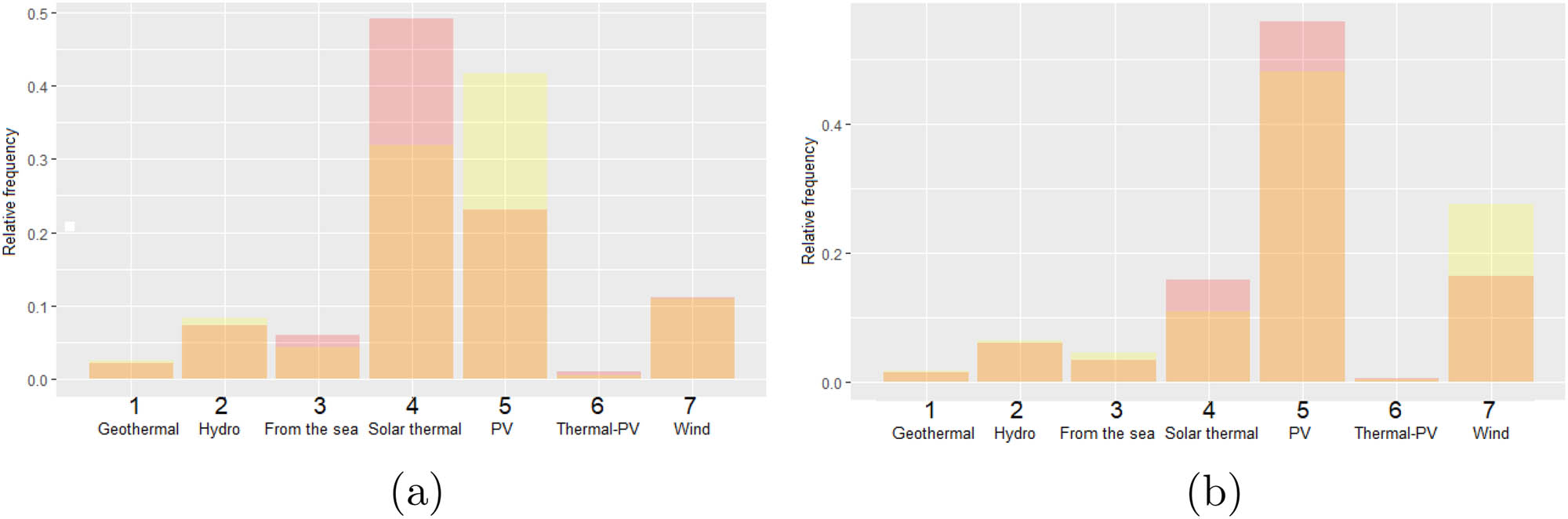
Distributions during TT for 5-year natural periods: (a) distributions during 1978–1982 (red) and 1983–1987 (yellow) and common (orange) and (b) distributions during 1998–2002 (red) and 2003–2007 (yellow) and common (orange).
We repeat the exercise for PSNO Figure 4. In this way, we correct for a variability bias due to the greater number of patents being registered in recent years. Similar to the case of natural periods, a greater number of periods would result in shorter periods, which would demand a comparison conceding a greater distance.

TVD for PSNO: (a) 40 PSNO consecutive, (b) 40 PSNO with three-period distance, (c) 30 PSNO consecutive, and (d) 25 PSNO consecutive.
If we consider 40 PSNO and a consecutive comparison (Figure 4(a)), we find two notable peaks: one between June 1982 and March 1988,[14] and the second between March 2000 and April 2003.[15] For the same 40 PSNO and a comparison of distance 3 (Figure 4(b)), we obtain the same two peaks: one between June 1979 and March 1988,[16] and the second, between January 1995 and April 2003.[17] For 30 PSNO with a consecutive comparison (Figure 4(c)), we obtain two main peaks between October 1980 and December 1986,[18] and between June 1999 and October 2003.[19] For 25 PSNO (Figure 4(d)), the identification is less precise: one between October 1980 and December 1991[20] and the second between October 1997 and August 2004.[21]
For robustness, we performed a multinomial chi-square test of independence between each pair of distributions to test whether these two come from the same distribution.[22] If we assume that the realization of patents in a particular year is a “sample,” in the absence of technological change, the relative distribution of patents among the categories must be the same between the two periods.
Thus, by performing the independence test between two samples, we are testing whether these two belong to the same population, and when we reject this null hypothesis, there has been technological change. However, as we explained earlier, we are interested in finding those moments with a drastic technological change; thus, if the test statistic is much larger than the critical value, then it would signal a TT.
Since the chi-square test of independence is affected by the size of each sample, we only performed it on the distributions grouped in natural years. Also, we did not have extreme values for the frequency distributions of most of the natural (and synthetic) periods analyzed; thus, this multinomial test performed satisfactorily, and we found no need to introduce additional tests (see Cai & Krishnamoorthy, 2006).
In Figure 5, we offer a comparable graph for Figure 2 of the chi-square statistics for every paired of distributions. Also, we show two levels of significance

Multinominal chi test: (a) 1-year periods with five-period distance, (b) 2-year periods with two-period distance, (c) 3-year periods consecutive, and (d) 5-year periods consecutive.
The TTs identified correspond very consistently to local maxima of the statistic. In the first graph, the first TT, at the pair 1981–1986, coincides with a local maximum of the statistic with a value of 77.2952 that corresponds to a
In this section, we show that the TVD approach has consistently identified two TTs, despite considering a wide range of period sizes and comparison distances. Note that since we have not considered any external information, the measure is ideal for an initial exploratory analysis and only uses the relative frequency of each category within REG field.
4.4 Interpretation
Our methodology systematically indicates two moments of notable change in the distribution of patents for REG. Although TTs could have occurred naturally, we aim to acknowledge some policies linked to the two moments identified through the TVD calculation, which qualitatively reinforce the correct identification of the TTs. The first peak in the early 1980s could result from the research that would have started in the late 1970s. Between the late 1990s and the beginning of the 2000s, the second peak could relate to the Kyoto Treaty. However, we do not pretend to establish any causality between the policies mentioned and the TTs.
The oil embargo of 1973 triggered interest in alternative energies, which motivated a wide range of energy conversion techniques from renewable sources. Among these, PV panels started to be considered a viable option for commercial use (Sørensen, 1991). The oil crisis in the 1970s triggered public funding for R&D programs aimed to advance PV generation, mainly from Japan and the USA, and it is calculated that around 60% of the cost reduction in this technology was due to public and private R&D (International Energy Agency, 2020). President Nixon’s Project Independence in 1973, President Ford’s Energy Policy and Conservation Act in 1975, and the Public Utility Regulatory Policies Act in 1978 also promoted renewables and have been related to technological changes that led to cost reductions in wind and solar PV (Clayton, 2004; Smith, 2004; Solomon & Krishna, 2011).
In 1997, the Kyoto Protocol was adopted by almost 200 countries, committing the signers to reduce their carbon emissions by 2012. Evidence suggests that the protocol triggered a rapid increase in patenting activity in CCMTs. A positive effect has been found on applications for renewable technology patents in countries with emission targets (Miyamoto & Takeuchi, 2019). This increase has significantly affected solar and wind technology patents in European countries (Johnstone et al., 2010). Even though the USA signed the protocol on November 12, 1998, the treaty was never ratified by the US Senate, as needed.
However, the protocol could have awakened economic incentives in other countries that had signed and ratified the protocol, which led to increased interest in patenting in the US. Also, US polls on political concerns and political initiatives, such as President Clinton’s tax on BTUs proposal, or the Climate Change Action Plan, indicated potential changes in energy regulation in favor of renewable sources. Chalvatzis et al. (2020) argue that the Kyoto Protocol redirected innovation efforts towards REG, promoting the interest of the corresponding R&D to meet the growing demand in that sector. The prevailing dominant positions in the patenting of PV and wind could reflect the extensive use of these technologies in the marketplace (UNEP et al., 2010).
5 Final Comments
As we have seen, TVD is commonly used in measure theory, computation, and the natural sciences. However, this article provides evidence that TVD is a useful exploratory tool for measuring and detecting TTs based solely on patent data. We use the information of a particular technology’s entire probability density distribution instead of focusing on specific subgroup trends. Since the methodology does not depend on any additional information apart from patent documents, it is ideal for analyzing a given technology’s evolution.
This article provides two main insights. On the one hand, we first apply a distribution distance to the categories of a technological field to measure technological change. On the other hand, since we focus on temporal changes, we propose a methodology to identify tipping points in different systems, not only for technology. Furthermore, we contrast the results of the TVD to a multinomial chi-square test of independence, and the results are mostly in line, except for a third maximum that the chi-square identified, which was driven by the growth of the sample size and not due to a big change in composition within the REG technology, which is precisely what the TVD approach measures.
Our proposed methodology might be applied to identify a regime change, for instance, an ecosystem regime change. However, the optimal application requires keeping the same categories within the whole evaluation period, or reorganizing the data for new categorizations, as in the REG case. We use an exogenous classification for the technology; however, the same methodology applies once a researcher has developed non-ordered categorical variables containing each patent.
One limitation of using TVD on distributions over technological categories is that we are not considering the technological distance between those categories. We are assuming, for example, the same technological distance between solar thermal and solar PV as between solar thermal and wind energy generation. Nevertheless, the relative distribution of multiple assigned patents seems to indicate that this is not the case. Including such a dimension, even if it is not done using distances over distributions, may offer a more sensitive indicator to signal TTs.
We acknowledge that a TT is a complex phenomenon and that the distribution of categories within a particular technological field may not completely describe it. For instance, Antal et al. (2017) suggest that energy transitions involve highly complex processes involving different actors (government, private firms, and research institutions) and regime shifts that depend on energy resources and infrastructure to utilize and benefit from them. However, since this methodology has low information requirements, it is helpful for exploratory and visual analysis.
Finally, since we focus only on the relative frequency of patents, and each patent may have a different value, an extension of this article could be to calculate a measure that assigns different weights to each patent so that the pdf approximates a value distribution across the corresponding subgroups.
Acknowledgments
The authors are grateful with Tomas Bocanegra, librarian of El Colegio de Mexico, for his help finding some of the references.
-
Funding information: The authors did not receive support from any organization for the submitted work.
-
Conflict of interest: All authors declare that they have no conflicts of interest.
-
Article note: As part of the open assessment, reviews and the original submission are available as supplementary files on our website.
Appendix Y02E 10 Classification Scheme
| Y02E 10/10 |
|
| Y02E 10/12 |
|
| Y02E 10/125 |
|
| Y02E 10/14 |
|
| Y02E 10/16 |
|
| Y02E 10/18 |
|
| Y02E 10/20 |
|
| Y02E 10/22 |
|
| Y02E 10/223 |
|
| Y02E 10/226 |
|
| Y02E 10/28 |
|
| Y02E 10/30 |
|
| Y02E 10/32 |
|
| Y02E 10/34 |
|
| Y02E 10/36 |
|
| Y02E 10/38 |
|
| Y02E 10/40 |
|
| Y02E 10/41 |
|
| Y02E 10/42 |
|
| Y02E 10/43 |
|
| Y02E 10/44 |
|
| Y02E 10/45 |
|
| Y02E 10/46 |
|
| Y02E 10/465 |
|
| Y02E 10/47 |
|
| Y02E 10/50 |
|
| Y02E 10/52 |
|
| Y02E 10/54 |
|
| Y02E 10/541 |
|
| Y02E 10/542 |
|
| Y02E 10/543 |
|
| Y02E 10/544 |
|
| Y02E 10/545 |
|
| Y02E 10/546 |
|
| Y02E 10/547 |
|
| Y02E 10/548 |
|
| Y02E 10/549 |
|
| Y02E 10/56 |
|
| Y02E 10/563 |
|
| Y02E 10/566 |
|
| Y02E 10/58 |
|
| Y02E 10/60 |
|
| Y02E 10/70 |
|
| Y02E 10/72 |
|
| Y02E 10/721 |
|
| Y02E 10/722 |
|
| Y02E 10/723 |
|
| Y02E 10/725 |
|
| Y02E 10/726 |
|
| Y02E 10/727 |
|
| Y02E 10/728 |
|
| Y02E 10/74 |
|
| Y02E 10/76 |
|
| Y02E 10/763 |
|
| Y02E 10/766 |
|
References
Absalom, R., Förster, W., Galan, E. M., Scheu, M., Veefkind, V., & Verbandt, Y. (2006). Mapping nanotechnology patents: The EPO approach. World Patent Information, 28(3), 204–211. 10.1016/j.wpi.2006.03.005Suche in Google Scholar
Alkemade, F., Heimeriks, G., Hoekstra, R., & Leydesdorff, L. (2015). Patents as instruments for exploring innovation dynamics: Geographic and technological perspectives on “photovoltaic cells”. Scientometrics, 102(1), 629–651. 10.1007/s11192-014-1447-8Suche in Google Scholar
Angelucci, S., Hurtado-Albir, J., Karachalios, K., Thumm, N., & Veefkind, V. (2012). A new EPO classification scheme for climate change mitigation technologies. World Patent Information, 34(2), 106–111. 10.1016/j.wpi.2011.12.004Suche in Google Scholar
Antal, M., Cherp, A., Jewell, J., Suzuki, M., & Vinichenko, V. (2017). Comparing electricity transitions: A historical analysis of nuclear, wind and solar power in Germany and Japan. Energy Policy, 101(May 2016), 612–628. 10.1016/j.enpol.2016.10.044Suche in Google Scholar
Bae, J., & Kim, G. (2017). A novel approach to forecast promising technology through patent analysis. Technological Forecasting and Social Change, 117, 228–237. 10.1016/j.techfore.2016.11.023Suche in Google Scholar
Ball, F., & Donnelly, P. (1995). Strong approximations for epidemic models. Stochastic Processes and Their Applications, 55(1), 1–21. 10.1016/0304-4149(94)00034-QSuche in Google Scholar
Barger, Z., Frye, C. G., Liu, D., Dan, Y., & Bouchard, K. E. (2019). Robust, automated sleep scoring by a compact neural network with distributional shift correction. PLoS ONE, 14(12), 1–18. 10.1371/journal.pone.0224642Suche in Google Scholar
Cai, Y., & Krishnamoorthy, K. (2006). Exact size and power properties of five tests for multinomial proportions. Communications in Statistics Simulation and Computation RRR, 35(1), 149–160. 10.1080/03610910500415993Suche in Google Scholar
Carte, K. M., Lu, M., Luo, Q., Jiang, H., & An, L. (2020). Microbial community dissimilarity for source tracking with application in forensic studies. PLoS ONE, 15(7 July), 1–17. 10.1371/journal.pone.0236082Suche in Google Scholar
Cha, S. H., & Srihari, S. N. (2002). On measuring the distance between histograms. Pattern Recognition, 35(6), 1355–1370. 10.1016/S0031-3203(01)00118-2Suche in Google Scholar
Chalvatzis, K., Pitelis, A., & Vasilakos, N. (2020, May). Fostering innovation in renewable energy technologies: Choice of policy instruments and effectiveness. Renewable Energy, 151, 1163–1172. 10.1016/j.renene.2019.11.100Suche in Google Scholar
Clayton, M. (2004). Solar power hits suburbia. The Christian Science Monitor. Suche in Google Scholar
Duda, R. O., Hart, P. E., & Stork, D. G. (2007). Pattern Classification (2nd ed.). Wiley. Suche in Google Scholar
EPO & USPTO. (2015). Guide to the CPC Cooperative Patent Classification. Suche in Google Scholar
Euán, C., Ombao, H., & Ortega, J. (2018). The hierarchical spectral merger algorithm: A new time series clustering procedure. Journal of Classification, 35(1), 71–99. 10.1007/s00357-018-9250-5Suche in Google Scholar
Frenken, K., Kupers, R., & Zeppini, P. (2014). Thresholds models of technological transitions. Environmental Innovation and Societal Transitions, 11, 54–70. 10.1016/j.eist.2013.10.002Suche in Google Scholar
Garcia, S. P., & Pinho, A. J. (2011). Minimal absent words in four human genome assemblies. PLoS ONE, 6(12), 1–11. 10.1371/journal.pone.0029344Suche in Google Scholar
Guderian, C. C. (2019). Identifying emerging technologies with smart patent indicators: The example of smart houses. International Journal of Innovation and Technology Management, 16(2), 1–24. 10.1142/S0219877019500408Suche in Google Scholar
International Energy Agency. (2020). Special Report on Clean Energy Innovation: Accelerating technology progress for a sustainable future. Technical report. Suche in Google Scholar
Johnstone, N., Haščič, I., & Popp, D. (2010). Renewable energy policies and technological innovation: Evidence based on patent counts. Environmental and Resource Economics, 45(1), 133–155. 10.1007/s10640-009-9309-1Suche in Google Scholar
Kurtz, C., Gançarski, P., Passat, N., & Puissant, A. (2013). A hierarchical semantic-based distance for nominal histogram comparison. Data and Knowledge Engineering, 87, 206–225. 10.1016/j.datak.2013.06.002Suche in Google Scholar
Lacasa, I. D., Grupp, H., & Schmoch, U. (2003). Tracing technological change over long periods in Germany in chemicals using patent statistics. Scientometrics, 57(2), 175–195. 10.1023/A:1024133517484Suche in Google Scholar
Lin, D., Liu, W., Guo, Y., & Meyer, M. (2021). Using technological entropy to identify technology life cycle. Journal of Informetrics, 15(2), 101137. 10.1016/j.joi.2021.101137Suche in Google Scholar
Lobo, J., & Strumsky, D. (2019). Sources of inventive novelty: Two patent classification schemas, same story. Scientometrics, 120(1), 19–37. 10.1007/s11192-019-03102-2Suche in Google Scholar
Lobo, J., Strumsky, D., & van der Leeuw, S. (2012). Using patent technology codes to study technological change. Economics of Innovation and New Technology, 21(3), 267–286. 10.1080/10438599.2011.578709Suche in Google Scholar
Martino, J. (1971). Examples of technological trend forecasting for research and development planning. Technological Forecasting and Social Change, 2(3–4), 247–260. 10.1016/0040-1625(71)90003-5Suche in Google Scholar
Massart, P. (2007). Concentration inequalities and model selection (Vol. 6). Springer. Suche in Google Scholar
Meguro, K., & Osabe, Y. (2019). Lost in patent classification. World Patent Information, 57, 70–76. 10.1016/j.wpi.2019.03.008Suche in Google Scholar
Miyamoto, M., & Takeuchi, K. (2019). Climate agreement and technology diffusion: Impact of the kyoto protocol on international patent applications for renewable energy technologies. Energy Policy, 129, 1331–1338. 10.1016/j.enpol.2019.02.053Suche in Google Scholar
Perez-Molina, E., & Loizides, F. (2021). Novel data structure and visualization tool for studying technology evolution based on patent information: The DTFootprint and the TechSpectrogram. World Patent Information, 64(April 2020), 102009. 10.1016/j.wpi.2020.102009Suche in Google Scholar
Popp, D., Juhl, T., & Johnson, D. K. (2004). Time in purgatory: Examining the grant lag for us patent applications. The BE Journal of Economic Analysis and Policy, 4(1), 1–45. 10.2202/1538-0653.1329Suche in Google Scholar
Ruijie, Z., Ying, X., Shuaichen, J., & Yonghe, L. (2021). Patent text modeling strategy and its classification based on structural features. World Patent Information, 67, 102084. 10.1016/j.wpi.2021.102084Suche in Google Scholar
Smith, R. (2004). Not just tilting anymore: Higher fuel costs, tax credits, better technology whip up hopes for wind power again. The Wall Street Journal, 1. https://www.wsj.com/articles/SB109770528042944636.Suche in Google Scholar
Solomon, B. D., & Krishna, K. (2011). The coming sustainable energy transition: History, strategies, and outlook. Energy Policy, 39(11), 7422–7431. 10.1016/j.enpol.2011.09.009Suche in Google Scholar
Sørensen, B. (1991). A history of renewable energy technology. Energy policy, 19(1), 8–12. 10.1016/0301-4215(91)90072-VSuche in Google Scholar
Strelkov, V. V. (2008). A new similarity measure for histogram comparison and its application in time series analysis. Pattern Recognition Letters, 29(13), 1768–1774. 10.1016/j.patrec.2008.05.002Suche in Google Scholar
Sung-Hyuk, C. (2007). Comprehensive survey on distance/similarity measures between probability density functions. International Journal of Mathematical Models and Methods in Applied Sciences, 1(4), 300–307. Suche in Google Scholar
UNEP, EPO, & ICTSD. (2010). Patents and clean energy: Bridging the gap between evidence and policy. Technical report. Suche in Google Scholar
© 2023 the author(s), published by De Gruyter
This work is licensed under the Creative Commons Attribution 4.0 International License.
Artikel in diesem Heft
- Regular Articles
- Export Cutoff Productivity, Uncertainty and Duration of Waiting for Exporting
- Survival of the Fittest: The Long-run Productivity Analysis of the Listed Information Technology Companies in the US Stock Market
- A Replication of “The Effect of the Conservation Reserve Program on Rural Economies: Deriving a Statistical Verdict from a Null Finding” (American Journal of Agricultural Economics, 2019)
- An Alternative Approach to Frequency of Patent Technology Codes: The Case of Renewable Energy Generation
- Environmental Taxation and International Trade in a Tax-Distorted Economy
- Foreign Investors and the Peer Effects to Payout Policies
- Segregation, Education Cost, and Group Inequality
- Does the Different Ways of Internet Utilization Promote Entrepreneurship: Evidence from Rural China
- Reinvestigating the U.S. Consumption Function: A Nonlinear Autoregressive Distributed Lags Approach
- Regional Environment Risk Assessment Over Space and Time: A Case of China
- Unraveling Producer Price Inflation Pass-Through: Quantification, Structural Breaks, and Causal Direction
- The Relationship Between Knowledge Risk Management and Sustainable Organizational Performance: The Mediating and Moderating Role of Leadership Behavior
- Special Issue: Data Governance in the Digital Era
- From Competition Law to Platform Regulation – Regulatory Choices for the Digital Markets Act
- IP Law and Policy for the Data Economy in the EU
- Is Data the New Gold? Considering Intellectual Property Protection and Regulation of Data
- Special Issue: Shapes of Performance Evaluation in Economics and Management Decision - Part I
- Path Constitution: Building Organizational Resilience for Sustainable Performance
- An Evaluation of E7 Countries’ Sustainable Energy Investments: A Decision-Making Approach with Spherical Fuzzy Sets
- Special Issue: Economic Implications of Management and Entrepreneurship - Part I
- Organizational Integration, Knowledge Management, and Sustainable Entrepreneurship for SMEs in Developing Economies
- Does Bitcoin Affect Term Deposits? Evidence from MINT Countries
- Effects of Social Responsibility Practices on the Brand Image, Brand Awareness, and Brand Loyalty of Sponsor Businesses: A Study on Sports Clubs
- The Effect of Market and Technological Turbulence on Innovation Performance in Nascent Enterprises: The Moderating Role of Entrepreneur’s Courage