Faster approximation to multivariate functions by combined Bernstein-Taylor operators
-
Oktay Duman


Abstract
In this article, we incorporate multivariate Taylor polynomials into the definition of the Bernstein operators to get a faster approximation to multivariate functions by these combined operators. We also give various numerical simulations including graphical illustrations and error estimations. Our results improve not only the linear approximation by classical Bernstein polynomials but also the nonlinear approximation obtained by max-product operations.
1 Introduction
The approximation of multivariate functions using Bernstein polynomials is a well-established topic. In this article, we focus on enhancing the rate of approximation by modifying Bernstein polynomials with the help of Taylor polynomials. The initial idea in this direction was introduced by Kirov [1] for the approximation of univariate functions. In this article, we first extend Kirov’s approach to the multivariate case, developing a framework to approximate multivariate functions more effectively. Second, we apply the same method to the nonlinear Bernstein operators modified using max-product operations. These modifications also lead to improved approximation results compared to the classical case. Our findings are supported by graphical representations and numerical values, which illustrate the superiority of the proposed modifications over the classical Bernstein operators.
In the classical approximation theory, one of the most effective known methods for (uniformly) approximating a multivariate function
for
It is well known that the rate of convergence for approximation to continuous functions by Bernstein polynomials is of order
As usual, for a given
With this terminology, the combined Bernstein-Taylor operators are defined by
for
Another important aspect of this work is that we will also obtain similar results for nonlinear Bernstein operators. Recall that if we replace the sum operation
for
holds for
for
2 Approximation by combined Bernstein-Taylor operators in (1.2) and (1.4)
Let
for
Lemma 2.1
For
where the positive constant D depends only on m and
Proof
We observe from (1.1) that
where
holds for a constant
In our recent paper [14], using the concept of modulus of continuity
we have also proved the next lemma.
Lemma 2.2
[14] For
for some
Now using the supremum norm
Theorem 2.1
Let
where the positive constant C depends only upon m and r. Then, for every
Proof
We first observe that the result is clear for
holds. Letting
for some
Now Lemma 2.1 implies that
holds for some constant
Remark 2.1
From Theorem 2.1 if
This clearly shows that approximation to functions by our combined operators
Remark 2.2
By a simple translation in Theorem 2.1, we can also take any hyperrectangle
the corresponding combined Bersntein-Taylor operators become
where
for
Now, we focus on the approximation by the combined operators
Lemma 2.3
For
where the positive constant D depends only upon m and
Proof
As in the proof of Lemma 2.1, we may write that
where
is satisfied for each
Now combining the above results and also taking
Then, we obtain the following result.
Theorem 2.2
Let
for some
Proof
The case of
holds for some
for some positive constant
3 Numerical simulations
In this section, we give some numerical simulations of Theorems 2.1 and 2.2. Now let
for
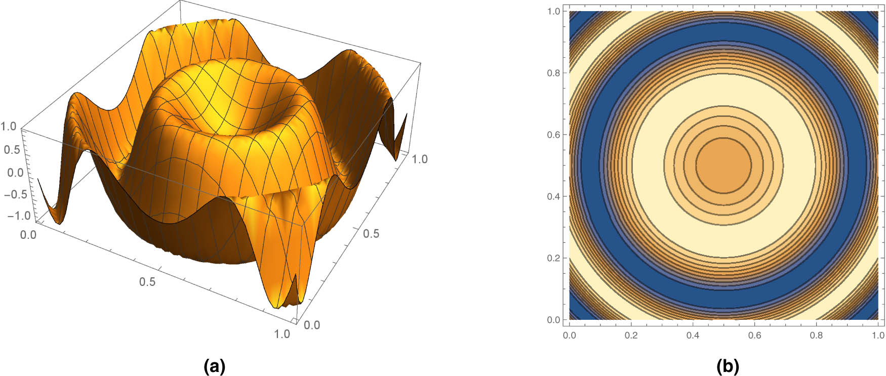
Graph of the target function
![Figure 2
Approximation to
f
f
by
B
n
[
r
]
(
f
)
{{\mathbb{B}}}_{n}^{\left[r]}(f)
: (a)
r
=
0
r=0
and
n
=
5
n=5
, 10, 15, respectively, (b)
r
=
1
r=1
and
n
=
5
n=5
, 10, 15, respectively, and (c)
r
=
2
r=2
and
n
=
5
n=5
, 10, 15, respectively.](/document/doi/10.1515/dema-2025-0129/asset/graphic/j_dema-2025-0129_fig_002.jpg)
Approximation to
![Figure 3
Level curves in the approximation to
f
f
by
B
n
[
r
]
(
f
)
{{\mathbb{B}}}_{n}^{\left[r]}(f)
: (a)
r
=
0
r=0
and
n
=
5
n=5
, 10, 15 respectively, (b)
r
=
1
r=1
and
n
=
5
n=5
, 10, 15, respectively, and (c)
r
=
2
r=2
and
n
=
5
n=5
, 10, 15, respectively.](/document/doi/10.1515/dema-2025-0129/asset/graphic/j_dema-2025-0129_fig_003.jpg)
Level curves in the approximation to
Now it is also possible to calculate numerically the errors in this approximation. By using the absolute error
for the values of
Pointwise errors in the approximation
| (a) The mean errors | ||
|---|---|---|
|
|
|
|
| 20 | 0.4210173 | 0.3787726 |
| 40 | 0.2767969 | 0.2054019 |
| 80 | 0.1609748 | 0.0779949 |
| (b) The mean sequare errors | ||
|---|---|---|
|
|
|
|
| 20 | 0.4749271 | 0.4220906 |
| 40 | 0.3152598 | 0.2344957 |
| 80 | 0.1855133 | 0.0918319 |
Finally, to observe the approximation in Theorem 2.2, we choose the following target function
for
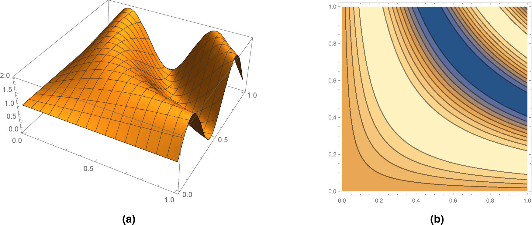
Graph of the target function
![Figure 5
Approximation to
g
g
by
B
n
[
r
,
M
]
(
g
)
{{\mathbb{B}}}_{n}^{\left[r,M]}\left(g)
: (a)
r
=
0
r=0
and
n
=
5
n=5
, 10, 15, respectively, (b)
r
=
1
r=1
and
n
=
5
n=5
, 10, 15, respectively, and (c)
r
=
2
r=2
and
n
=
5
n=5
, 10, 15, respectively.](/document/doi/10.1515/dema-2025-0129/asset/graphic/j_dema-2025-0129_fig_005.jpg)
Approximation to
![Figure 6
Level curves in the approximation to
g
g
by
B
n
[
r
,
M
]
(
g
)
{{\mathbb{B}}}_{n}^{\left[r,M]}\left(g)
: (a)
r
=
0
r=0
and
n
=
5
n=5
, 10, 15, respectively, (b)
r
=
1
r=1
and
n
=
5
n=5
, 10, 15, respectively, and (c)
r
=
2
r=2
and
n
=
5
n=5
, 10, 15, respectively.](/document/doi/10.1515/dema-2025-0129/asset/graphic/j_dema-2025-0129_fig_006.jpg)
Level curves in the approximation to
4 Concluding remarks
By using multivariate Taylor polynomials, we have modified the classical Bernstein polynomial and its nonlinear version based on max-product operations. These modifications enable us to obtain more efficient approximation results than (linear and nonlinear) Bernstein operators.
It is important to note that while this modification significantly improves the approximation speed, it also introduces additional computational complexity depending on the choice of the Taylor polynomial with degree
We should also note that, so far, such modifications have been focused more on Shepard operators by using not only Taylor polynomials but also Bernoulli, Lidstone, and Hermite polynomials [14–18]. Therefore, it will be interesting to develop Bernstein operators with these polynomials in future research. In addition, further investigations into optimizing the balance between computational complexity and convergence rate could enhance the practical applicability of the proposed method.
Acknowledgements
The author would like to express his gratitude to the reviewers for their insightful comments and suggestions, which have improved the clarity and impact of this work.
-
Funding information: Author states no funding involved.
-
Author contributions: The author confirms the sole responsibility for the conception of the study, presented results and manuscript preparation.
-
Conflict of interest: Prof. Oktay Duman is a member of the Editorial Board of the journal Demonstratio Mathematica, but was not involved in the review process of this article.
-
Ethical approval: The conducted research is not related to either human or animals use.
-
Data availability statement: Not applicable.
References
[1] G. H. Kirov, A generalization of the Bernstein polynomials, Math. Balkanica (N.S.) 6 (1992), no. 2, 147–153, http://www.math.bas.bg/infres/MathBalk/MB-06/MB-06-147-153.pdf. Suche in Google Scholar
[2] U. Abel, V. Gupta, and R. N. Mohapatra, Local approximation by a variant of Bernstein-Durrmeyer operators, Nonlinear Anal. 68 (2008), no. 11, 3372–3381, DOI: https://doi.org/10.1016/j.na.2007.03.026. 10.1016/j.na.2007.03.026Suche in Google Scholar
[3] A. J. Adell and D. Cárdenas-Morales, Stochastic Bernstein polynomials: uniform convergence in probability with rates, Adv. Comput. Math. 46 (2020), no. 2, Paper No. 16, 10pp, DOI: https://doi.org/10.1007/s10444-020-09770-6. 10.1007/s10444-020-09770-6Suche in Google Scholar
[4] F. Altomare and M. Campiti, Korovkin-Type Approximation Theory and its Applications, De Gruyter Studies in Mathematics, vol. 17, Walter de Gruyter and Co., Berlin, 1994. 10.1515/9783110884586Suche in Google Scholar
[5] G. A. Anastassiou and S. G. Gal, Approximation Theory, Birkhäuser Boston, Inc., Boston, MA, 2000. 10.1007/978-1-4612-1360-4Suche in Google Scholar
[6] C. Bardaro, P. L. Butzer, R. L. Stens, and G. Vinti, Convergence in variation and rates of approximation for Bernstein-type polynomials and singular convolution integrals, Analysis 23 (2003), no. 4, 299–340, DOI: https://doi.org/10.1524/anly.2003.23.4.299. 10.1524/anly.2003.23.4.299Suche in Google Scholar
[7] B. Bede, L. Coroianu, and S. G. Gal, Approximation and shape preserving properties of the Bernstein operator of max-product kind, Int. J. Math. Math. Sci. 2009 (2009), no. 1, 590589, DOI: https://doi.org/10.1155/2009/590589. 10.1155/2009/590589Suche in Google Scholar
[8] B. Bede, L. Coroianu, and S. G. Gal, Approximation by Max-Product Type Operators, Springer, Cham, 2016. 10.1007/978-3-319-34189-7Suche in Google Scholar
[9] M. Campiti and I. Raşa, Extrapolation properties of multivariate Bernstein polynomials, Mediterr. J. Math. 16 (2019), no. 5, 109, DOI: https://doi.org/10.1007/s00009-019-1392-0. 10.1007/s00009-019-1392-0Suche in Google Scholar
[10] D. Cárdenas-Morales, M. Jiménez-Pozo, and F. J. Munnnnoz-Delgado, Some remarks on Hölder approximation by Bernstein polynomials, Appl. Math. Lett. 19 (2006), no. 10, 1118–1121, DOI: https://doi.org/10.1016/j.aml.2005.11.024. 10.1016/j.aml.2005.11.024Suche in Google Scholar
[11] N. I. Mahmudov, Approximation by Bernstein-Durrmeyer-type operators in compact disks, Appl. Math. Lett. 24 (2011), no. 7, 1231–1238, DOI: https://doi.org/10.1016/j.aml.2011.02.014. 10.1016/j.aml.2011.02.014Suche in Google Scholar
[12] S. Ostrovska, q-Bernstein polynomials and their iterates, J. Approx. Theory 123 (2003), no. 2, 232–255, DOI: https://doi.org/10.1016/S0021-9045(03)00104-7. 10.1016/S0021-9045(03)00104-7Suche in Google Scholar
[13] G. G. Lorentz, Bernstein Polynomials, 2nd ed. AMS Chelsea Pub. Co., New York, 1986. Suche in Google Scholar
[14] O. Duman, Max-product Shepard operators based on multivariable Taylor polynomials, J. Comput. Appl. Math. 437 (2024), 115456, DOI: https://doi.org/10.1016/j.cam.2023.115456. 10.1016/j.cam.2023.115456Suche in Google Scholar
[15] R. Farwig, Rate of convergence of Shepardas global interpolation formula, Math. Comp. 46 (1986), no. 174, 577–590, DOI: https://doi.org/10.2307/2007995. 10.1090/S0025-5718-1986-0829627-0Suche in Google Scholar
[16] R. Caira and F. Dell’Accio, Shepard-Bernoulli operators, Math. Comp. 76 (2007), no. 257, 299–321, DOI: https://doi.org/10.1090/S0025-5718-06-01894-1. 10.1090/S0025-5718-06-01894-1Suche in Google Scholar
[17] R. Caira, F. Dell’Accio, and F. Di Tommaso, On the bivariate Shepard-Lidstone operators, J. Comput. Appl. Math. 236 (2012), no. 7, 1691–1707, DOI: https://doi.org/10.1016/j.cam.2011.10.001. 10.1016/j.cam.2011.10.001Suche in Google Scholar
[18] F. A. Costabile, F. Dell’Accio, and F. Di Tommaso, Enhancing the approximation order of local Shepard operators by Hermite polynomials, Comput. Math. Appl. 64 (2012), no. 11, 3641–3655, DOI: https://doi.org/10.1016/j.camwa.2012.10.004. 10.1016/j.camwa.2012.10.004Suche in Google Scholar
© 2025 the author(s), published by De Gruyter
This work is licensed under the Creative Commons Attribution 4.0 International License.
Artikel in diesem Heft
- Research Articles
- On approximation by Stancu variant of Bernstein-Durrmeyer-type operators in movable compact disks
- Circular n,m-rung orthopair fuzzy sets and their applications in multicriteria decision-making
- Grand Triebel-Lizorkin-Morrey spaces
- Coefficient estimates and Fekete-Szegö problem for some classes of univalent functions generalized to a complex order
- Proofs of two conjectures involving sums of normalized Narayana numbers
- On the Laguerre polynomial approximation errors and lower type of entire functions of irregular growth
- New convolutions for the Hartley integral transform imbedded in the Banach algebras and convolution-type integral equations
- Some inequalities for rational function with prescribed poles and restricted zeros
- Lucas difference sequence spaces defined by Orlicz function in 2-normed spaces
- Evaluating the efficacy of fuzzy Bayesian networks for financial risk assessment
- Fixed point results for contractions of polynomial type
- Estimation for spatial semi-functional partial linear regression model with missing response at random
- Investigating the controllability of differential systems with nonlinear fractional delays, characterized by the order 0 < η ≤ 1 < ζ ≤ 2
- New forms of bilateral inequalities for K-g-frames
- Rate of pole detection using Padé approximants to polynomial expansions
- Existence results for nonhomogeneous Choquard equation involving p-biharmonic operator and critical growth
- Note on the shape-preservation of a new class of Kantorovich-type operators via divided differences
- Geršhgorin-type theorems for Z1-eigenvalues of tensors with applications
- New topologies derived from the old one via operators
- Blow up solutions for two-dimensional semilinear elliptic problem of Liouville type with nonlinear gradient terms
- Infinitely many normalized solutions for Schrödinger equations with local sublinear nonlinearity
- Nonparametric expectile shortfall regression for functional data
- Advancing analytical solutions: Novel wave insights and methodologies for beta fractional Kuralay-II equations
- A generalized p-Laplacian problem with parameters
- A study of solutions for several classes of systems of complex nonlinear partial differential difference equations in ℂ2
- Towards finding equalities involving mixed products of the Moore-Penrose and group inverses by matrix rank methodology
-
- Coefficient functionals for Sakaguchi-type-Starlike functions subordinated to the three-leaf function
- Solutions of several general quadratic partial differential-difference equations in ℂ2
- Inequalities for the generalized trigonometric functions with respect to weighted power mean
- Optimization of Lagrange problem with higher-order differential inclusion and special boundary-value conditions
- Hankel determinants for q-starlike functions connected with q-sine function
- System of partial differential hemivariational inequalities involving nonlocal boundary conditions
- A new family of multivalent functions defined by certain forms of the quantum integral operator
- A matrix approach to compare BLUEs under a linear regression model and its two competing restricted models with applications
- Weighted composition operators on bicomplex Lorentz spaces with their characterization and properties
- Behavior of spatial curves under different transformations in Euclidean 4-space
- Commutators for the maximal and sharp functions with weighted Lipschitz functions on weighted Morrey spaces
- A new kind of Durrmeyer-Stancu-type operators
- A study of generalized Mittag-Leffler-type function of arbitrary order
- On the approximation of Kantorovich-type Szàsz-Charlier operators
- Split quaternion Fourier transforms for two-dimensional real invariant field
- Quantum injectivity of G-frames in Hilbert spaces
- Some results on disjointly weakly compact sets
- On Motzkin sequence spaces via q-analog and compact operators
- Existence and multiplicity of nontrivial solutions for Schrödinger-Bopp-Podolsky systems with critical nonlinearity in ℝ3
- Stability analysis of linear time-invariant difference-differential system with constant and distributed delays
- The discriminant of quasi m-boundary singularities
- Review Article
- Characterization generalized derivations of tensor products of nonassociative algebras
- Special Issue on Differential Equations and Numerical Analysis - Part II
- Existence and optimal control of Hilfer fractional evolution equations
- Persistence of a unique periodic wave train in convecting shallow water fluid
- Existence results for critical growth Kohn-Laplace equations with jumping nonlinearities
- Monotonicity and oscillation for fractional differential equations with Riemann-Liouville derivatives
- Nontrivial solutions for a generalized poly-Laplacian system on finite graphs
- Stability and bifurcation analysis of a modified chemostat model
- Special Issue on Nonlinear Evolution Equations and Their Applications - Part II
- Analytic solutions of a generalized complex multi-dimensional system with fractional order
- Extraction of soliton solutions and Painlevé test for fractional Peyrard-Bishop DNA model
- Special Issue on Recent Developments in Fixed-Point Theory and Applications - Part II
- Some fixed point results with the vector degree of nondensifiability in generalized Banach spaces and application on coupled Caputo fractional delay differential equations
- On the sum form functional equation related to diversity index
- Special Issue on International E-Conference on Mathematical and Statistical Sciences - Part II
- Simpson, midpoint, and trapezoid-type inequalities for multiplicatively s-convex functions
- Converses of nabla Pachpatte-type dynamic inequalities on arbitrary time scales
- Special Issue on Blow-up Phenomena in Nonlinear Equations of Mathematical Physics - Part II
- Energy decay of a coupled system involving a biharmonic Schrödinger equation with an internal fractional damping
- Special Issue on Some Integral Inequalities, Integral Equations, and Applications - Part II
- Nonlinear heat equation with viscoelastic term: Global existence and blowup in finite time
- New Jensen's bounds for HA-convex mappings with applications to Shannon entropy
- Special Issue on Approximation Theory and Special Functions 2024 conference
- Ulam-type stability for Caputo-type fractional delay differential equations
- Faster approximation to multivariate functions by combined Bernstein-Taylor operators
- (λ, ψ)-Bernstein-Kantorovich operators
- Some special functions and cylindrical diffusion equation on α-time scale
- (q, p)-Mixing Bloch maps
- Orthogonalizing q-Bernoulli polynomials
- On better approximation order for the max-product Meyer-König and Zeller operator
- Moment-based approximation for a renewal reward process with generalized gamma-distributed interference of chance
- A note on linear compositions of the Mellin convolution operators in the weighted Mellin-Lebesgue spaces
- A new perspective on generalized Laguerre polynomials
- Global existence of semilinear system of Klein-Gordon equations in anti-de Sitter spacetime
- Estimates for Durrmeyer-type exponential sampling series in Mellin-Orlicz spaces
- ℐ-αβ-statistical relative uniform convergence for double sequences and its applications
- Special Issue on Variational Methods and Nonlinear PDEs
- A note on mean field type equations
- Ground states for fractional Kirchhoff double-phase problem with logarithmic nonlinearity
- Solution of nonlinear Langevin equations involving Hilfer-Hadamard fractional order derivatives and variable coefficients
- Bifurcation, quasi-periodic, and wave solutions to the fractional model of optical fibers in communication systems