
Financial Shocks, Deleveraging and Macroeconomic Fluctuations in China
-
Ziguan Zhuang


Abstract
To deleverage is one of the major tasks for the supply-side structural reform in China, and to steadily deleverage in order is the key to fending off and defusing financial risks. This paper uses the economic statistics of China around 2016 to depict the “expansion–contraction” fluctuations with Chinese macroeconomy during the deleveraging. In this realistic context, it constructs a financial business cycle model based on the financial accelerator theory and attempts to use default cost changes to introduce financial shocks and understand China’s macroeconomic fluctuations in the deleveraging context in the perspective of unanticipated and anticipated shocks. Results of the numerical model simulation show that before and after the deleveraging, the fluctuations of credit, leverage ratio, credit spread and other major macroeconomic variables originate not only from the changes with unanticipated default cost. Anticipated changes with default cost can similarly explain the “expansion–contraction” macroeconomic fluctuations in recent years and offer a new perspective into the fluctuations during deleveraging. Accordingly, government, when practicing deleveraging policies, is advised to take into full consideration not only the actual changes with default cost, but also anticipated factors of financial institutions.
1 Introduction
To respond to the external impact triggered by the 2008 global financial tsunami, China initiated a large stimulus program at the end of 2008. The 4-trillion-yuan fiscal stimulus and the easy monetary environment effectively curbed the rapid decrease of Chinese economic growth under the external impact. But meanwhile, some real economy sectors represented by real estate expanded excessively with their debts rising and leverage surging. The excessively rising leverage produced serious effects on China’s macroeconomic stability. In response, with a thorough perception of the economic “new normal”, central government initiated the supply-side structural reform at the end of 2015, proposed the five priority tasks of “cutting overcapacity, reducing excess inventory, deleveraging, lowering costs, and strengthening areas of weakness”, and named “deleveraging” one of the priority tasks of the 2016 structural reform. During 2016–2017, China issued a series of policy documents to enhance financial regulation and accelerate deleveraging.
Despite the actual effects achieved so far, deleveraging posed significant influence on China’s real economy, credit market, bond market and other macroeconomic sectors. This paper summarizes China’s macroeconomic characteristics in the deleveraging context and finds that before and after the practice of deleveraging policies, major macroeconomic indicators such as credit, leverage ratio and credit spread fluctuated in an evident “expansion–contraction” pattern. They all exhibited significant deleveraging features especially since the second half of 2016. In this realistic context, this paper believes governance of shadow banking is a reflection of deleveraging policies.
In order to depict the deleveraging policies in the dynamic theoretical model, this paper presumes that at the same risk level, banks can recover more assets in case of loan defaults and face lower default costs in the investment-limited industries and secure higher investment profits there than in regular industries. We can thereby connect the realistic changes with deleveraging policies and the changing default cost for banks in the theoretical model. When financial regulation is relaxed, banks break investment limitations through shadow banking and input capital into the industries of low default costs due to implicit government guarantee, land or other factors, which, in the model, is reflected as the decrease of average default costs faced by the banking sector; in the case of tight financial regulation triggered by deleveraging policies, shadow banking shrinks and capital is kept from flowing into the investment-limited industries, which is manifested in the model by the rising average default cost for the banking sector.
To be specific, this paper constructs a dynamic general equilibrium model based on the financial accelerator theory represented by Bernanke et al. (1999), uses financial shocks in reflection of changing default costs to describe the deleveraging policy changes, and attempts to give reasonable explanations behind the patterns of macroeconomic fluctuations in China in the deleveraging context. But different from Bernanke et al. (1999) in defining default costs, [1] in order to describe the changes with deleveraging policies, this paper refers to the default cost for loan contracts of banks and entrepreneurs proposed by Gunn and Johri (2013) as a dynamic parameter to introduce financial shocks in reflection of changing deleveraging policies. It explains the influence of changing default costs under the financial accelerator mechanism on output, credit, leverage, credit spread and other major macroeconomic variables, and straightens out the conduction channels of financial shocks’ effects on macroeconomic fluctuations, offering a possible theoretical model framework for China’s macroeconomic fluctuations between before and after the deleveraging. In addition, given the importance of expectation management in the macroeconomic control under the “new normal”, this paper also introduces anticipated shocks to analyze the economic fluctuations caused by anticipated default cost changes in the circumstances of expectation realization and expectation reversal.
The study in this paper is closely related with the literature on financial friction and on anticipated shocks. Financial friction, featuring minor shocks but violent fluctuations, has been extensively applied in research on China’s macroeconomic fluctuations (Du and Gong, 2005; Cui, 2006; Zhao et al., 2007). In order to explore how financial friction amplifies macroeconomic fluctuations, the types of shocks studied in this literature introduced not only external macroeconomic shocks such as technology shocks and monetary policy shocks, but also internal shocks within the financial sector including financial market shocks and NPL default shocks (Yan and Wang, 2012; Wang and Tian, 2014; Zhao et al., 2016). Such studies also found in the deleveraging process, financial friction would further intensify misallocation of credit, financial risk aggregation and other economic problems. Based on the financial accelerator, Liu and Wang (2018) introduced the nominal “debt–deflation” mechanism into the DSGE model and found under the same information efficiency and debt contract, higher leverage would significantly magnify macroeconomic fluctuations. Jin et al. (2017) studied the connection between financial friction and leverage governance towards the goal of stabilizing growth, and comparatively analyzed the changes with investment, output and leverage of different enterprises and changes with social output and leverage under the circumstances of different financial friction. Zhou et al. (2017) described the financial friction and leverage under soft budget constraints: soft budget constraints for enterprises tend to weaken the effects of financial accelerator, reduce corporate sensitivity to leverage, assets and interest rate changes, and thus cause misallocation of resources, excessive leverage and other economic fluctuations. Regarding anticipated shocks, a large body of studies showed anticipated shocks play a significant role in macroeconomic fluctuations (Beaudry and Portier, 2006; Milani and Treadwell, 2012; Wu et al., 2011; Zhuang et al., 2012). This paper builds on previous domestic and foreign studies on anticipated shocks and takes into account macroeconomic fluctuations triggered by anticipated default cost changes to explain China’s economic reality during the deleveraging. The purpose is to advocate greater government guidance for market players and propose policy suggestions for steadily advancing the deleveraging and promoting the sustainable economic development in the long run.
2 Characteristics of China’s Macroeconomic Fluctuations in the Deleveraging Context
Before and after the time node of 2016, China’s macroeconomy experienced the two important stages of rising leverage and deleveraging. This paper selects leverage ratio, credit and credit spread to depict the reality of macroeconomic changes around 2016 and summarizes the following prominent phenomena.
Phenomenon 1: The year-on-year leverage growth of nonfinancial enterprises turned negative from positive, and the surging leverage ratio was kept under effective control. Figure 1 shows during 2012–2016, year-on-year leverage growth and cyclical leverage variation of nonfinancial enterprises kept rising in general, but during 2016–2017, along with the start of deleveraging, they both dropped considerably. In particular, the year-on-year growth maintained a negative growth from the second quarter of 2017 to the fourth quarter of 2018.
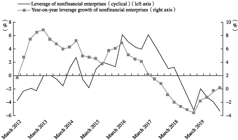
Cyclical Leverage Change of Nonfinancial Enterprises and Their Year-on-Year Leverage Growth
Note: This paper puts raw leverage data through HP filtering and gets the leverage ratio of nonfinancial enterprises (cyclical).
Source: Wind database.
Phenomenon 2: As the deleveraging policies were adopted, year-on-year growth of aggregate financing to the real economy (AFRE) (stock) and Li Keqiang index both fell in general. The year-on-year AFRE (stock) growth gradually declined from the peak in 2017 and echoed the leverage decrease of nonfinancial enterprises. Meanwhile, the drop of AFRE (stock) was consistent with the decrease of Li Keqiang index in reflection of economic vitality (Figure 2).

Year-on-Year Growth of AFRE (Stock) and Li Keqiang Index
Source: AFRE (stock) data is sourced from the People’s Bank of China and Li Keqiang index data from Wind database.
Phenomenon 3: Deleveraging policies represented by tight financial regulation promoted the size of shadow credit to turn from expansion to contraction. According to Figure 3, the actual size of shadow banking generally grew during 2012–2017 as driven by financial liberalization and absence of regulation, and then plunged after 2017 as financial regulation was tightened, leading to the AFRE adjustment at the same time.
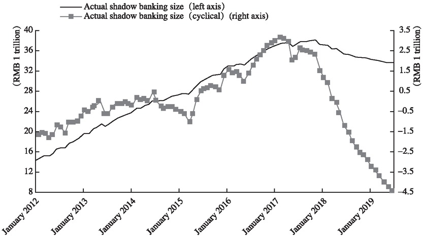
Actual Shadow Banking Size and the Cyclical Part
Note: This paper refers to Li (2019) to calculate the size of shadow banking in China at the liability end. The nominal shadow banking size after seasonal adjustment is divided by CPI to get the actual shadow banking size, which is subject to HP fi ltering to get the actual shadow banking size (cyclical). Source: The People’s Bank of China.
Phenomenon 4: Credit spread exhibited a “downward–upward” trend, and the number of bond defaults rose in general. Figure 4 shows that credit spread of 5-year medium-term notes (AAA) started a downward trend from 2012 to early 2016, but began surging as driven by deleveraging policies since August 2016. Similarly, in the context of financial deleveraging, due to credit contraction and narrowing financing channels, rigid redemption was broken. The number of corporate credit bond defaults rapidly climbed since 2016. [1]

Credit Spread and the Number of Bond Defaults
Note: In calculation of the number of bond defaults, this paper uses bonds in the status of “material breach”. Source: Wind database.
3 Theoretical Models
3.1 Representative Households
Representative households get access to labor-based wage income, which they use on consumption and bank savings. Household income for term t includes term-t risk-free securities At with a risk-free rate of return
3.2 Goods Sector
Goods sector uses capital Kt and labor Nt for production, and the output Yt is eventually used for household consumption and capital formation. Assume the production function of the goods sector has constant returns to scale and the production function equation is
3.3 Banks
At the end of term t, banks of perfect competition sell risk-free securities At+1 to the household sector and promise them risk-free rate of return
In the perfect competition market, in order to ensure that banks can pay households principal and interest of risk-free securities each term, the expected total return of bank loan portfolio should be equal to the opportunity cost of the risk-free securities that banks sell to households in any possible state. But in this paper, bank loans to each entrepreneur face overall risk and heterogeneity risk. In order to fulfill the previous condition, this paper refers to Bernanke et al. (1999), assuming that entrepreneurs are risk-neutral and each one is willing to undertake overall risk of loans and pay back “state-contingent” loans. Now, bank loans only suffer entrepreneur-related heterogeneity risk, and banks can eliminate such risk with large enough loan portfolios. This paper uses Ψt+1 to mean the expected total return of bank loan portfolios for term t+1, and bank budget constraint equation is:
3.4 Entrepreneurs
The economic activities of entrepreneur i include entrepreneur i buying capital K t +1 ( i ) for the new term from the capital goods sector at a price qt at the end of term t, its leasing capital to the goods sector at an interest rate of rt+1 at the beginning of term t+1, and its selling capital after depreciation back to the capital goods sector at the price qt+1 at the end of term t+1. The fund for entrepreneur i to purchase capital K t +1 ( i ) at the end of term t is sourced from its own term t-end net worth X t +1 ( i ) and loans B t +1 ( i ) from loan contracts signed with banks, and therefore term t-end credit determination equation of entrepreneur i can be shown as q t K t+1 ( i ) = X t+1 ( i ) + B t+1 ( i ) . Its term t-end leverage ratio is defined as the ratio between assets and net worth, i.e.
δ is capital depreciation. In reference to Bernanke et al. (1999), we assume ω can only be observed by entrepreneurs and is subject to the logarithmic normal distribution with a mean value of 1 and a standard deviation of σω, and the distribution function is recorded as F(ω).
To avoid the scenario where entrepreneurs of sufficient net worth of their own have no need of external financing, the paper refers to Bernanke et al. (1999) and includes the possibility of entrepreneur bankruptcy in the model to ensure entrepreneurs have to resort to banks for external financing. Define the survival rate of entrepreneurs as γ, which means at a term end, a 1-γ ratio of entrepreneurs exits from economy and meanwhile a 1-γ ratio of new ones enters the economy. The γ ratio of surviving entrepreneurs and the 1-γ ratio of newcomers both get access to transfer payment W e.
3.5 Banks and Standard Loan Contracts
In the model, banks provide entrepreneurs with loans by signing loan contracts. For specific arrangement, at the term t end, banks offer entrepreneur i a new term of loans for a mount of B t +1( i ) , and specify the “state-contingent” loan interest rate
When economy reaches the system equilibrium, we have
According to equation (1) and equation (2), we come to:
Given the definition of leverage ratio and equation (5), bank zero-profit equation is expressed as:
3.6 Contracts of Entrepreneurs
Entrepreneurs are risk-neutral and pursue the optimal goal of maximized expected net income. The expected net income function of entrepreneur i is
3.7 Capital Goods Sector
The capital goods sector of perfect competition uses the capital after depreciation (1−δ )Kt purchased from entrepreneurs and the investment It originated from the goods sector at the term t end to produce the new term of capital Kt +1 . We refer to Fernández-Villaverde (2010) and express the capital accumulation equation as:
3.8 Exogenous Shocks
The paper presumes that default costs follow the exogenous shock process:
Furthermore, the paper hopes to discuss response of economic individuals to the news of future default costs. By referring to Gunn and Johri (2013) and Gunn (2018), it divides exogenous shocks into unanticipated current shock and anticipatable shock, i.e.
3.9 Other Equations
Output of the goods sector is mainly used in consumption, investment and entrepreneurs’ loan default loss. The resource constraint equation is:
The equation for entrepreneurs’ net worth during equilibrium is:
To support the analysis, this paper defines term-t external finance premium as the ratio between entrepreneurs’ expected return on capital and risk-free interest rate, i.e.
4 Parameter Calibration
To analyze the dynamic changes of various macroeconomic variables under financial shocks, similar to the majority of previous studies, this paper resorts to previous literature, historical data or steady-state equations to identify the model parameters through calibration. Next, parameter value will be discussed one by one by sector (Table 1). Since one term in the model here corresponds to one quarter in reality, quarterly data is applied for parameter calibration.
Parameter Calibration
| Parameter | Meaning | Value |
|---|---|---|
| α | Share of capital | 0.5 |
| β | Discount factor | 0.994 |
| ξ | Disutility weight of labor | 6.7 |
| χ | Reciprocal of labor supply elasticity | 1 |
| δ | Capital depreciation | 0.025 |
| φ | Intensity of investment adjustment cost | 0.259 |
| γ | Survival rate of entrepreneurs | 0.98 |
| W e | Transfer payment of entrepreneurs | 0.005 |
| σω | Standard deviation of logarithmic value of heterogeneity shock | 0.25 |
| θ̅ | Steady-state value of default cost | 0.1 |
| ρ | Persistence parameter of financial shocks | 0.95 |
| σθ | Standard deviation of financial shocks | 1 |
Main parameters for the household sector include discount factor β, reciprocal of labor supply elasticity χ, and disutility weight of labor ξ. In the steady state, discount factor β depends on the level of risk-free interest rate. This paper finds after calculation that yield to maturity of one-year national debt was averaged at 2.58% during 2002–2019, and therefore sets the discount factor β at 0.994. Regarding labor supply elasticity, Wang and Wang (2010) pointed out the majority of studies selected the labor supply elasticity 1/χ at (0.15, 2). This paper refers to the setting of Christiano et al. (2014) and Li and Liu (2014) and selects the labor supply elasticity at 1. According to the prevailing practice, steady-state value N of hours of labor is set at 1/3; based on this value and the steady-state equation in equilibrium, disutility weight of labor ξ is further calibrated to 6.7.
The share of capital α in the production function of the goods sector is mostly valued 0.3~0.6 in the majority of studies. In reference to Wang and Tian (2014), Wu et al. (2011) and Lin et al. (2018), α is valued 0.5 here. Parameters of the capital goods sector include capital depreciation δ and intensity of investment adjustment cost φ. By referring to Chen and Gong (2006), Wang and Wang (2010) and Yan and Wang (2012), δ is set at 0.025. φ refers to the setting of Wang and Tian (2014) and Jin et al. (2017) and is valued 0.259.
Parameters of the entrepreneur sector include steady-state value of default cost
5 Intrinsic Mechanisms of Entrepreneurs’ Leverage Changes
As a primary factor in the model of this paper, default costs of the loan contracts between entrepreneurs and banks produce significant effects on macroeconomic variables. Before the impulse response analysis, this part will theoretically analyze the intrinsic mechanisms for the influence of default costs on entrepreneur leverage, and elaborate on the direct and indirect channels for such influence. First, according to equation (7) and the definition of external finance premium, we get the implicit expression of the entrepreneur leverage:
It’s revealed that the changes with entrepreneur leverage is subject to the joint influence of external finance premium, default costs and default threshold. In the conventional financial accelerator model, default cost is usually set as a fixed parameter, in which case external finance premium and default threshold are positively correlated, and entrepreneur leverage and default threshold are positively correlated (left in Figure 5). Under the classic financial accelerator mechanism, with default costs remaining constant, as external finance premium rises, default threshold climbs accordingly and entrepreneurs assume higher debts to expand size, driving up the leverage ratio as well.
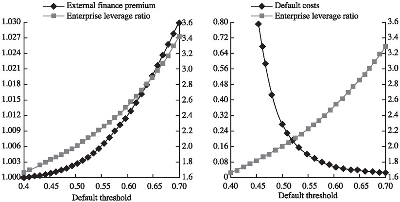
Connections of External Finance Premium, Enterprise Leverage Ratio and Default Threshold Note: Default costs are given on the left and external finance premium is given on the right.
In the model of this paper, default costs change under the influence of financial shocks. Changes with default costs may affect entrepreneur leverage through direct and indirect channels. On the one hand, the changes affect external finance premium and consequently indirectly affect the leverage through the financial accelerator. On the other hand, the changes produce direct influence over the leverage. Increase of default costs will directly drive up the leverage. It shows on the right of Figure 5 that when external finance premium remains constant, default costs and default threshold are negatively correlated, and entrepreneur leverage and default threshold are positively correlated. In this case, rising default costs will lead to lower default threshold and leverage.
In summary, when default costs are fixed, entrepreneur leverage and external finance premium change in the same direction; when external finance premium remains constant, the leverage and default costs alter in opposite directions. To explain the intrinsic mechanism for the influence of changing default costs on entrepreneur leverage, the cost changes will directly cause the leverage change on the one hand, and on the other, bring about changes with external finance premium and indirectly weaken the previous changing trend of leverage. The ultimate effects of default costs on leverage will depend on both direct and indirect effects.
6 Impulse Response Analysis
To explain the “expansion–contraction” fluctuations of Chinese macroeconomy between before and after practice of deleveraging policies, we firstly analyze the dynamic changes of all the macroeconomic variables under unanticipated financial shocks and explore the influence of actual default cost changes on macroeconomic variables. Secondly, we take into account effects of anticipated shocks and analyze the macroeconomic fluctuations caused by the anticipated changes of default costs in the circumstances of expectation realization and expectation reversal.
6.1 Unanticipated Shocks
We now analyze the changes with macroeconomic variables as a result of negative unanticipated financial shocks (default costs dropping). Figure 6 indicates that lower default costs increase the credit supply, push up the entrepreneur leverage, lower the credit spread, and also cause the output and investment to rise. [1] As the entrepreneur leverage L and risk-free interest rate Rd in the model are determined by the previous term, according to the bank zero-profit equation (6), the drop of default costs θ means the default threshold ϖ and return on capital Rk will first change in the current term of shocks. As anticipated bank return consists of the non-default loan value and the default loan value, decreased default costs mean that banks’ current non-default loan value falls and default threshold drops accordingly. The drop of default threshold is associated with the decrease of current credit spread spread [2] and the increase of entrepreneur net worth X (result of the equation (11)). Higher X indicates that entrepreneur demand for capital K rises correspondingly (entrepreneurs are the buyer of capital). According to equation (8), the capital goods sector will increase investment I, and the goods sector will raise output Y to satisfy the incremental investment (result of the equation (10)). The investment changes cause the capital price q to climb and further drive up the return on capital Rk (result of the equation (3)). According to equation (6), higher Rk will lead to lower default threshold and trigger the decrease of credit spread spread and the increase of entrepreneur net worth X. In the current term of shocks, therefore, changes with the default threshold ϖ, credit spread spread, and entrepreneur net worth X are subject to the joint influence of default costs and return on capital.
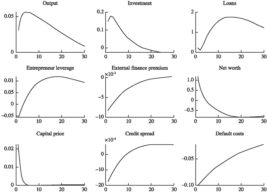
Impulse Response of Negative Financial Shocks (Default Costs Dropping)
Similarly, rise of the current entrepreneur net worth X will further drive up entrepreneur demand for capital K of the next term (the 2nd term), which will cause the capital goods sector to correspondingly increase the new-term investment I, the goods sector to correspondingly raise the new-term output Y, and the capital price q to keep climbing positively. This will drive return on capital Rk to grow continuously and further trigger lower default threshold ϖ for the new term, lower credit spread spread and higher entrepreneur net worth X. According to the entrepreneur credit determination equation (4), increase of the entrepreneur net worth X for the new term is sufficient to raise its loan demand, to which end banks need raise more funds, causing the risk-free interest rate Rd for the new term to rise. Households provide banks with more risk-free securities A, and according to equation (1), new-term loan B keeps expanding positively. In addition, according to the implicit expression of leverage equation (12), since the drop of default costs θ affects entrepreneur leverage L both directly and indirectly, under the dual effects, new-term entrepreneur leverage responds negatively, which sustains for only the first few terms, and afterwards the leverage keeps rising positively. This means the direct effects of default costs on entrepreneur leverage take a predominant position and lower default costs generally push up the entrepreneur leverage. In this paper, we understand the default cost changes caused by financial shocks as the actual default cost changes as a result of changing financial regulation policies in recent years. When regulation is relaxed, average default costs of economy in the model decline, leading to rise of entrepreneur leverage, expansion of loans and drop of credit spread; when regulation is tight, the average default costs rise, bringing about lower entrepreneur leverage, contracted loans and higher credit spread. The synchronous changes with leverage, credit spread, credit and other macroeconomic variables caused by the actual default cost changes can be verified by the economic changes of China in recent years (the second part in the paper).
6.2 Anticipated Shocks
Furthermore, we hope to analyze the response of the model to anticipated changes with default costs and pay close attention to the influence of decrease of the anticipated costs (presuming banks get the news of default cost decrease for the 10th term in the first term).
First, we look at the changes with various macroeconomic variables in the case of expectation realization (i.e. the news of default cost decrease proves to be correct), and closely follow the response of the economic variables before actual shocks occur. Figure 7 reflects that after the expectation is realized, investment and output continue to grow, loans keeps expanding positively, credit spread drops, and entrepreneur leverage positively rises. In the first to tenth term before actual shocks occur, lower anticipated default costs cause investment output and loans to expand positively and credit spread to drop negatively. Under the dual effects of default costs, entrepreneur leverage is briefly negative for the first few terms and then turns to climb positively under the predominant direct effect. In general, default costs show no alteration after the 10th term, but the solely expectation-driven model economy fluctuates in expansion.

Impulse Response under Expectation Realization
Next, we turn to the response of the economic variables during expectation reversal (i.e. the news of default cost decrease is not realized in the 10th term). According to Figure 8, compared with the 10th term, starting with the 11th, investment and output plunge after hitting the peak, credit spread surges, and entrepreneur leverage and loans gradually drop back. Regarding credit spread, since the news of actual default cost drop fails to materialize, compared with the 10th term, credit spread declines to the bottom and rapidly climbs to the highest point in the 11th. As to entrepreneur leverage, it keeps rising in the current term of actual news occurrence and both before and after that, and its changes relatively lag behind credit spread with the advent of the news. As the news fails to realize, starting with the 11th term, entrepreneurs will select new leverage ratio and default threshold, and Figure 8 indicates the positive response of leverage reaches the peak in the 11th term before gradually dropping back. In the case of expectation reversal, anticipated changes alone can drive the economy to fluctuate in “expansion–contraction”.
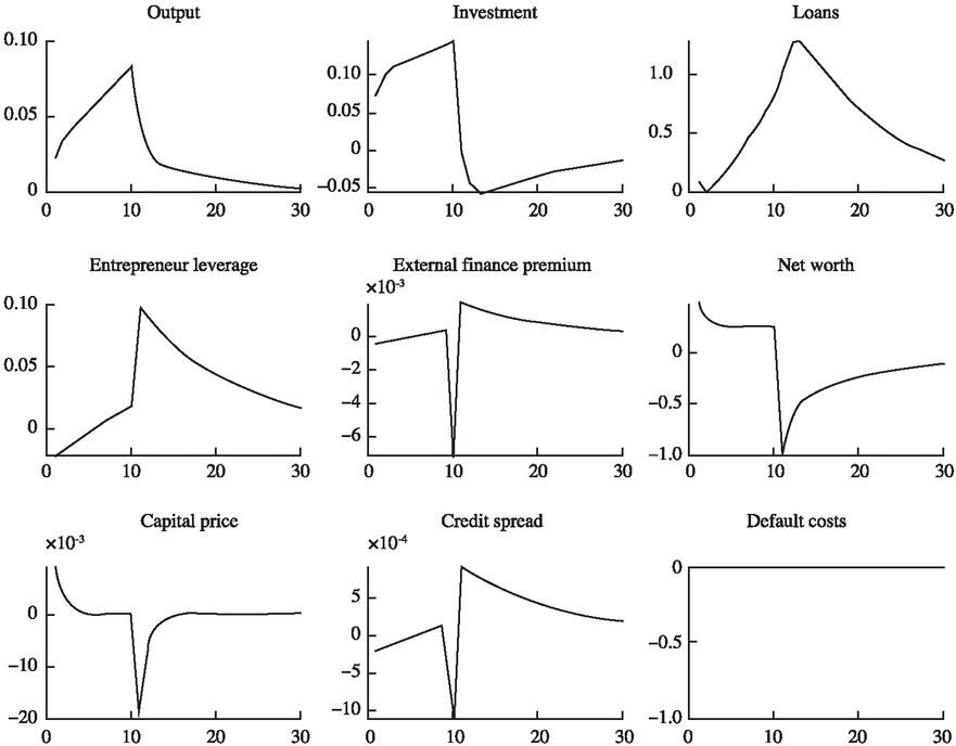
Impulse Response under Expectation Reversal
Based on the above-mentioned impulse response result, this paper believes that the changes with expectation dimensions of default costs can be used to explain China’s macroeconomic reality before and after the deleveraging policies were adopted. Prior to 2016, banks placed hope on the prosperity of the real estate market and the implicit guarantee from local government for city investment platforms and industries of high energy consumption, heavy pollution and overcapacity, and their favorable expectations for growing real estate market and implicit guarantee prompted banks’ expectation for declining default costs. Banks used shadow banking to introduce massive funds into the investment-limited industries, causing credit and leverage to rise and credit spread to drop, even though the real estate market didn’t change in any material way. Since the second half of 2016, however, central government put into effect a series of documents for fending off major risks and enhancing financial regulation. In the first quarter of 2017, CBRC issued seven documents intensively; CSRC, CIRC and industrial associations continued to launch various regulatory regulations and systems for financial rectification; the central bank included off-balance sheet wealth management into MPA assessment. Driven by the deleveraging policies, central government could reverse banks’ expectation for default costs by releasing signals of regulating real estate, breaking rigid repayment of implicit debts and changing the confidence level of local implicit guarantee, so as to attain the purpose of narrowing down economic credit and reducing leverage.
7 Conclusions and Inspirations
This paper constructs a financial business cycle model based on the financial accelerator theory, and uses financial shocks in reflection of changing default costs to describe the changes with deleveraging polices, giving reasonable explanations for the macroeconomic fluctuations before and after the deleveraging was practiced in the two perspectives of unanticipated and anticipated shocks. By analyzing the intrinsic mechanism of the model, it introduces the two effects of default costs on entrepreneur leverage. The decrease of default costs will directly drive up leverage on the one hand, and on the other hand, cause external finance premium to drop and indirectly bring down leverage through the financial accelerator mechanism. The eventual influence of default costs on entrepreneur leverage depends on the relative strength of the two effects. Furthermore, based on impulse response analysis, the paper explains that lower default costs will lead to higher investment and output, expanding loans, rising leverage and lower credit spread. On this account, the changes with unanticipated default costs can be used to describe the fluctuations of credit, leverage, credit spread and other major macroeconomic variables between before and after the deleveraging in recent years. When anticipated factors are added, the drop of anticipated default costs will cause investment, output and loans to surge, while all the changes occur before the default costs actually change. With expectation reversal taken into account, all the economic variables will fluctuate in opposite directions. Therefore, anticipated default cost changes alone can also trigger the “expansion–contraction” economic fluctuations, consistent with the recent macroeconomic fluctuations in the deleveraging context in China.
At present, as the deleveraging has evolved to the stage of stabilizing leverage, deleveraging policy measures are suggested to pay close attention to the following two areas. First, given that credit default events in Chinese bond market will turn regular in general, it’s necessary for government to highlight the warning effect of default costs, practice deleveraging at proper rhythm and with proper strength, promote enterprises to utilize leverage reasonably, and improve the rational awareness in the market for the default trend. Second, China’s macroeconomic fluctuations of “expansion–contraction” in recent years can be explained with the anticipated changes with default costs in a certain dimension. When issuing and practicing policies, government should attach importance to expectation management and especially to expectation guidance for financial institutions, and put into play the important role of the finance sector over deleveraging.
Funding statement: Supported by: “Study on the Chinese Macroeconomic Fluctuations in the DSGE Model Framework” (19FJLB002), a project supported by a grant from The National Social Science Fund of China; “Macroeconomic Risks, Anticipated Shock and Asset Pricing: Based on the DSGE Model” (2722020JX012), a project supported by the Fundamental Research Funds for the Central Universities (Interdisciplinary Innovation Research). The authors would like to thank the anonymous reviewers for their valuable comments and suggestions, and take sole responsibility for the paper.
References
Altman, E. (1984). A Further Empirical Investigation of the Bankruptcy Cost Question. The Journal of Finance 39(4), 1067–1089.10.1111/j.1540-6261.1984.tb03893.xSuche in Google Scholar
Beaudry, P., & Portier, F. (2006). Stock Prices, News, and Economic Fluctuations. American Economic Review 96(4), 1293–1307.10.3386/w10548Suche in Google Scholar
Bernanke, B., Gertler, M., & Gilchrist, S. (1999). The Financial Accelerator in a Quantitative Business Cycle Framework. Handbook of Macroeconomics 1, 1341–1393.10.3386/w6455Suche in Google Scholar
Chen, K., & Gong, L. (2006). Numerical Simulation for China Economy in a Sticky-Price Model. The Journal of Quantitative & Technical Economics (Shuliang Jingji Jishu Jingji Yanjiu) 8, 106–117.Suche in Google Scholar
Chen, K., Ren, J., & Zha, T. (2018). The Nexus of Monetary Policy and Shadow Banking in China. American Economic Review 108(12), 3891–3936.10.3386/w23377Suche in Google Scholar
Christiano, L., Motto, R., & Rostagno, M. (2014). Risk Shocks. American Economic Review 104(1), 27–65.10.3386/w18682Suche in Google Scholar
Cui, G. (2006). Asset Price, Financial Accelerator, and Macroeconomic Stabilization. The Journal of World Economy (Shijie Jingji) 29(11), 59–69.Suche in Google Scholar
Du, Q., & Gong, L. (2005). The RBC Model with the “Financial Accelerator”. Journal of Financial Research (Jinrong Yanjiu) 14(4), 16–30.Suche in Google Scholar
Fernández-Villaverde, J. (2010). Fiscal Policy in a Model with Financial Frictions. American Economic Review 100(2), 35–40.10.1257/aer.100.2.35Suche in Google Scholar
Fuentes-Albero, C. (2019). Financial Frictions, Financial Shocks, and Aggregate Volatility. Journal of Money, Credit and Banking 51(6), 1581–1621.10.1111/jmcb.12554Suche in Google Scholar
Gunn, C. (2018). Overaccumulation, Interest, and Prices. Journal of Money, Credit and Banking 50(2-3), 479–511.10.1111/jmcb.12468Suche in Google Scholar
Gunn, C., & Johri, A. (2013). An Expectations-Driven Interpretation of the “Great Recession”. Journal of Monetary Economics 60(4), 391–407.10.1016/j.jmoneco.2013.04.003Suche in Google Scholar
Jin, P., Wang, Y., & Zhang, L. (2017). Financial Friction and Leverage Governance in Perspective of Maintaining Stable Growth. Journal of Financial Research (Jinrong Yanjiu) 4, 78–94.Suche in Google Scholar
Levin, A., Natalucci, F., & Zakrajsek, E. (2004). The Magnitude and Cyclical Behavior of Financial Market Frictions. Finance and Economics Discussion Series (FEDS) Working Paper, 70.10.17016/FEDS.2004.70Suche in Google Scholar
Li, L., & Liu, Y. (2014). Variation of Economic Fluctuations and Reconstruction of China’s Macroeconomic Policy Framework. Management World (Guanli Shijie) 12, 38–50.Suche in Google Scholar
Li, T., Zhang, Y., & Zhang, H. (2017). Research on Macro-Prudential Policy Rules and the Conduction Path. Management World (Guanli Shijie) 10, 20–35.Suche in Google Scholar
Li, W. (2019). Economics of China’s Shadow Banking: Definition, Composition and Measurement. Journal of Financial Research (Jinrong Yanjiu) 3, 53–73.Suche in Google Scholar
Lin, B., Wang, D., & Chen, S. (2018). Heterogeneous Efficiency Firms, Resource Reallocation Mechanism of Financial Frictions and Economic Fluctuations. Journal of Financial Research (Jinrong Yanjiu) 8, 17–32.Suche in Google Scholar
Liu, S., Wang, Z., Cheng, Y., & Xu, W. (2018). Reducing Business Costs: Survey and Analysis in 2018. Public Finance Research (Caizheng Yanjiu) 10, 2–24.Suche in Google Scholar
Liu, Y., & Wang, L. (2018). Endogenous Leverage Threshold, Financial Accelerator and Economic Fluctuation: A DSGE Model. South China Journal of Economics (Nanfang Jingji) 12, 57–77.Suche in Google Scholar
Milani, F., & Treadwell, J. (2012). The Effects of Monetary Policy “News” and “Surprises”. Journal of Money, Credit and Banking 44(8), 1667–1692.10.1111/j.1538-4616.2012.00549.xSuche in Google Scholar
Wang, G., & Tian, G. (2014). Financial Shocks and Chinese Business Cycles. Economic Research Journal (Jingji Yanjiu) 3, 20–34.Suche in Google Scholar
Wang, J., & Wang, W. (2010). Market of Imperfect Competition, Technology Shocks and China’s Labor Employment: In a Dynamic New Keynesianism Perspective. Management World (Guanli Shijie) 1, 23–35.Suche in Google Scholar
Wu, H., Xu, Z., Hu, Y., & Yan, P. (2011). Fiscal Policy under the News Shock and the Macro Influence. Management World (Guanli Shijie) 9, 26–39.Suche in Google Scholar
Yan, L., & Wang, Y. (2012). Financial Development, Financial Market Shocks and Economic Fluctuations: A DSGE-Based Analysis. Journal of Financial Research (Jinrong Yanjiu) 12, 82–95.Suche in Google Scholar
Zhao, M., Yu, L., & Zhang, H. (2016). Financial Frictions, Default Shocks and Chinese Economic Fluctuations. Journal of Central University of Finance & Economics (Zhongyang Caijing Daxue Xuebao) 11, 76–83.Suche in Google Scholar
Zhao, Z., Yu, Z., & Liu, M. (2007). Does the Financial Accelerator Effect Exist in China? Economic Research Journal (Jingji Yanjiu) 6, 27–38.Suche in Google Scholar
Zhou, X., Li, H., Li, K., & Su, N. (2017). Soft Budget Constraint, Financing Premium and Leverage: Micro-Mechanism and Economic Effects of the Supply-Side Structural Reform. Economic Research Journal (Jingji Yanjiu) 52(10), 53–66.Suche in Google Scholar
Zhuang, Z., Cui, X., Gong, L., & Zou, H. (2012). Expectations and Business Cycle: Can News Shocks Be a Major Source of China’s Economic Fluctuations? Economic Research Journal (Jingji Yanjiu) 6, 46–59.Suche in Google Scholar
© 2022 Ziguan Zhuang, Jinbu Zou, Dingming Liu, published by De Gruyter
This work is licensed under the Creative Commons Attribution 4.0 International License.
Artikel in diesem Heft
- Theoretical Logic and Empirical Facts of Consumption Structure Upgrade and Domestic Value Chain Circulation under the New Development Pattern
- Financial Shocks, Deleveraging and Macroeconomic Fluctuations in China
- Local Government Borrowing’s Expansionary Monetary Effect and Its Policy Synergy
- Distance Puzzle: An Explanation from Global Value Chain Perspective
- Exchange Rate Change, Factor Market Distortion and Company Performance
- Policy Innovation Diffusion and PPP Spatial Distribution