
Distance Puzzle: An Explanation from Global Value Chain Perspective
-
Yuwan Duan


Abstract
Theoretically, along with the technology progress and infrastructure improvement, geographical distance should have a diminishing effect on international trade over time. However, the empirical studies failed to deliver consistent empirical support for it. This result is known as “distance puzzle”. In this paper, we propose that the intermediate goods across borders caused by global value chain (GVC) could be an important explanation for the “distance puzzle”. We firstly build a Ricardian model with two stages of production, by which the trade elasticity under the framework of traditional trade and GVC trade are derived and compared, to theoretically explain why the GVC will result in the “distance puzzle”. Then we empirically investigate the effect of distance and cross-border times on bilateral gross trade and value-added trade over time. After controlling the influence of the GVC, we observe a diminishing elasticity of distance over time, and prove that the GVC can explain the “distance puzzle”. The further heterogeneous analysis and robustness tests confirm our empirical results.
1 Introduction
International trade serves a powerful engine driving economies across the globe. “Openness brings progress, while self-exclusion leaves one behind,” as President Xi Jinping noted at the 19th National Congress of the Communist Party of China. Opening up is the path China must take to achieve prosperity and development in line with economic developments at home and abroad. Factors influencing trade remain as important contents in related studies as always. Geographical distance is believed to be a crucial a trade cost (Head and Mayer, 2014). Along with the technology progress and infrastructure improvement, geographical distance is supposed to have a diminishing effect on international trade over time. However, the empirical studies fail to deliver consistent empirical support for it, but with findings of an increasing effect over time (Brun et al., 2005; Coe et al., 2007). This paradox is known as “distance puzzle” (Cairncross, 1997). Previous studies partially explained the “distance puzzle” from omitted variables, no-trade response, etc. (Brun et al., 2005; Coe et al., 2007). In this paper, we propose that the GVC could be an important explanation for the “distance puzzle” since the 1990s as a supplementary prospective to previous efforts.
The GVC development is a dominant feature of the world economy. The 30 years of IT progress and increasingly detailed division of labor which enables different stages of production to be finished in various countries and no longer in a single one. Economies all over the world are brought together with prospects for growth, development and employment. According to the World Bank report, 50% of world trade now occurs through GVCs which are vital to global economic development. Rapid progress of GVCs has restructured the world economy and changed global trade, investment and production ties, while new challenges are posed to traditional trade theories and empirical studies and also to the making of trade policies. In this paper, the international trade paradox “distance puzzle” is explained with controlling for the influence of the GVC.
Through GVCs, products experience multiple stages of production distributed around the world. As cross-border times increase with the number of stages of production, the international division of labor and trade volume become more sensitive to changes in trade costs (Antràs and de Gortari, 2020). That being said, the actual volume of trade will be overestimated as a result of double counting as products cross national borders many times; For countries at shorter distances, their volume of trade is more sensitive to changes of distance, because the lower their trade costs are, the more detailed the international division of labor is, and the more cross-border times of intermediate goods, the more double counting into gross trade accounting will be. In other words, GVCs allow for larger trade between closer countries and then result in a greater elasticity of distance. This effect grows as the international division of labor deepens, and thereby an increasing elasticity of distance is seen over time with a more detailed division of labor when countries are closer to each other.
This paper will theoretically and empirically prove that the GVC is an important explanation for the “distance puzzle” after 1990s. We first build a Ricardian model with multiple stages of production, by which the elasticities of distance are compared under the traditional trade (without GVCs) and GVC trade, to theoretically explain that the GVC will increase the effect of distance on trade. Then the theory is empirically investigated using cross-country panel data of 42 economies in 2000-2014 and the Gravity Model. After controlling the influence of the GVC, we observe a diminishing elasticity of distance over time, and prove that the GVC can explain the “distance puzzle”. We also look into how the GVC influences the elasticity of distance, and the further heterogeneous analysis and robustness tests confirm our empirical results. Explaining the paradox “distance puzzle” from the GVC perspective is an important contribution to international trade studies and lays a foundation for re-examining international trade theories and experiences in GVCs. It is of practical significance to interpret trade growth and efficiently promote “openness for development” in the new era.
The rest of this paper is arranged as follows. The second part is literature review; the third part builds a Ricardian model with multiple stages of production to theoretically explain the effect of GVCs on the elasticity of distance; the fourth part introduces the measurement model and data; the fifth part is empirical analysis and robustness test; the final part is the conclusion.
2 Literature Review
This paper closely relates to the literature on “distance puzzle” and GVCs. Previous studies of “distance puzzle” have mostly applied the Gravity Model for analyzing the effect of distance on trade volume and its changes over time. Disdier and Head (2008) conducted a “meta-analysis” of empirical findings from 103 economic literatures about the effect of distance on trade, and concluded that the elasticity of distance in most studies did not diminish over time, but they offered no explanation for the “distance puzzle”.
The existing literature have contributed three explanations for how the “distance puzzle” appears. First, improperly designed models and the deviation of omitted variables resulted in an inability to precisely estimate the elasticity of distance (Brun et al., 2005; Carrère and Schiff, 2005). Using data from 130 economies in 1962-1996, Brun et al. (2005) added the infrastructure quality, the oil price index and the proportion of primary product exports in gross exports to their model, and observed a diminishing effect of distance on trade on a yearly basis. Second, the trade volume measurement affected estimating the elasticity of distance. Felbermayr and Kohler (2006) took that the omission of no-trade volume might affect estimating the elasticity of distance, as they used Tobit model to regress the no-trade sample and found it feasible to explain the “distance puzzle”. Larch et al. (2016) and Silva and Tenreyro (2006) considered that no-trade volume should be handled with the Poisson Pseudo Maximum Likelihood (PPML). The “distance puzzle” could be observed using Ordinary Least Square (OLS), as noted by Bosquet and Boulhol (2015), and when applied with PPML estimation, it could be alleviated but still would not disappear completely. Third, changes in the composition of trading nations and products led to the “distance puzzle”. Carrère et al. (2013) found that the “distance puzzle” existed only in trade among low-income countries and nothing about it among middle-and high-income countries by using data of 176 economies in 1970-2006 for regression. Lin and Sim (2012) noted that countries at longer distances witnessed more increases of trade extensive margin and relatively slow growth of trade volume, while closer countries gained more intensive marginal increases and seemingly, the effect of distance on trade appeared to grow on a yearly basis. The sample for estimating the “distance puzzle” should include both domestic and international trade, as held by Yotov (2012), whose estimation results using OLS and PPML revealed a fall by 28% and 37% in the elasticity of distance on trade in 1965-2005 respectively. Generally, many explanations for the “distance puzzle” were covered by previous studies, but the sample period was early and few studies targeted at recent years’ “distance puzzle”. Factors influencing trade and the elasticity of distance continue to evolve as the world trade and economy are ever-changing. In this paper, we will investigate and explain the “distance puzzle” since the 21st century.
Emerging at the end of the 20th century and rising rapidly in the 21st century to be a dominant feature of today’s global economy, GVCs are formed with countries and regions engaging in different stages of production of the same product. Currently, research ideas and approaches concerning GVCs have spread to wide fields related to economics, and become a research hotspot of economics. Measuring GVCs is a research core in recent years. One of the tasks is to restore the real picture of international trade under economic globalization and better reveal the benefits of nations in global trade. By its unique advantages, the input-output model has become mainstream for tracking GVCs, based on which a variety of studies were systematically conducted at the national or industry level. The vertical specialization (VS) rate was defined by Hummels et al. (2001) and Yi (2003) as the imports per unit of exports and measures the vertical division of labor of a nation. Johnson and Noguera (2012) proposed an approach to calculating the value added of bilateral trade at home and abroad based on the input-output model, confirmed the large difference in the bilateral trade balance measured by gross trade and value-added trade, and argued that value-added trade could better reveal the trade benefits of both sides (Timmer et al., 2013). Their calculation of value-added trade in 1970-2010 (2012b) found a yearly decreasing ratio of value-added trade to gross trade, meaning the double counting was getting worse over time. Koopman et al. (2014) decomposed gross exports into value-added exports, returned domestic value-added, foreign value-added, and double counting of intermediate goods (KWW method) according to value flows. Wang et al. (2017a; 2017b) set forth indicators measuring the participation of GVCs, the length of the production chain and cross-border times. What’s more, many studies specially worked on China’s position through GVCs as it has been called “The World’s Factory” (Kee and Tang, 2016; Zhang et al., 2013; Pan and Li, 2018; Shao et al., 2018; Hong and Shang, 2018).
In short, the “distance puzzle” and GVCs are both important research issues of international trade and yet no studies make a close connection of them. This paper is here to make up for this and explains the “distance puzzle” from the GVC perspective. We firstly build a Ricardian model, by which the modes of production of traditional trade (without GVCs) and GVC trade are compared, to theoretically explain how the GVC will influence the elasticity of distance. Then the GVC’s effect on the elasticity of distance and its dynamics is investigated using cross-country panel data in 2000-2014.
3 Theoretical Model
Referring to the theoretical model framework of Yi (2010), we build a Ricardian model with multiple stages of production, based on which the elasticity of distance in GVC trade and traditional trade is derived respectively, to theoretically explain why the GVC will result in the “distance puzzle”.
3.1 Model Setting
For simplicity, we assume that the world consists of two symmetrical parts—home country and foreign country. The production or consumption activities in home country and foreign country are expressed by superscripts H and F respectively. Both countries produce the continuous product z ∈[0,1] involving two stages of production. The first stage produces intermediate goods and the second produces final goods for household consumption with intermediate goods. Here we take home country’s production as an example. In the first stage when manufacturers use intermediate input and labor to produce intermediate goods, the Cobb-Douglas production function is as follows:
where
where TH is a constant representing the home country’s average productivity; When the shape parameter θ is given, the larger TH, the higher the average productivity. θ (θ > 0) represents the dispersion of productivity among different products z. The larger θ, the smaller the dispersion of productivity. In international trade, TH represents a nation’s absolute advantages and θ determines its comparative advantages over different products (Caliendo and Parro, 2015).
The inputs in the second stage include labor and the first-stage outputs, and the production function is as follows:
where
The form of the utility function of representative consumers at home and abroad is the same; We take home country’s consumers as the example, and the utility function is as follows:
where cH (z) is the consumption of product z by home country’s residents; Residents’ income comes from wages, and the consumption meets the budget constraint as follows:
where wH is home country’s wage level, lH is home country’s population, and pH(z) is the price of final goods z; Equation (4) means that consumers’ consumption of different products z accounts for the same proportion of gross consumption.
We distinguish between traditional trade (without the GVC division of labor) and GVC trade, and compare the effect of distance on trade in these two scenarios. To simplify the model, assumptions are made based on the classical theory of international trade (Dornbusch et al., 1977; Caliendo and Parro, 2015): (1) The product market is a perfectly competitive market; (2) There is only distance cost d(d≥0) for cross-border trade, no border costs such as tariffs and zero distance cost in domestic trade; (3) Labor flows freely at home but cannot cross national borders; This suggests the same wage level within a nation; (4) Trade is balanced in each country; (5) There is no difference in quality of the same product z between countries.
3.2 Traditional Trade
When we first assume no GVC production and only one stage of production for product z, there is only final goods trade and no intermediate goods trade. This is called “traditional trade”. Then the production function of home country’s product z is as follows:
where lH (z) and M H (z) are the labor input and the raw material input respectively, and α is the proportion of raw material input to production costs. The productivity of home country to foreign country is defined as
We put product z in order of relative productivity Ar (z) from large to small according to the method of Dornbusch et al. (1977). The smaller z is, the higher home country’s relative productivity is and the lower production costs are. In international division of labor, the home country prefers the production of Ar (z) . We may use pH (z) and pF (z) to express the prices of home-produced and foreign-produced product z, respectively; wH and wF are the wages in home country and foreign country respectively; and PH and PF are the raw materials prices in home country and foreign country respectively. In a completely competitive market, it is known by the conditions for business profit maximization that:
where
We further determine the cut-off point for international division of labor as zH, while assuming that for any product z, each country always buys from those with the lowest prices. In this way, when
To exclude the effect of factors other than distance on trade volume, we adopt Yi (2010)’s assumption that home and foreign wages, average productivity and intermediate goods prices are the same. [1] This eliminates the absolute advantages of home production, but the productivity of different products is different. Two countries have different comparative advantages over different products. Bringing the equation (7) into equation (9) to obtain a cut-off point for production zH:
When z ∈[0, zH ] , the price of home products is lower than that of foreign products sold in home country, and home country will produce product z, otherwise it will import product z ∈[zH ,1] from foreign country. According to equation (10), the distance cost plays a decisive role in the cut-off point for international division of labor. The lower the distance cost d is, the smaller zH is, and the higher the import ratio. Home imports of foreign products are:
Home consumption is:
Ratio of home imports to home consumption of products (hereinafter referred to as domestic consumption):
Equation (13) reflects the effect of distance on trade, indicating that the elasticity of distance is the shape parameter of productivity distribution θ.
3.3 GVC Production
A typical feature of GVC production is the intermediate goods trade. In this mode of production, a country can outsource a certain stage of production to other economies. It is assumed that the first-stage production is finished only in final consumers and the second-stage can be outsourced to other economies. That is to say, if home country is the final consumer of product z, the first-stage production of z is finished only in home country; The second-stage production can be finished in home country or outsourced to foreign country. We use the superscript HH to express that two stages of production are finished in home country and HF to indicate that the first-stage production is finished in home country and the second-stage in foreign country.
The production functions of the first and second stages are shown in equations (1) and (3), respectively. The production function in HH mode will be obtained by taking equation (1) into equation (3):
The production function in HF mode is as follows:
The production prices for product z in HH mode and HF mode are as follows:
where
Consumers in each country buy product z from those with the lowest prices. The relative productivity of HH and HF modes is
Assuming that home country and foreign country are equal in the average productivity and wages, the cut-off point will be calculated by equation (18):
Home country’s resident income is
In the same way, foreign country can also choose to outsource the second stage of production to other economies (FH mode) or finish it by itself (FF mode). The production cut-off point
When comparing GVC trade and traditional trade, the elasticity of distance has increased from the θ to θ (1+α 2 ) . It reveals that the effect of distance on international trade is enhanced by the GVC division of labor, and is stronger than that of traditional trade.
In fact, (1+α 2 ) represents the average cross-border times between home country and foreign country in the midst of production and trade. In the GVC mode, home country’s imports of final goods from foreign country are
When production is further refined, more stages of production can be outsourced to other economies, cross-border times will increase, and the effect coefficient of distance on trade will be larger. As international division of labor continues to be refined over time, the elasticity of distance will increase to result in the “distance puzzle”.
3.4 Value-Added Trade in GVC Production
Compared with traditional trade, there are two explanations for changes in home country’s international trade volume through GVCs according to the previous theoretical analysis: one is the double counting of intermediate goods. In the above mode, the value of first-stage goods
If the double counting is removed from gross trade accounting, will the elasticity of distance in GVC trade be closer to that of traditional trade? Value-added trade removed the double counting from gross trade, and it was considered to be a true manifestation of a nation’s trade (Johnson and Noguera, 2012; Timmer et al., 2013). Then further analysis of distance on value-added trade is conducted. According to the definition of Johnson and Noguera (2012), value-added imports (V AB) of country A from country B mean the value added of country B that is fully brought by country B to meet the final demand of country A.
In traditional trade, a nation’s products are completely finished by itself, and its gross export value is its value added. In this case, the gross trade accounting and value-added trade accounting are equal. Therefore, equation (13) is also applicable to value-added trade, and the elasticity of distance of value-added trade is still θ.
In GVC trade, V HF is the value-added imports from foreign country. The domestic consumption of final goods is
The elasticity of distance under value-added trade is obtained by taking the natural logarithms on both sides of equation (21) and deriving ln(1+ d) :
The distance under value-added trade has less effect on trade than θ (1+α 2 ) under gross trade. Value-added trade excludes the double counting from gross trade, and to some extent alleviates the effect of cross-border production on the elasticity of distance. Meanwhile, the elasticity of distance in value-added trade is larger than θ, i.e., it is greater than that in traditional trade; This reveals the impossibility to prevent GVC from magnifying the effect of distance on trade even if the double counting is excluded from gross trade.
4 Measurement Model and Data
4.1 Measurement Equation and Variable Description
By the Gravity Model, gross trade data and value-added trade data are used to analyze the effect of distance on trade and its dynamics over time with equations (23)-(25) for regression. Equation (23) is the gross trade regression model, i.e., the classic gravity model of trade in the literature, where the dependent variable is the log of bilateral gross trade. Equation (24) controls the cross-border times of bilateral trade goods based on equation (23). According to equation (20), in GVC trade, the effect of distance on trade equals to the cross-border times multiplied by the elasticity of distance in traditional trade, so we put the product of cross-border times and distance into the regression equation. The product’s coefficient—the elasticity of distance after controlling the influence of the GVC—is a new variable measuring distance in GVC trade. It takes into account the cross-border times and measures the actual “travel” distance of trade goods. Equation (25) replaces the dependent variable with value-added trade on the basis of equation (24) to find out whether the exclusion of double counting from gross trade will influence the elasticity of distance.
In the above equation, i and j represent country i and country j; and t indicates the year. GTijt represents gross exports from country i to country j in t year. VATijt represents value-added imports of country j from country i in t year. distwij is the core variable representing the distance between country i and country j. Dt is a set of year dummy variables.
Variables Related to the Gravity Model
| Variable | Description | Unit | Observed value | Average value | Standard error | Minimum | Maximum |
|---|---|---|---|---|---|---|---|
| CBijt | Cross-border times | - | 25830 | 1.54 | 0.30 | 1.01 | 2.58 |
| lndistwij | Logarithm of distance | km | 1722 | 8.05 | 1.07 | 5.08 | 9.81 |
| lnVATij | Logarithm added trade of value- | Million USD | 25830 | 6.11 | 2.19 | -1.47 | 16.58 |
| lnGTijt | Gross trade logarithm | Million USD | 25830 | 6.29 | 2.40 | -3.54 | 17.19 |
| contigij | Is border? there a common | variable [0,1] | 1722 | 0.06 | 0.24 | 0.00 | 1.00 |
| comlang_offij | Is language? there a common | variable [0,1] | 1722 | 0.05 | 0.22 | 0.00 | 1.00 |
| fta_wtoijt | Is RTA? it within the same | variable [0,1] | 25830 | 0.51 | 0.50 | 0.00 | 1.00 |
| colij | Was relationship? there a colonial | variable [0,1] | 1722 | 0.02 | 0.13 | 0.00 | 1.00 |
| tdiff ij | Jet lag | Hour | 1722 | 3.63 | 3.42 | 0.00 | 11.58 |
| popit | Population or importer of exporter | Million persons | 630 | 101.61 | 263.26 | 0.38 | 1364.27 |
| euit | Is the importer or exporter a member of the EU? | [0,1] variable | 630 | 0.55 | 0.50 | 0.00 | 1.00 |
| comcurijt | Is currency? there a common | variable [0,1] | 25830 | 0.11 | 0.31 | 0.00 | 1.00 |
| comreligij | Is religion? there a common | variable [0,1] | 1722 | 0.20 | 0.27 | 0.00 | 0.98 |
| lngdpcapit | Logarithm of per-capita GDP of exporter or importer | USD/Person | 630 | 9.79 | 1.06 | 6.13 | 11.67 |
Note: For logarithmic variables, the variable unit means its unit before the logarithm is taken.
The international input-output model is applied to calculate value-added imports and average cross-border times. The value-added imports of country j from country i refer to the value added of country i generated by country i to meet the final demand of country j. That is:
where vi is the row vector of each industry’s value-added coefficient in country i; fkj is the column vector of final goods imports of country j from country k. B is the Leontief inverse matrix, and its sub-matrix Bik is the outputs of each industry from country i that are completely consumed for producing 1 unit of final goods of each industry in country k.
The method of Wang et al. (2017b) is used to calculate the average cross-border times of country i exports to country j: [1]
where Lii is domestic Leontief inverse matrix of country i. eij is the column vector of gross exports from country i to country j. The denominator in equation (27) expresses the value added of country i embodied in gross exports of country i to country j; The numerator represents the total cross-border times of the value added in gross exports from country i to country j.
4.2 Data Source
Trade data are mainly from the World Input-Output Database (WIOD, 2016) involving 43 economies from 2000 to 2014. [2] Equations (26) and (27) are used to measure bilateral cross-border times and value-added trade. Distance data are from Mayer and Zignago (2011) who calculated the average distance between two countries by weighting the proportion of the population of each city nationwide, with account of the effect of population distribution on trade. The introduction and descriptive statistics of variables are shown in Table 1, and the data are from CEPII database. [1]
5 Empirical Analysis
5.1 Benchmarking Regression
5.1.1 Basic Regression Results
The regression results based on equations (23)-(25) are shown in Table 2. We first used the gross trade regression model (23) to test the “distance puzzle”. In view of only 40 more economies in the WIOD database, we tested the “distance puzzle” with a more complete sample from the UN COMTRADE database covering all product trade data of 220 economies in 1995-2014. The regression results are shown in column (1) of Table 2. The elasticity of distance of gross trade fluctuated continuously from 1995 to 2014, but generally it was increasing to show the “distance puzzle”, which was consistent with the existing literature (Carrère and Schiff , 2005; Coe et al., 2007; Disdier and Head, 2008). Column (2) of Table 2 shows the gross trade regression results using WIOD data, with the elasticity of distance increasing from 1.379 in 2000 to 1.430 in 2014. Column (4) shows the regression results based on equation (24). The border crossings of trade goods through GVCs were included to tell the effect of GVCs on the elasticity of distance. After controlling the influence of the GVC, the “distance puzzle” disappeared, and the elasticity of distance experienced a slow fall from 0.464 in 2000 to 0.424 in 2014; The results verify that the GVC is an important explanation for the “distance puzzle”. While comparing the results in column (4) and column (2), after the influence of the GVC was controlled, the elasticity of distance decreased significantly, which was consistent with the above theoretical model findings. The results are shown in column (6) of Table 2 after a further exclusion of double counting from gross trade accounting and a regression with value-added trade as the dependent variable. The elasticity of distance of value-added trade was shown to be smaller than that of gross trade, and the equation (22) was verified. With addition of cross-border times, the regression results of value-added trade and gross trade are similar temporally with a diminishing elasticity of distance, and the “distance puzzle” disappeared.
Primary Regression Results
| Variable | Gross trade regression (full sample) | Gross trade regression (without cross-border times) | Gross trade regression (with cross-border times) | Value-add trade regression (with cross-border times) | |||
|---|---|---|---|---|---|---|---|
| (1) | (2) | (3) | (4) | (5) | (6) | (7) | |
| OLS | OLS | PPML | OLS | PPML | OLS | PPML | |
| -1.431*** (0.024) | - | - | - | - | - | - | |
| -1.221*** (0.028) | - | - | - | - | - | - | |
| -1.353*** (0.024) | - | - | - | - | - | - | |
| -1.416*** (0.022) | - | - | - | - | - | - | |
| -1.437*** (0.021) | - | - | - | - | - | - | |
| -1.545*** (0.021) | -1.379*** (0.028) | -0.218*** (0.005) | -0.464*** (0.004) | -0.097*** (0.001) | -0.271*** (0.003) | -0.056*** (0.001) | |
| -1.544*** (0.021) | -1.386*** (0.028) | -0.220*** (0.005) | -0.467*** (0.004) | -0.098*** (0.001) | -0.274*** (0.003) | -0.057*** (0.001) | |
| -1.551*** (0.021) | -1.385*** (0.027) | -0.219*** (0.005) | -0.466*** (0.004) | -0.096*** (0.001) | -0.274*** (0.004) | -0.056*** (0.001) | |
| -1.581*** (0.021) | -1.383*** (0.027) | -0.216*** (0.005) | -0.457*** (0.004) | -0.092*** (0.001) | -0.271*** (0.004) | -0.054*** (0.001) | |
| -1.588*** (0.021) | -1.346*** (0.027) | -0.200*** (0.005) | -0.446*** (0.004) | -0.085*** (0.001) | -0.260*** (0.003) | -0.049*** (0.001) | |
| -1.602*** (0.020) | -1.358*** (0.027) | -0.202*** (0.005) | -0.438*** (0.004) | -0.082*** (0.001) | -0.255*** (0.003) | -0.047*** (0.001) | |
| -1.584*** (0.020) | -1.378*** (0.027) | -0.204*** (0.005) | -0.428*** (0.004) | -0.078*** (0.001) | -0.249*** (0.003) | -0.045*** (0.001) | |
| -1.595*** (0.020) | -1.380*** (0.027) | -0.202*** (0.005) | -0.424*** (0.004) | -0.076*** (0.001) | -0.240*** (0.003) | -0.042*** (0.001) | |
| -1.620*** (0.020) | -1.365*** (0.027) | -0.199*** (0.005) | -0.417*** (0.004) | -0.073*** (0.001) | -0.235*** (0.003) | -0.041*** (0.001) | |
| -1.632*** (0.021) | -1.384*** (0.027) | -0.204*** (0.005) | -0.436*** (0.004) | -0.079*** (0.001) | -0.254*** (0.003) | -0.045*** (0.001) | |
| -1.622*** (0.020) | -1.399*** (0.027) | -0.207*** (0.005) | -0.419*** (0.003) | -0.075*** (0.001) | -0.240*** (0.003) | -0.042*** (0.001) | |
| -1.638*** (0.021) | -1.396*** (0.027) | -0.206*** (0.005) | -0.410*** (0.003) | -0.072*** (0.001) | -0.232*** (0.003) | -0.04*** (0.001) | |
| -1.626*** (0.021) | -1.417*** (0.027) | -0.210*** (0.005) | -0.417*** (0.004) | -0.073*** (0.001) | -0.237*** (0.003) | -0.041*** (0.001) | |
| -1.649*** (0.021) | -1.411*** (0.027) | -0.208*** (0.005) | -0.418*** (0.004) | -0.073*** (0.001) | -0.238*** (0.003) | -0.045*** (0.001) | |
| -1.612*** (0.021) | -1.430*** (0.028) | -0.210*** (0.005) | -0.424*** (0.004) | -0.074*** (0.001) | -0.241*** (0.003) | -0.042*** (0.001) | |
| Observed Value | 381907 | 25830 | 25830 | 25830 | 25830 | 25830 | 25830 |
| R2 | 0.741 | 0.885 | 0.976 | 0.979 | |||
Note: *, * * and * * * indicate significance at the 10%, 5% and 1% levels, respectively, and the values in brackets are robust standard errors. All regressions contained the control variables listed in Table 1, which were not reported for page space and were available on request. The fixed effects of time, importers, exporters were also controlled. The same goes for the following table.
5.1.2 Robustness Tests for Benchmarking Regression
Avoiding the effect of no-trade volume, we used PPML for regression estimation. The results are shown in columns (3), (5) and (7) of Table 2. The elasticity of distance was diminishing over time, and it proved that the GVC could explain the “distance puzzle”.
WIOD data (2013) were applied for regression to avoid the effect of data sample on the results. The results revealed no largely diminishing elasticity of distance in the gross trade regression, meaning there was the “distance puzzle”. After the influence of the GVC was controlled, the elasticity of distance decreased significantly over time, and the conclusion was again proved robust.
Besides, the statistics of gross trade and value-added trade used for benchmarking regression are from WIOD, including trade in products and services. Since “distance puzzle”-related literature focused on trade in products, and the production through GVCs has occured more in the manufacturing, here we only considered the gross trade and value added trade of the manufacturing and re-estimated equations (23)-(25), and the conclusion still stayed robust.
Cross-border times might directly influence the trade value as well as the effect of distance on trade. Eliminating the deviation caused by the direct effect of cross-border times on trade value, this paper added cross-border times as a control variable into the regression model. The empirical results have been robust and there was the “distance puzzle” in the gross trade regression. However, the distance presented a significantly diminishing elasticity over time after the influence of the GVC was controlled. We also regressed by controlling other indicators relating to the engagement of GVCs. The results still prove that the conclusions are robust. [1]
This paper works mainly on the effect of distance on trade, with exogenous geographical distance as the core variable; Nonetheless, in equations (24) and (25), we focus on the coefficient of the interaction term between cross-border times and distance. The endogeneity of cross-border times could lead to the estimation error of the elasticity of distance. To this end, with the lag period 1 of cross-border times as its instrumental variable, we re-estimated by Two-stage Least Squares, and the results reveals the GVC is an important explanation for the “distance puzzle”. [2] We also clustered the standard errors of regression equations at the national and time levels, and the results remain significant and robust. In summary, the primary regression results are robust.
5.1.3 Re-Examination of Effect Channels
Change of Cross-border Times. As proved by the theoretical model, the elasticity of distance enlarges as cross-border times increase and the trade volume is larger between closer countries. It still needs to explain that the international division of labor deepens and cross-border times increase over time. Cross-border times have continued to increase over time, except for 2009. It confirms the deepening international division of labor over time and verifies how the GVC results in the “distance puzzle”. [1]
As shown by this theoretical model, in GVC trade, the more detailed the division of labor is, the more sensitive of trade volume to trade costs will become: trade with more cross-border times is more likely to occur between closer countries. The relationship between the cross-border times and distance is also investigated to this end. We took bilateral trade’s cross-border times as the dependent variable and distance as the independent variable, with control for trade volume, time and country fixed effects. The results showed a significantly negative effect of distance on cross-borders times, verifying the more detailed international division of labor and more cross-border times between closer countries.
Intermediate Goods Trade and Final Goods Trade. The intermediate goods trade is a major difference between traditional trade and GVC trade; In traditional trade where all stages of production are finished in one nation, there is final goods trade and no intermediate goods trade; In GVC trade where stages of production can be outsourced to different nations for specialized production, there is a large amount of intermediate goods trade. If the GVC is an important explanation, the “distance puzzle” should exist mainly in the intermediate goods trade and disappear after cross-border times are added.
The regression results of gross trade based on equation (23) showed a growing elasticity of distance over time in the intermediate goods trade, meaning there is the “distance puzzle”. At the same time, the elasticity of distance stays relatively stable for the final goods trade, and it had been on a decline before the global financial crisis in 2008. [2] The gross trade regression results based on equation (24) after cross-border times was added in 2000 show that the elasticity of distance experienced a steady decline after cross-border times was added, as shown by the regression results of intermediate goods trade. It means that the “distance puzzle” could be well explained by cross-border times. These have proved that the GVC is an important explanation for the “distance puzzle”.
5.2 Regression Analysis by Income Level
In the GVC division of labor, the production is divided into multiple stages and different countries specialize in one or several stages of production; This production mode enables developing countries to exert their comparative advantages to be part of the global production. So do GVCs have a heterogeneous effect on the “distance puzzle” of trade between economies at different income levels? We grouped economies in the primary regression into high-income economies and other economies by income level, and estimated the elasticity of distance within and between groups. [1]
Limited by page space, the regression coefficients are shown in Figure 1. Figures 1a-1c show the changes in the elasticity of distance between economies at different income levels from 2000 to 2014, respectively (The elasticity of distance in 2000 is normalized to 1).
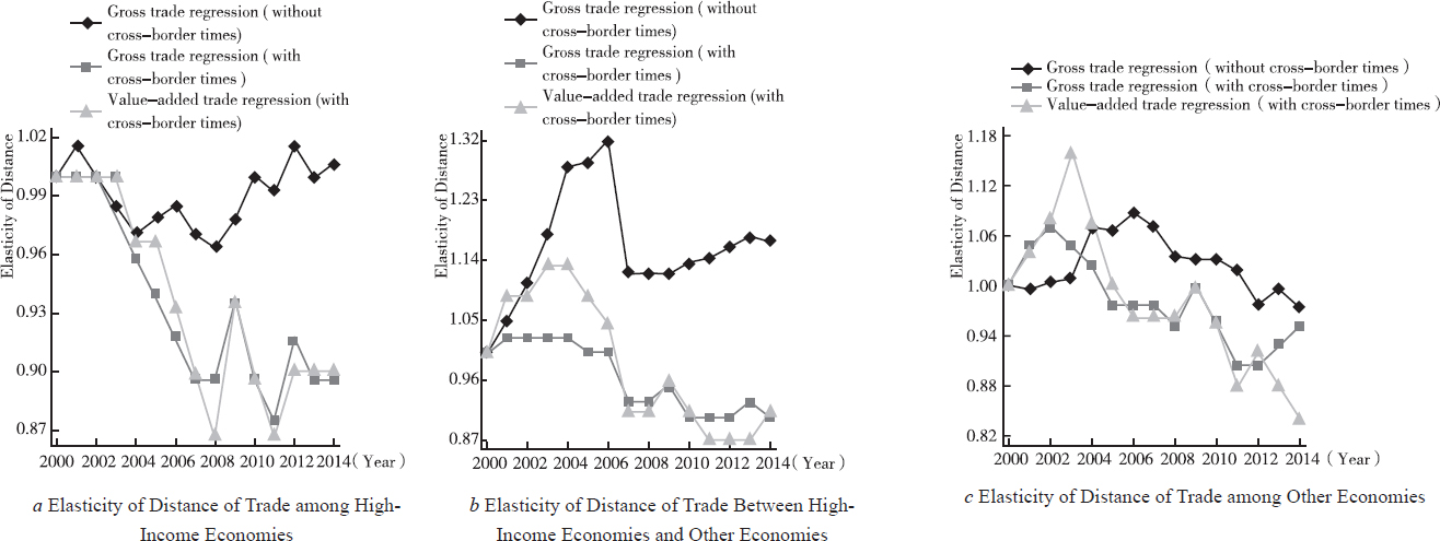
Elasticity of Distance between Economies at Different Income Levels
According to Figure 1a, the elasticity of distance showed a downward trend in 2000-2004, as seen from the regression results of gross trade among high-income economies without cross-border times, but it had increased yearly in the midst of fluctuations since 2005. This illustrates the “distance puzzle” in trade among high-income economies. With cross-border times, the elasticity of distance of gross trade regression and that of value-added trade regression for 2005-2014 was similar in the decline. This result reveals that the GVC division of labor can well explain the “distance puzzle” of trade among high-income economies.
Figure 1b depicts the changes in the elasticity of distance of trade between high-income economies and other economies, and it showed an increasing elasticity of distance in 2000-2006 and after 2007. With cross-border times, the elasticity of distance was generally diminishing, as indicated by the regression results of gross trade and value-added trade; It means that the GVC is a good explanation for the “distance puzzle” between high-income economies and other economies. [1]
Figure 1c depicts the elasticity of distance of trade among other economies. The generally diminishing elasticity of distance proved no “distance puzzle” in trade among other economies in recent years, and the decline was continued with cross-border times.
6 Conclusion
This paper explains the international trade paradox “distance puzzle” from a new perspective. Theoretically and empirically, it has proved that the GVC is an important explanation for the “distance puzzle”. Theoretically, we build a Ricardian model with multiple stages of production, by which GVC trade and traditional trade is compared in terms of the effect of distance on trade, and explains the increasing effect of GVCs on trade; The “distance puzzle” results from the growing sensitivity of trade volume to trade costs following the rapid progress of GVCs. Empirically, the Gravity Model is constructed for regression analysis of bilateral gross trade and value-added trade using cross-country panel data from the World Input-Output Database (WIOD). Without controlling the influence of the GVC, the elasticity of distance continues to increase over time to result in the “distance puzzle”. However, the “distance puzzle” disappears after cross-border times are added and the influence of the GVC is controlled. It proves that the GVC is an important explanation for the “distance puzzle”. The further robustness tests confirm the empirical results. According to heterogeneous analysis, GVCs can well explain the “distance puzzle” in intermediate goods trade, trade among high-income economies, and trade between high-income economies and low- and middle-income economies.
The conclusion has following implications. First of all, the GVC has become a dominant form of international division of labor. It has changed the picture of international trade and investment and also challenged traditional trade theories and empirical conclusions. Naturally, it should be taken into account in the theoretical and empirical studies of international trade for accurately interpreting development laws of world economy and trade. Besides, in GVC trade, trade costs such as distance hinder trade more significantly than in traditional trade; As a result, every country needs to reduce more tariffs and non-tariff trade barriers, launch efficient trade facilitating measures, cut trade costs related to time and uncertainty, and work to promote trade liberalization for world economic growth and development. Finally, this theoretical model is applicable to international trade and also to domestic inter-regional trade. As domestic value chains continue to deepen, China should make improvements to domestic transportation and communication infrastructure, the logistics service system and the modern circulation system to lower inter-regional trade costs and advance domestic market integration, through which a grand and smooth domestic economy will be shaped to speed up forming a “dual circulation” development pattern in which domestic economic cycle plays a leading role while international economic cycle remains as its extension and supplement.
Funding statement: Thanks for the support of “Integration of Implementing the Strategy of Expanding Domestic Demand and Deepening Supply-Side Structural Reform” project supported by the National Social Science Fund of China (21ZDA034), Fundamental Research Funds for the central universities, and the Central University of Finance and Economics Landmark Achievements Program. Thanks for valuable opinions from anonymous reviewers. The authors take sole responsibility for the views expressed here.
References
Antras, P., & de Gortari, A. (2020). The Geography of Global Value Chains. Econometrica, 88(4), 1553–1598.10.3386/w23456Suche in Google Scholar
Bems, R., Johnson, R. C., & Yi, K. (2011). Vertical Linkages and the Collapse of Global Trade. The American Economic Review: Papers and Proceedings, 101(3), 308–312.10.1257/aer.101.3.308Suche in Google Scholar
Bems, R., Johnson, R. C., & Yi, K. (2013). The Great Trade Collapse. Annual Review of Economics, 5(1), 375–400.10.3386/w18632Suche in Google Scholar
Bosquet, C., & Boulhol, H. (2015). What is Really Puzzling about the “Distance Puzzle”? Review of World Economics, 151(1), 1–21.10.1007/s10290-014-0201-xSuche in Google Scholar
Brun, J. F., Carrere, C., Guillaumont, P., & de Melo, J. (2005). Has Distance Died? Evidence from a Panel Gravity Model. World Bank Economic Review, 19(1), 99–120.10.1142/9789814494908_0013Suche in Google Scholar
Cairncross, F. (1997). The Death of Distance: How the Communications Revolution Will Change Our Lives. Boston: Harvard Business School Press, 1–303.Suche in Google Scholar
Caliendo, L., & Parro, F. (2015). Estimates of the Trade and Welfare Effects of NAFTA. Review of Economic Studies, 82(1), 1–44.10.3386/w18508Suche in Google Scholar
Carrère, C., & Schiff , M. (2005). On the Geography of Trade: Distance Is Alive and Well. Revue Économique, 56(6), 1249–1274.10.3917/reco.566.1249Suche in Google Scholar
Carrère, C., de Melo, J., & Wilson, J. (2013). The Distance Puzzle and Low-Income Countries: An Update. Journal of Economic Surveys, 27(4), 717–742.10.1111/j.1467-6419.2011.00715.xSuche in Google Scholar
Coe, D., Subramanian, A., & Tamirisa, N. (2007). The Missing Globalization Puzzle. IMF Staff Papers, 54(1), 34–58.10.1057/palgrave.imfsp.9450003Suche in Google Scholar
Disdier, A.C., & Head, K. (2008). The Puzzling Persistence of the Distance Effect on Bilateral Trade. The Review of Economics and Statistics, 90(1), 37–48.10.1162/rest.90.1.37Suche in Google Scholar
Dornbusch, R., Fischer, S., & Samuelson, P. (1977). Comparative Advantage, Trade, and Payments in a Ricardian Model with a Continuum of Goods. American Economic Review, 67(5), 823–39.Suche in Google Scholar
Eaton, J., & Kortum, S. (2002). Technology, Geography and Trade. Econometrica, 70(5), 1741–1779.10.1111/1468-0262.00352Suche in Google Scholar
Feenstra, R., Lipsey, R., Deng, H., Ma, A., & Mo, H. (2005). World Trade Flows: 1962-2000. NBER Working Papers, 11040.10.3386/w11040Suche in Google Scholar
Felbermayr, G., & Kohler, W. (2006). Exploring the Intensive and Extensive Margins of World Trade. Review of World Economics, 142(4), 642–674.10.1142/9789814440196_0004Suche in Google Scholar
Head, K., & Mayer, T. (2014). Gravity Equations: Workhorse, Toolkit, and Cookbook. Handbook of International Economics, 4, 131–195.10.1016/B978-0-444-54314-1.00003-3Suche in Google Scholar
Helpman, E., Melitz, M., & Rubinstein, Y. (2008). Estimating Trade Flows: Trading Partners and Trading Volumes. The Quarterly Journal of Economics, 223(2), 441–487.10.3386/w12927Suche in Google Scholar
Hong, J., & Shang, H. (2018). 40 Years of China’s Open Economy and the Prospects. Management World (Guanli Shijie), 10, 33–42.Suche in Google Scholar
Hummels, D., Ishii, J., & Yi, K. (2001). The Nature and Growth of Vertical Specialization in World Trade. Journal of International Economics, 54(1), 75–96.10.1016/S0022-1996(00)00093-3Suche in Google Scholar
Johnson, R., & Noguera, G. (2012). Accounting for Intermediates: Production Sharing and Trade in Value Added. Journal of International Economics, 86(2), 224–236.10.1016/j.jinteco.2011.10.003Suche in Google Scholar
Kee, H., & Tang, H. (2016). Domestic Value Added in Exports: Theory and Firm Evidence from China. American Economic Review, 106(6), 1402–1436.10.1596/1813-9450-7491Suche in Google Scholar
Koopman, R., Wang, Z., & Wei, S. (2014). Tracing Value-Added and Double Counting in Gross Exports. American Economic Review, 104(2), 459–494.10.3386/w18579Suche in Google Scholar
Larch, M., Norbäck, P. J., Sirries, S., & Urban, D. (2016). Heterogeneous Firms, Globalisation and the Distance Puzzle. The World Economy, 39(9), 1307–1338.10.1111/twec.12303Suche in Google Scholar
Lin, F., & Sim, N. (2012). Death of Distance and the Distance Puzzle. Economics Letters, 116(2), 225–228.10.1016/j.econlet.2012.03.004Suche in Google Scholar
Mayer, T., & Zignago, S. (2011). Notes on CEPII’s Distance Measures: The GeoDist Database. CEPII Working Paper, 2011–25.10.2139/ssrn.1994531Suche in Google Scholar
McCallum, J. (1995). National Borders Matter Canada-U.S. Regional Trade Patterns. American Economic Review, 85(3), 615–623.Suche in Google Scholar
Pan, W., & Li, G. (2018). National Value Chain and Global Value Chain in Chinese Regions: Regional Interaction and Value-Added Gains. Economic Research Journal (Jingji Yanjiu), 3, 171–186.Suche in Google Scholar
Silva, J., & Tenreyro, S. (2006). The Log of Gravity. The Review of Economics and Statistics, 88(4), 641–658.10.1162/rest.88.4.641Suche in Google Scholar
Shao, C., Li, K., & Su, D. (2018). National Value Chain and Interregional Business Cycle Synchronization: Evidence from China. Economic Research Journal (Jingji Yanjiu), 3, 187–201.Suche in Google Scholar
Timmer, M., Los, B., Stehrer, R., & de Vries, G. (2013). Fragmentation Incomes, and Jobs: An Analysis of European Competitiveness. Economic Policy, 28(76), 613–661.10.1596/1813-9450-6833Suche in Google Scholar
Wang, Z., Wei, S., Yu, X., & Zhu, K. (2017a). Measures of Participation in Global Value Chains and Global Business Cycles. NBER Working Papers, 23222.10.3386/w23222Suche in Google Scholar
Wang, Z., Wei, S., & Zhu, K. (2017b). Characterizing Global Value Chains: Production Length and Upstreamness. NBER Working Papers, 23261.10.3386/w23261Suche in Google Scholar
Yi, K. (2003). Can Vertical Specialization Explain the Growth of World Trade? Journal of Political Economy, 111(1), 52–102.10.1086/344805Suche in Google Scholar
Yi, K. (2010). Can Multistage Production Explain the Home Bias in Trade? American Economic Review, 100(1), 364–393.10.1257/aer.100.1.364Suche in Google Scholar
Yotov, Y. (2012). A Simple Solution to the Distance Puzzle in International Trade. Economics Letters, 117(3), 794–798.10.1016/j.econlet.2012.08.032Suche in Google Scholar
Zhang, J., Chen, Z., & Liu, Y. (2013). Calculation and Change Mechanism of Domestic Value Added in China’s Exports. Economic Research Journal (Jingji Yanjiu), 10, 124–137.Suche in Google Scholar
Zhang, Z., Zhu, K., & Hewings, G. (2017). The Effects of Border-Crossing Frequencies Associated with Carbon Footprints on Border Carbon Adjustments. Energy Economics, 65(1), 105–114.10.1016/j.eneco.2017.04.017Suche in Google Scholar
© 2022 Yuwan Duan, Binhan Hong, Binkai Chen, published by De Gruyter
This work is licensed under the Creative Commons Attribution 4.0 International License.
Artikel in diesem Heft
- Theoretical Logic and Empirical Facts of Consumption Structure Upgrade and Domestic Value Chain Circulation under the New Development Pattern
- Financial Shocks, Deleveraging and Macroeconomic Fluctuations in China
- Local Government Borrowing’s Expansionary Monetary Effect and Its Policy Synergy
- Distance Puzzle: An Explanation from Global Value Chain Perspective
- Exchange Rate Change, Factor Market Distortion and Company Performance
- Policy Innovation Diffusion and PPP Spatial Distribution