Voluntary Partnerships for Equally Sharing Contribution Costs: Theoretical Aspects and Experimental Evidence

Irene Maria Buso; Daniela Di Cagno; Werner Gueth; Lorenzo Spadoni

doi:10.1515/bejte-2024-0043

40% Rabatt

auf Fachbücher bei De Gruyter Brill *

Artikel

Voluntary Partnerships for Equally Sharing Contribution Costs

Theoretical Aspects and Experimental Evidence

Irene Maria Buso , Daniela Di Cagno , Werner Gueth und Lorenzo Spadoni

Veröffentlicht/Copyright: 20. Januar 2025

Veröffentlicht von

Veröffentlichen auch Sie bei De Gruyter Brill

Manuskript einreichen Informationen für Autor*innen Erkunden Sie dieses Fachgebiet

Aus der Zeitschrift The B.E. Journal of Theoretical Economics Band 25 Heft 1

Abstract

We investigate, both theoretically and experimentally, an institutional mechanism designed to enhance cooperation. In this mechanism, contributors have the option to voluntarily contribute to the public good and decide whether to join a (sub)group where partners equally share the contribution cost. Theoretically, stable cost-sharing partnerships enhance efficiency since their partners fully contribute, while outsiders would free-ride. Our data reveal that individual joining and contribution behaviors do not always align with benchmark predictions: partnerships are not always formed, and when they are, they are not always of the optimal size; partners often contribute less than maximally, and outsiders more than minimally. Nonetheless, we document systematic evidence of partnership formation and significantly improved provision of public goods across rounds.

Keywords: public good; group formation; group size; experiments

JEL Classification: C92; H41; D85

Corresponding author: Lorenzo Spadoni, Department of Economics and Law, University of Cassino and Southern Lazio, Via S. Angelo, Loc. Folcara, 03043 Cassino, Italy, E-mail: lorenzo.spadoni@unicas.it

Author contributions: The authors gratefully acknowledge the financial support of the Max-Planck-Institute for Research on Collective Goods, Kurt Schumacher Straße 10, 50113 Bonn, Germany. The authors declare that they have no known competing financial interests or personal relationships that could have appeared to influence the work reported in this paper.
Data availability: The data used to support the findings of this study are available upon request. Interested researchers may request access to the data by contacting the corresponding author: lorenzo.spadoni@unicas.it.
Use of Human Subjects: The authors confirm that all procedures were conducted in accordance with relevant laws and institutional guidelines, and that the appropriate institutional committee(s) approved them. Informed consent was obtained from all subjects participating in the experiment. Privacy rights were respected by informing participants that they would be monitored (but not recorded) using a webcam, and obtaining their acceptance of this condition.

Appendix

A Demographics

(Tables 11 and 12)

Table 11:

Descriptive statistics of demographic variables.

	Endogenous group formation
	Median	Mean	St. dev.	Min	Max
Male	0	0.38	0.48	0	1
Age	23	22.70	2.10	19	30
Economics	1	0.54	0.50	0	1
South area	1	0.55	0.49	0	1
Experience	2	2.20	0.62	1	3
Easy	1	0.76	0.42	0	1
Risk	7	6.39	2.31	0	10
	Exogenous group formation
	Median	Mean	St. dev.	Min	Max
Male	0	0.46	0.49	0	1
Age	22	22.31	2.46	18	34
Economics	1	0.61	0.48	0	1
South area	0	0.33	0.47	0	1
Experience	2	2.14	0.65	1	3
Easy	1	0.79	0.41	0	1
Risk	7	6.64	2.10	0	10
	Public good game
	Median	Mean	St. dev.	Min	Max
Male	0	0.42	0.49	0	1
Age	22	21.94	1.60	18	25
Economics	1	0.70	0.46	0	1
South area	0	0.30	0.46	0	1
Experience	2	2.14	0.58	1	3
Easy	1	0.97	0.16	0	1
Risk	6	5.58	2.00	0	10

Notes: Demographics. Male is equal to 1 = “Male”; 0 = “Female”. Age is the age in years. “Field of Study” reports the area of study: 1 = “Economics”; 2 = “Political Science”; 3 = “Law”; 4 = “Other”; in the endogenous treatment 55 % study Economics, 16 % Political Science, 23 % Law, and 6 % “Other”; in the exogenous treatment 61 % study Economics, 14 % Political Science, 21 % Law, and 4 % “Other”; in the public good treatment 70 % study Economics, 17 % Political Science, 12 % Law, and 1 % “Other”. “Economics” is a dummy variable built on “Field of Study”, and it is equal to 1 if studying “Economics”, and 0 otherwise. “Region” reports the area of origin: in the endogenous treatment 1 % are from “Abroad”, 55 % from “South”, 36 % from “Center”, and 8 % from “North”; in the exogenous treatment 4 % are from “Abroad”, 33 % from “South”, 55 % from “Center”, and 8 % from “North”; in the public good treatment 3 % are from “Abroad”, 30 % from “South”, 54 % from “Center”, and 13 % from “North”. “South Area” is a dummy variable built on “Region”, and it is equal to 1 if from “South”, and 0 otherwise. Experience is the number of experiments a subject has completed so far: 1 = “None”; 2 = “From 1 to 5”; 3 = “More than 5”. “Easy” is a dummy variable built on a “yes or no” question on the easiness of the experiment, and it is equal to 1 if easy. Risk is a self-reported measure of risk attitudes and it assumes integer values from 0 (try to avoid risk) to 10 (I like risk).

Table 12:

Balance table.

	(1)	(2)	(3)	t-test	t-test
	Endogenous	Exogenous	Public good	(1)–(2)	(1)–(3)
Male	0.38	0.46	0.42	−0.08	−0.04
Age	22.70	22.31	21.94	0.42	0.78**
Economics	0.55	0.61	0.69	−0.06	−0.14**
South area	0.55	0.33	0.30	0.21***	0.24***
Experience	2.20	2.14	2.14	0.06	0.06
Easy	0.76	0.79	0.97	0.03	−0.21***
Risk	6.39	6.64	5.58	−0.25	0.80**
Number of observations	88	72	72

Notes: Balance table. Average values are reported in columns (1), (2) and (3); mean differences are reported in the fourth column and in the fifth column. Significance of t-test: *p < 0.1, **p < 0.05, ***p < 0.01.

B Accounting for Individual Joining Behaviors

As we find many possible profiles and even the same share of ones allows for multiple profiles, we present in Table 13 only the optimal profile and the profiles with a percentage share of at least 5 % of all 88 × 12 = 1,056 profiles in each condition.

Table 13:

Joining profiles with at least 5 % of the overall choices (576).

n = 4 and α = 0.4
Joining profile 1					Joining profile 2
How many have	Your position in				How many have	Your position in
joined before you	the random sequence				joined before you	the random sequence
	4th	3rd	2nd	1st		4th	3rd	2nd	1st
0	X	1	1	1	0	X	0	0	0
1	1	1	1		1	0	0	0
2	1	1			2	0	0
3	1				3	0

Joining profile 3					Joining profile 4
How many have	Your position in				How many have	Your position in
joined before you	the random sequence				joined before you	the random sequence
	4th	3rd	2nd	1st		4th	3rd	2nd	1st
0	X	0	0	1	0	X	0	0	1
1	0	0	1		1	0	1	1
2	1	1			2	1	1
3	1				3	1

Joining profile 5					Optimal profile according to theory
How many have	Your position in				joined before you	Your position in
joined before you	the random sequence				joined before you	the random sequence
	4th	3rd	2nd	1st		4th	3rd	2nd	1st
0	X	0	1	1	0	X	0	1	0
1	0	1	1		1	0	1	0
2	1	1			2	1	0
3	1				3	0

5 different profiles emerge (in addition to the optimal one). Profile 1, “always joining”, seems to capture unconditional cooperation and can be rationalized by strong efficiency concerns. Instead Profile 2, “never joining”, could be due to not wanting to voluntarily engage in collective action, even when profitable. Profiles 3, 4, and 5 aim at the m = n grand partnership when is still possible. There is also a tendency of not joining when m = n is no longer possible (Table 14).

Table 14:

Percentage of subjects using profiles in Table 13 at least 1, 2, …, 12 rounds.

n = 4 & α = 0.4
	≥ 1	≥ 2	≥ 3	≥ 4	≥ 5	≥ 6	≥ 7	≥ 8	≥ 9	≥ 10	≥ 11	≥ 12
Profile 1	41	17	11.3	11.3	10.1	9	9	6.8	3.4	3.4	3.4	3.4
Profile 2	30	18	11.4	11.4	8	6	6	6	3.5	3.5	1	1
Profile 3	20	14	4.5	4.5	1.1	1.1	1.1	0	0	0	0	0
Profile 4	21	11	6.8	6.8	4.5	2.2	2.2	2.2	1.1	1.1	1.1	1.1
Profile 5	20	16	9	9	8	4.5	4.5	4.5	1.1	1.1	1.1	0

Table 15 summarizes the percentages of the five more frequent (and optimal) joining profiles. Altogether the five frequent profiles account for 41.10 % of the profiles in the data set. Across conditions, there are significant shares of “always joining” (11 %) and “never joining” (10 %) profiles which even increase in the last rounds (from 7 to 12) whereas optimal joining profiles are very few. Table 15 also reports the percentage of subjects adopting the same profile at least 6 times. This finding suggests inertia in the share of ones even at the individual level.

Table 15:

Frequency of joining profiles.

Type of choices	n = 4 & α = 0.4
	% choices		% subjects
	All rounds	Rounds 7-12
According to theory	2.4	2.2	1.1
Profile 1 (always join)	11	14	9
Profile 2 (never join)	10	13	6
Profile 3	5	4	1
Profile 4	5.4	3.6	2.3
Profile 5	7.3	8.5	4.5
Total	41.10	45.3	23.9

C Partnerships Formation Dynamics

(Figure 4)

Figure 4:

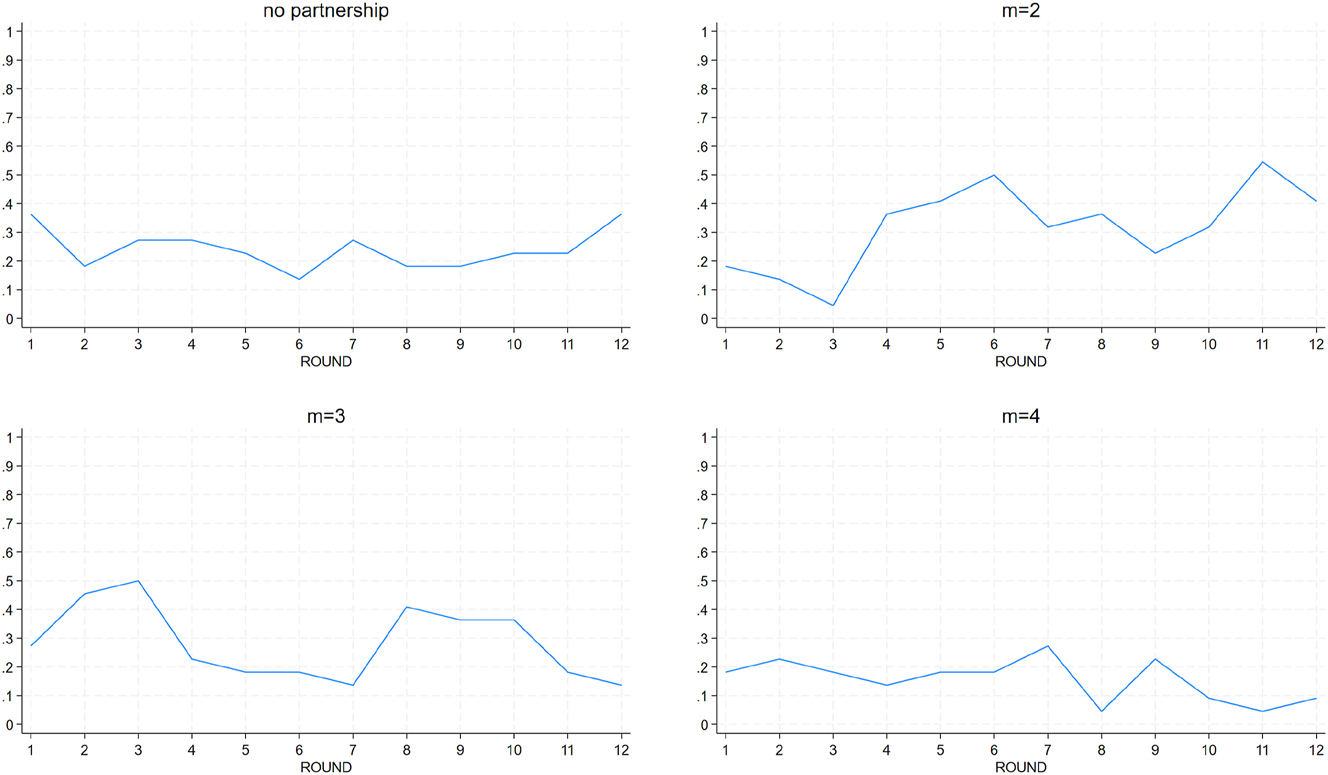
Dynamics of the frequencies of partnership sizes.

D Contribution Dynamics

(Figures 5 and 6)

Figure 5:

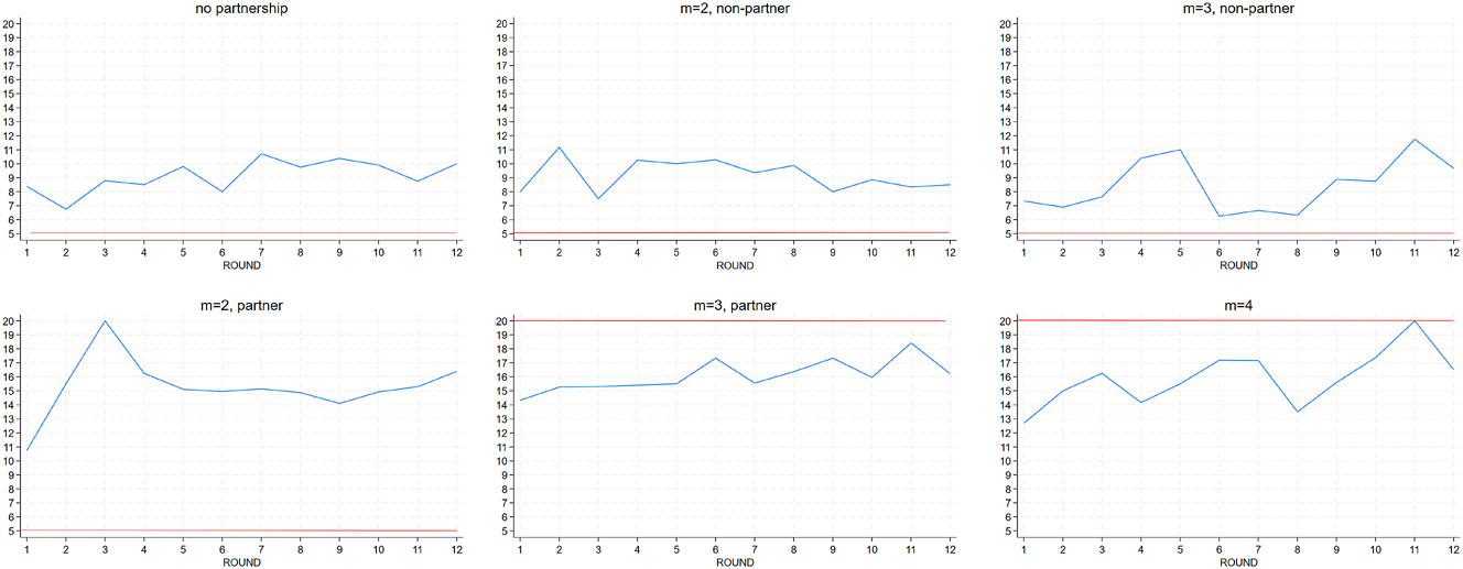
Average contribution dynamics depending on the partnership outcome in the endogenous treatment. Red lines represent the predicted values.

Figure 6:

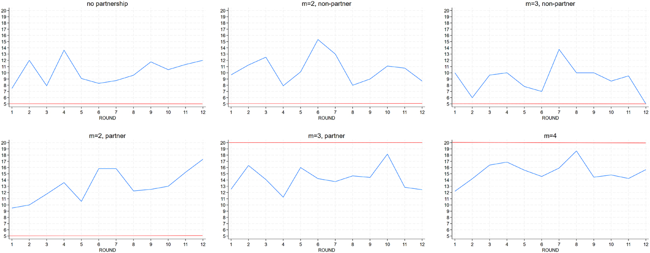
Average contribution dynamics depending on the partnership outcome in the exogenous treatment. Red lines represent the predicted values.

E Proportions of Partnership Formation

Table 16 compares the sizes of actually formed partnerships in the endogenous condition, i.e. those resulting from the actually applied random sequence, with the simulated ones, via using the respective individual joining profiles for all possible sequences. The two measures do not show differences. Simulated partnerships from 12 rounds involving 88 subjects result in 1,056 individual profile choices. These choices can be applied to 24 possible sequences, generating a total of 25,344 observations. The table also reports the proportion of partnerships in the exogenous treatment.

Table 16:

Proportion of actual partnerships formed in the endogenous and exogenous conditions, and in the simulated ones.

	Overall	m = 2	m = 3	m = 4
Endogenous	0.76	0.32	0.28	0.16
Simulated	0.76	0.32	0.28	0.16
Exogenous	0.65	0.17	0.22	0.26

F Tables with Complete Regressions

This section reports the main regression analyzes (Tables 3, 6, 8–10) making explicit the demographic controls applied (in this section, respectively, Tables 17–21). The demographic controls are gender and age of the participant, field of study, geographic region, number of past experiments, self-reported easiness of experiment and self-reported risk attitudes; these are described in detail in Appendix A.

Table 17:

Regression of the willingness to join.

Depvar: individual share of ones at round t
	(1)	(2)
Share of ones, t − 1	0.29***
	(0.03)
No partnership, t − 1 (baseline):
– Partner & m = 2, t − 1		−0.02
		(0.02)
– Non-partner & m = 2, t − 1		−0.01
		(0.02)
– Partner & m = 3, t − 1		−0.07**
		(0.03)
– Non-partner & m = 3, t − 1		−0.00
		(0.02)
– m = 4, t − 1		0.04*
		(0.02)
Final round	−0.04	−0.03
	(0.03)	(0.03)
Age	0.00	0.00
	(0.13)	(0.08)
Male	0.06	0.07
	(1.51)	(1.49)
Economic studies	−0.09*	−0.12*
	(−2.44)	(−2.42)
South Italy	0.00	0.00
	(0.02)	(0.03)
Easiness	0.00	0.00
	(0.01)	(0.00)
No previous participations (baseline):
– Between 1 and 5	−0.13*	−0.17*
	(−2.16)	(−2.20)
– More than 5	−0.10	−0.14
	(−1.58)	(−1.64)
Stated risk	0.01	0.02
	(1.57)	(1.61)
Round dummies	✓	✓
Session number	✓	✓
Observations	968	968
Number of individuals	88	88
Number of groups	11	11

The model used is a multilevel one, with two nested levels: individual and matching group. Demographic controls include gender and age of the participant, field of study, geographic region, number of past experiments, self-reported easiness of experiment. Standard errors in parentheses ***p < 0.01, **p < 0.05, *p < 0.1.

Table 18:

Regression of contribution behavior.

Depvar: contribution at round t
	(1)	(2)
Share of ones in round 1	7.10***
	(1.66)
No partnership (baseline):
– Non-partner & m = 2		0.39
		(0.44)
– Partner & m = 2		4.63***
		(0.44)
– Non-partner & m = 3		0.10
		(0.58)
– Partner & m = 3		5.79***
		(0.41)
– Partner & m = 4		5.85***
		(0.44)
Final round	1.72**	2.28***
	(0.71)	(0.63)
Age	0.02	−0.04
	(0.12)	(−0.25)
Male	0.64	0.78
	(0.85)	(1.18)
Economic studies	−2.46**	−2.20**
	(−3.17)	(−3.22)
South Italy	1.16	0.94
	(1.60)	(1.46)
Easiness	1.44	1.32
	(1.78)	(1.83)
No previous participations (baseline):
– Between 1 and 5	0.18	0.03
	(0.15)	(0.03)
– More than 5	−0.97	−1.19
	(−0.76)	(−1.07)
Stated risk	0.47**	0.49***
	(2.99)	(3.61)
Round dummies	✓	✓
Session dummies	✓	✓
Observations	1,056	968
Number of individuals	88	88

Dependent variable is the individual’s contribution in a given round of play; the model used is a multilevel one, with two nested levels: individual and matching group. Demographic controls include gender and age of the participant, field of study, geographic region, number of past experiments, self-reported easiness of experiment and self-reported risk attitudes. Standard errors in parentheses ***p < 0.01, **p < 0.05, *p < 0.1.

Table 19:

Regression of contribution behavior.

Depvar: contribution at round t
	(1)	(2)	(3)	(4)	(5)
	Overall	m = ∅	m = 2	m = 3	m = 4
Endog. formation (baseline):
– PGG standard	−2.88***
	(−2.66)
– Exog. formation	0.36	0.94	2.38	−0.49	−2.65
	(0.33)	(0.77)	(1.70)	(−0.30)	(−1.65)
Partner			4.27***	5.44***
			(7.61)	(8.39)
Exog. formation × partner			−1.87**	−0.78
			(−2.12)	(−0.86)
Final round	0.67	1.71*	2.71***	1.21	3.19
	(0.41)	(1.01)	(1.04)	(1.07)	(1.01)
Age	0.17	0.02	0.11	0.10	0.28
	(1.50)	(0.10)	(0.65)	(0.74)	(1.76)
Male	0.03	−0.56	0.03	1.27	0.85
	(0.07)	(−0.81)	(0.04)	(1.92)	(1.06)
Economic studies	−1.27**	−1.44*	−1.52*	−2.63***	−1.09
	(−2.59)	(−2.16)	(−1.98)	(−4.26)	(−1.46)
South Italy	0.13	0.37	0.31	−0.11	0.28
	(0.27)	(0.54)	(0.40)	(−0.17)	(0.36)
Easiness	0.64	0.71	0.65	0.11	0.49
	(1.01)	(0.94)	(0.77)	(0.16)	(0.57)
No previous participation (baseline):
– Between 1 and 5	−0.58	0.22	0.94	−1.33	−0.14
	(−0.81)	(0.21)	(0.83)	(−1.42)	(−0.12)
– More than 5	−1.71*	−1.02	−0.12	−2.87**	−2.60*
	(−2.14)	(−0.89)	(−0.09)	(−2.71)	(−2.17)
Stated risk	0.54***	0.52***	0.45**	0.50***	0.49**
	(5.01)	(3.52)	(2.74)	(3.55)	(2.94)
Round dummies	✓	✓	✓	✓	✓
Session dummies	✓	✓	✓	✓	✓
Observations	2,784	440	512	528	440
Number of individuals	232	157	154	156	142

Dependent variable is the individual’s contribution in a given round of play; the model used is a multilevel one, with two nested levels: individual and matching group. Demographic controls include gender and age of the participant, field of study, geographic region, number of past experiments, self-reported easiness of experiment and self-reported risk attitudes. Standard errors in parentheses ***p < 0.01, **p < 0.05, *p < 0.1.

Table 20:

Regression of contribution behavior with beliefs as regressors.

Depvar: contribution of partners at round t
	(1)	(2)	(3)	(4)	(5)	(6)
	Endogenous	Endogenous	Endogenous	Exogenous	Exogenous	Exogenous
	m = 2	m = 3	m = 4	m = 2	m = 3	m = 4
Belief on partner(s)	0.75***	0.57***	0.85***	0.76***	0.53***	0.78***
	(0.07)	(0.06)	(0.06)	(0.09)	(0.08)	(0.06)
Belief on non-partner(s)	0.06	0.07		0.14	0.15**
	(0.06)	(0.05)		(0.10)	(0.07)
Final round	2.59**	2.32**	2.10	2.06	−1.74	0.66
	(1.55)	(1.18)	(1.41)	(2.02)	(1.76)	(1.04)
Age	−0.12	−0.18	−0.01	0.21	−0.00	0.085
	(−0.56)	(−1.02)	(−0.07)	(1.07)	(−0.01)	(0.70)
Male	−0.58	1.61*	−0.69	1.01	−0.25	−0.64
	(−0.74)	(2.16)	(−1.04)	(0.76)	(−0.28)	(−0.88)
Economic studies	−0.763	−1.86*	0.14	1.74	−1.22	−0.73
	(−1.00)	(−2.54)	(0.21)	(1.42)	(−1.55)	(−1.12)
South Italy	1.85**	1.17	1.59**	−0.85	−1.00	−0.29
	(2.63)	(1.82)	(2.62)	(−0.73)	(−1.12)	(−0.43)
Easiness	1.94*	1.78*	2.13**	0.06	−2.07*	−0.66
	(2.31)	(2.36)	(3.06)	(0.04)	(−2.22)	(−0.81)
0 participations (baseline):
– Between 1 and 5	1.01	1.36	1.31	3.91*	−1.74	−0.66
	(0.94)	(1.33)	(1.37)	(2.53)	(−1.54)	(−0.74)
– More than 5	1.01	0.19	−0.07	4.17*	−2.80*	−1.455
	(0.89)	(0.17)	(−0.06)	(2.22)	(−2.08)	(−1.38)
Stated risk	−0.24	0.29	0.21	0.31	0.24	0.23
	(−1.44)	(1.84)	(1.57)	(1.06)	(1.20)	(1.54)
Round dummies	✓	✓	✓	✓	✓	✓
Session dummies	✓	✓	✓	✓	✓	✓
Observations	168	225	164	88	171	276
Number of individuals	65	76	70	51	67	72

Regressions reported in this table are multilevel ones, with two nested levels: individual and matching group. Regressions (1), (2) and (3) consider observations of partners from the endogenous condition, Regressions (4), (5) and (6) observation of partners from the exogenous condition. Belief partner(s) contribution is how much a partner believes other partner(s) to contribute; belief outsiders is how much an insider believes non-partner(s) to contribute. Demographic controls include gender and age of the participant, field of study, geographic region, number of past experiments, self-reported easiness of experiment and self-reported risk attitudes. Standard errors in parentheses ***p < 0.01, **p < 0.05, *p < 0.1.

Table 21:

Regression of non-partner contribution behavior with beliefs as regressors.

Depvar: contribution of non-partners at round t
	(1)	(2)	(3)	(4)	(5)	(6)
	Endogenous	Endogenous	Endogenous	Exogenous	Exogenous	Exogenous
	m = ∅	m = 2	m = 3	m = ∅	m = 2	m = 3
Belief on partner(s)		0.31***	−0.07		0.34***	0.35***
		(0.06)	(0.10)		(0.13)	(0.10)
Belief on non-partner(s)	0.60***	0.32***		0.65***	0.58***
	(0.07)	(0.07)		(0.07)	(0.12)
Final round	0.38	0.85	2.10	1.48	0.15	1.48
	(1.04)	(1.36)	(1.23)	(2.34)	(2.17)	(2.34)
Age	−0.07	0.19	0.22	0.12	0.28	0.12
	(0.17)	(0.25)	(0.37)	(0.17)	(0.28)	(0.17)
Male	−1.32**	−1.36	−1.57	−0.79	−1.57	−0.79
	(0.62)	(1.00)	(1.40)	(1.71)	(0.89)	(0.88)
Economic studies	−1.07	−0.80	−3.10**	−0.41	−0.71	−0.41
	(0.70)	(1.03)	(1.47)	(1.47)	(0.78)	(0.78)
South Italy	0.60	0.55	−1.28	−0.86	−0.43	−0.86
	(0.62)	(1.01)	(1.41)	(0.81)	(1.48)	(0.81)
Easiness	1.20*	−2.73***	−3.59**	0.47	2.84*	0.47
	(0.69)	(0.96)	(1.55)	(0.89)	(1.69)	(0.89)
0 participations (baseline):
– Between 1 and 5	0.42	2.10	−4.81**	−0.82	0.21	−0.82
	(1.01)	(1.47)	(2.52)	(1.19)	(1.92)	(1.19)
– More than 5	−0.99	1.30	−6.68**	−1.66	−1.91	−1.66
	(1.08)	(1.69)	(2.93)	(1.42)	(2.33)	(1.42)
Stated risk	0.27**	0.36*	0.52**	0.42**	−0.02	0.42
	(0.13)	(0.18)	(0.19)	(0.29)	(0.33)	(0.19)
Round dummies	✓	✓	✓	✓	✓	✓
Session dummies	✓	✓	✓	✓	✓	✓
Observations	256	168	75	184	88	57
Number of individuals	87	62	38	70	53	39

Regressions reported in this table are multilevel ones, with two nested levels: individual and matching group. Regressions (1), (2) and (3) consider observations of non partners and when there is no partership from the endogenous treatment, Regressions (4), (5) and (6) observation of non-partners and when there is no partership from the exogenous treatment. Belief partner(s) contribution is how much a non-partner believes partner(s) to contribute; belief outsiders is how much an outsider believes other non-partner(s) to contribute – if there is no partnership non-partner beliefs indicated beliefs on other group members. Demographic controls are described in the Appendix and include gender and age of the participant, economics, south area, experience, self-reported easiness of experiment and self-reported risk attitudes. Standard errors in parentheses ***p < 0.01, **p < 0.05, *p < 0.1.

The main tendency that emerges is that students in economics and subjects more experienced with experiments are less willing to join and tend to contribute less. Also, the propensity to take risk is positively related to contribution.

G Instructions (Translated Version)

G.1 EnPGG

G.1.1 Instructions General Description of the Experiment

Welcome to this experiment!

In this experiment, completely computerized, you and the other participants will make choices. Your choices and those of the other participants will determine your earnings for the experiment according the rules that will be explained in these instructions.

In addition to the earnings for the experiment, you will receive 6 euros for showing up and answering a short questionnaire at the end of the experiment.

The experiment consists of 12 rounds.

You have the opportunity to earn points (ECU) in each round that will be converted into Euro at an exchange rate of 1 point = €0.5.

At the end of the experiment, one round is randomly selected for payment. The payment will be implemented using Prolific. The data of the experiment (your choices) are anonymous: the experimenter will not be able to connect your name to your choices.

At the beginning of the experiment, you will be randomly matched by the computer with other 3 participants. You and the other selected participants will form a group of 4 in each round.

Note that after each round the composition of the group will change such that you will always interact with a group different from the group of the previous round for at least one participant. Note that you will not learn who the other members of your group are, neither during nor after today’s session.

In each round you will make two types of choices. First, you will decide to join or not an “Initiative” related to a “Project” common to all the group members; the second choice will concern how much to contribute to the “Project”.

After these choices, in each round you will be asked to answer few questions whose answers will not have any relevance for your earnings.

After each round you will learn the number of points (ECU) earned in that round. At the end of the experiment it will be shown on the screen which round has been drawn for payment and you will be recalled about the points earned in that round which will be your earnings for the experiment. Before the payment, you will be asked to answer few questions not relevant for the payment and that will preserve your anonymity. It is very important that you completely understand the instructions and the way your earnings are related to your decisions. In order to check your understanding, at the beginning of the experiment we will ask you to answer some questions about payoff calculation. If at any point during the experiment you have a question, please contact the experimenters using the chat or the microphone, and you will be answered privately.

G.1.2 The Decision to Join the “Initiative” Related to the “Project”

In each round you and the other group members will choose sequentially whether to join or not the “Initiative”.

Note that the position in the sequence for you and the other group members will be chosen randomly by the computer.

Before you are let aware of your actual position in the sequence (i.e. if you are the first, the second, the third or the fourth, you will be asked whether you want to join or not the “Initiative” for every possible position in this sequence and for every possible number of participants that have already joined the group before you).

Once you have chosen whether to join or not in every possible scenario, the actual position in the sequence for each of you will be randomly drawn, and choices in the corresponding scenario will be implemented.

The computer will inform you about the existence of the “Initiative” in your group, how many group members are part of it, and if you are in.

Remember that participating to the “Initiative” is voluntary. Hence, it may happen that less than two members of your group choose to join; in this case, the “Initiative” will not exist.

G.1.3 The Decision of How Much to Contribute to the “Project”

Each of you will be endowed with 25 points at the beginning of each round. You will choose simultaneously and independently whether and how much to contribute to a “Project” with your endowment: each of you have to choose an integer amount between and including 5 and 20 to devote to the “Project”.

Your earnings from the “Project” in each round will be calculated as follows:

If you chose to join the “Initiative” and this exists, your earnings are equal to:

Your Endowment – [(your contribution + the contribution of the other member(s) of the “Initiative”)/the member of the “Initiative” including you] + α (your contribution + the contribution of the other group members).

Note that in this case your actual contribution may be different from the amount you stated and it will be equal to the average contribution of the members of the “Initiative”.
If you chose to not join the “Initiative” or if this does not exist, your earnings are equal to:

Your Endowment – your contribution + α (your contribution + the contribution of the other group members).

In every round the value of alpha will be equal to 0.4.

G.2 StPGG

G.2.1 Instructions General Description of the Experiment

Welcome to this experiment!

In this completely computerized experiment, you and the other participants will make some choices. Your choices and those of the other participants will determine your earnings for the experiment according to the rules explained in these instructions.

In addition to the earnings for the experiment, you will receive 6 euros for showing up and answering a short questionnaire at the end of the experiment.

The experiment consists of 12 rounds.

In each round, you will have the opportunity to earn points (ECU) that will be converted into EURO at the end of the experiment at an exchange rate of 1 ECU = 0.5 EURO.

At the end of the experiment, one round will be randomly selected for payment. The payment will be implemented using PayPal. The data from the experiment (your choices) are completely anonymous: the experimenters will not be able to connect your name to your choices.

At the beginning of the experiment, you will be randomly matched with 3 other participants from your session. You and the other selected participants will form a group of 4 in each round.

Note that after each round, the composition of the group will change such that you will always interact with a group different from the group of the previous round for at least one participant. Also note that you will not learn who the other members of your group are, neither during nor after today’s session.

In each round of the experiment, you will make a decision related to a “Project” common to all group members.

After these choices, in each round, you will be asked to answer a few questions whose answers will not affect your earnings.

After each round, you will learn the number of points (ECU) earned in that round. At the end of the experiment, it will be shown on the screen which round has been drawn for payment, and you will be reminded of the points earned in that round, which will be your earnings for the experiment. Before the payment, you will be asked to fill out a brief questionnaire, which is anonymous and not incentivized.

It is very important that you read the instructions carefully to understand how your earnings are related to your decisions. To check your understanding, at the beginning of the experiment, we will ask you to answer some questions about payoff calculation.

If you have any questions during the experiment, please contact the experimenters using the chat or the microphone, and you will be answered privately.

G.2.2 The Decision on How Much to Contribute to the “Project”

At the beginning of each round, each of you will be endowed with 25 points (ECU). You will choose, independently and simultaneously from the other participants, whether and how much you want to contribute to a “Project” with your endowment. Note: You must choose to contribute to the “Project” an integer amount between and including 5 and 20 points (ECU).

Your earnings from the “Project” in each round will be calculated as follows:

Your Endowment – [your contribution + α * (your contribution + the contribution of the other members of your group)].

In every round, the value of α will be 0.4.

Enjoy!

G.3 ExPGG

G.3.1 Instructions General Description of the Experiment

Welcome to this experiment!

In addition to the earnings from the experiment, you will receive 6 euros for showing up and answering a short questionnaire at the end of the experiment.

The experiment consists of 12 rounds.

You have the opportunity in each round to gain points (ECU) that will be converted into EURO at the end of the experiment at an exchange rate of 1 ECU = 0.5 EURO.

At the end of the experiment, one round is randomly selected for payment. The payment will be implemented via PayPal. The data from the experiment (your choices) are anonymous: the experimenters will not be able to connect your name to your choices.

At the beginning of the experiment, you will be randomly matched by the computer with 3 other participants in your session. You and the other selected participants will form a group of 4 in each round.

Note that after each round, the composition of your group will change such that you will always interact with a group different for at least one participant from the group of the previous round. Also note that you will not learn who the other members of your group are, neither during nor after today’s session.

In each round of the experiment, you must make a decision related to a “Project” common to all the group members.

After these choices, in each round, you will be asked to answer a few questions whose answers will not have any relevance for your earnings.

After each round, you will learn the number of points (ECU) earned in that round. At the end of the experiment, it will be shown on your screen which round has been drawn for payment, and you will be reminded of the points earned in that round, which will be your earnings for the experiment. Before the payment, you will be asked to fill out a brief questionnaire, which is anonymous and not incentivized.

It is important that you read the instructions carefully to properly understand how your earnings are related to your and the other participants’ decisions. To check your understanding, at the beginning of the experiment, we will ask you some questions about payoff calculation.

If you have any doubts, please contact the experimenters using the chat or the microphone, and you will be answered privately.

G.3.2 The Decision to Join the “Initiative” Related to the “Project”

At the beginning of each round, before you and the other members of your group make your choice about the common “Project,” the computer will randomly select whether each member of the group (including yourself) will join the “Initiative” connected to the common “Project.” Based on this random draw, if at least 2 out of the 4 members of your group join the “Initiative,” it will exist; otherwise, if none or only one of the group members join the “Initiative,” it will not exist.

If the “Initiative” exists, it could be formed by 2, 3, or 4 (all) members of the group. Note that if only 2 members join, the other 2 will not be part of it; if 3 members join, the remaining member will not be part of it.

Before you make your decision about the common “Project,” the computer will inform you whether the “Initiative” exists or not among your group participants, how many of them are part of it, and whether you are in.

G.3.3 The Decision of How Much to Contribute to the “Project”

At the beginning of each round, each participant will be endowed with 25 ECU. You must decide, independently and simultaneously from the other participants, whether and how much you want to contribute to the common “Project” with your endowment. Note: You must choose an integer amount between and including 5 and 20 to devote to the “Project.”

Your earnings from the “Project” in each round will be calculated as follows:

If the “Initiative” exists and you are in, your earnings are given by: Your Endowment – [your contribution + the other member(s) participating in the “Initiative” contribution/the members of the “Initiative” including you] + α * (your contribution + the contribution of the other group members).

Note that in this case, your actual contribution may be different from the amount you stated, and will be equal to the average contribution that the members of the “Initiative” independently decide to contribute to the “Project.”
If the “Initiative” does not exist, or if it exists but you are not in, your earnings are calculated as follows: Your Endowment – your contribution + α * (your contribution + the contribution of the other group members).

In every round, the value of α will be 0.4.

Enjoy!

References

Andreoni, J., and L. K. Gee. 2012. “Gun for Hire: Delegated Enforcement and Peer Punishment in Public Goods Provision.” Journal of Public Economics 96 (11–12): 1036–46. https://doi.org/10.1016/j.jpubeco.2012.08.003.Suche in Google Scholar

Barrett, S. 2003. Environment and Statecraft: The Strategy of Environmental Treaty-Making: The Strategy of Environmental Treaty-Making. Oxford: OUP Oxford.10.1108/meq.2003.14.5.622.3Suche in Google Scholar

Booth, A. L. 1985. “The Free Rider Problem and a Social Custom Model of Trade Union Membership.” Quarterly Journal of Economics 100 (1): 253–61. https://doi.org/10.2307/1885744.Suche in Google Scholar

Burger, N. E., and C. D. Kolstad. 2009. “Voluntary Public Goods Provision, Coalition Formation, and Uncertainty.” Technical Report. National Bureau of Economic Research.10.3386/w15543Suche in Google Scholar

Buso, I. M., D. Di Cagno, L. Ferrari, V. Larocca, L. Lorè, F. Marazzi, L. Panaccione, and L. Spadoni. 2021. “Lab-like Findings from Online Experiments.” Journal of the Economic Science Association 7 (2): 184–93. https://doi.org/10.1007/s40881-021-00114-8.Suche in Google Scholar

Chen, Y., and S. X. Li. 2009. “Group Identity and Social Preferences.” The American Economic Review 99 (1): 431–57. https://doi.org/10.1257/aer.99.1.431.Suche in Google Scholar

Chen, D. L., M. Schonger, and C. Wickens. 2016. “Otree—An Open-Source Platform for Laboratory, Online, and Field Experiments.” Journal of Behavioral and Experimental Finance 9: 88–97. https://doi.org/10.1016/j.jbef.2015.12.001.Suche in Google Scholar

Dannenberg, A., and C. Gallier. 2020. “The Choice of Institutions to Solve Cooperation Problems: A Survey of Experimental Research.” Experimental Economics 23 (3): 716–49. https://doi.org/10.1007/s10683-019-09629-8.Suche in Google Scholar

Dannenberg, A., A. Lange, and B. Sturm. 2014. “Participation and Commitment in Voluntary Coalitions to Provide Public Goods.” Economica 81 (322): 257–75. https://doi.org/10.1111/ecca.12073.Suche in Google Scholar

Dillbary, J. S., C. Metcalf, and B. Stoddard. 2021. “Incentivized Torts: An Empirical Analysis.” Northwestern University Law Review 115: 1337.Suche in Google Scholar

Gallier, C., M. Kesternich, and B. Sturm. 2017. “Voting for Burden Sharing Rules in Public Goods Games.” Environmental and Resource Economics 67: 535–57. https://doi.org/10.1007/s10640-016-0022-6.Suche in Google Scholar

Gerber, A., J. Neitzel, and P. C. Wichardt. 2013. “Minimum Participation Rules for the Provision of Public Goods.” European Economic Review 64: 209–22. https://doi.org/10.1016/j.euroecorev.2013.09.002.Suche in Google Scholar

Greiner, B. 2015. “Subject Pool Recruitment Procedures: Organizing Experiments with Orsee.” Journal of the Economic Science Association 1 (1): 114–25. https://doi.org/10.1007/s40881-015-0004-4.Suche in Google Scholar

Gürdal, M. Y., Ö. Gürerk, and M. Yahşi. 2021. “Culture and Prevalence of Sanctioning Institutions.” Journal of Behavioral and Experimental Economics 92: 101692. https://doi.org/10.1016/j.socec.2021.101692.Suche in Google Scholar

Gürerk, Ö. 2013. “Social Learning Increases the Acceptance and the Efficiency of Punishment Institutions in Social Dilemmas.” Journal of Economic Psychology 34: 229–39. https://doi.org/10.1016/j.joep.2012.10.004.Suche in Google Scholar

Gurerk, O., B. Irlenbusch, and B. Rockenbach. 2006. “The Competitive Advantage of Sanctioning Institutions.” Science 312 (5770): 108–11. https://doi.org/10.1126/science.1123633.Suche in Google Scholar

Gürerk, Ö., B. Irlenbusch, and B. Rockenbach. 2014. “On Cooperation in Open Communities.” Journal of Public Economics 120: 220–30. https://doi.org/10.1016/j.jpubeco.2014.10.001.Suche in Google Scholar

Kesternich, M., A. Lange, and B. Sturm. 2014. “The Impact of Burden Sharing Rules on the Voluntary Provision of Public Goods.” Journal of Economic Behavior & Organization 105: 107–23. https://doi.org/10.1016/j.jebo.2014.04.024.Suche in Google Scholar

Kocher, M. G., P. Martinsson, E. Persson, and X. Wang. 2016. “Is There a Hidden Cost of Imposing a Minimum Contribution Level for Public Good Contributions?” Journal of Economic Psychology 56: 74–84. https://doi.org/10.1016/j.joep.2016.05.007.Suche in Google Scholar

Kosfeld, M., A. Okada, and A. Riedl. 2009. “Institution Formation in Public Goods Games.” The American Economic Review 99 (4): 1335–55. https://doi.org/10.1257/aer.99.4.1335.Suche in Google Scholar

Kurzban, R., K. McCabe, V. L. Smith, and B. J. Wilson. 2001. “Incremental Commitment and Reciprocity in a Real-Time Public Goods Game.” Personality and Social Psychology Bulletin 27 (12): 1662–73. https://doi.org/10.1177/01461672012712009.Suche in Google Scholar

McEvoy, D. M. 2010. “Not It: Opting Out of Voluntary Coalitions that Provide a Public Good.” Public Choice 142: 9–23. https://doi.org/10.1007/s11127-009-9468-1.Suche in Google Scholar

McEvoy, D. M., T. L. Cherry, and J. K. Stranlund. 2015. “Endogenous Minimum Participation in International Environmental Agreements: An Experimental Analysis.” Environmental and Resource Economics 62: 729–44. https://doi.org/10.1007/s10640-014-9800-1.Suche in Google Scholar

McEvoy, D. M., J. J. Murphy, J. M. Spraggon, and J. K. Stranlund. 2010. “The Problem of Maintaining Compliance within Stable Coalitions: Experimental Evidence.” Oxford Economic Papers 63 (3): 475–98. https://doi.org/10.1093/oep/gpq023.Suche in Google Scholar

Morgenstern, R. D., W. A. Pizer, and W. A. Pizer. 2007. Reality Check: The Nature and Performance of Voluntary Environmental Programs in the United States, Europe, and Japan. Washington DC: Resources for the Future.Suche in Google Scholar

Naylor, R., and M. Cripps. 1993. “An Economic Theory of the Open Shop Trade Union.” European Economic Review 37 (8): 1599–620. https://doi.org/10.1016/0014-2921(93)90123-r.Suche in Google Scholar

Nicklisch, A., K. Grechenig, and C. Thöni. 2016. “Information-sensitive Leviathans.” Journal of Public Economics 144: 1–13. https://doi.org/10.1016/j.jpubeco.2016.09.008.Suche in Google Scholar

Oliver, P. 1980. “Rewards and Punishments as Selective Incentives for Collective Action: Theoretical Investigations.” American Journal of Sociology 85 (6): 1356–75. https://doi.org/10.1086/227168.Suche in Google Scholar

Orzen, H. 2008. “Fundraising through Competition: Evidence from the Lab.” Technical Report. CeDEx Discussion Paper Series.Suche in Google Scholar

Palan, S., and C. Schitter. 2018. “Prolific. Ac—A Subject Pool for Online Experiments.” Journal of Behavioral and Experimental Finance 17: 22–7. https://doi.org/10.1016/j.jbef.2017.12.004.Suche in Google Scholar

Selten, R. 1975. “Reexamination of the Perfectness Concept for Equilibrium in Bargaining Model.” Econometrica 52 (1): 352–1.10.1007/BF01766400Suche in Google Scholar

Selten, R., and W. Güth. 1982. Equilibrium Point Selection in a Class of Market Entry Games, Games, Economic Dynamics, and Time Series Analysis, 101–16. Heidelberg: Physica-Verlag HD.10.1007/978-3-662-41533-7_6Suche in Google Scholar

Sutter, M., and H. Weck-Hannemann. 2003. “On the Effects of Asymmetric and Endogenous Taxation in Experimental Public Goods Games.” Economics Letters 79 (1): 59–67. https://doi.org/10.1016/s0165-1765(02)00288-4.Suche in Google Scholar

Sutter, M., S. Haigner, and M. G. Kocher. 2010. “Choosing the Carrot or the Stick? Endogenous Institutional Choice in Social Dilemma Situations.” The Review of Economic Studies 77 (4): 1540–66. https://doi.org/10.1111/j.1467-937x.2010.00608.x.Suche in Google Scholar

Tyran, J.-R., and L. P. Feld. 2006. “Achieving Compliance when Legal Sanctions Are Non-deterrent.” The Scandinavian Journal of Economics 108 (1): 135–56. https://doi.org/10.1111/j.1467-9442.2006.00444.x.Suche in Google Scholar

Zelmer, J. 2003. “Linear Public Goods Experiments: A Meta-Analysis.” Experimental Economics 6 (3): 299–310. https://doi.org/10.1023/a:1026277420119 10.1023/A:1026277420119Suche in Google Scholar

Received: 2024-03-18

Accepted: 2025-01-07

Published Online: 2025-01-20

Sie haben derzeit keinen Zugang zu diesem Inhalt.

Artikel in diesem Heft

https://doi.org/10.1515/bejte-2024-0043

Schlagwörter für diesen Artikel

public good; group formation; group size; experiments