A molecular mechanics implementation of the cyclic cluster model
-
Juan Diego Samaniego-Rojas
 ,
Robin Gaumard
,
Robin Gaumard

Abstract
The implementation of the cyclic cluster model (CCM) for molecular mechanics is presented in the framework of the computational chemistry program deMon2k. Because the CCM is particularly well-suited for the description of periodic systems with defects, it can be used for periodic QM/MM approaches where the non-periodic QM part is treated as a defect in a periodic MM surrounding. To this end, we present here the explicit formulae for the evaluation of the Ewald sum and its first- and second-order derivatives as implemented in deMon2k. The outlined implementation was tested in molecular dynamics (MD) simulations and periodic structure optimization calculations. MD simulations of an argon system were carried out using the Nosé-Hoover chain (NHC) thermostat and the Martyna-Tobias-Klein (MTK) barostat to control the temperature and pressure of the system, respectively. For the validation of CCM structure optimization a set of molecular crystals were optimized using the Ewald method for the evaluation of the electrostatic interactions. Two optimization procedures for the determination of the atomic positions and CCM cell parameters were tested. Our results show that the simultaneous optimization of the atomic positions and cell parameters is most efficient.
1 Introduction
With the rise of hybrid quantum mechanical/molecular mechanical (QM/MM) schemes [1], [2] new atomistic approaches for the simulation of condensed matter systems have become available. In comparison to pure MM simulations, QM/MM calculations permit the incorporation of chemical bond breaking and forming in the QM region. Therefore, they are very well suited for the study of chemical reactions in solutions, on surfaces or in the bulk. For all these applications it is beneficial to have QM regions as large as possible. Thus, the QM method for such QM/MM applications must not only be accurate and reliable but also computationally efficient. A possible choice in this respect is auxiliary density functional theory (ADFT) [3], [4] as implemented in deMon2k [5]. This is one of the main motivations behind the QM/MM implementation efforts in deMon2k over the last decade [6], [7]. For a comprehensive overview we refer the interested reader to [8].
Although polarizable force fields are implemented in some versions of deMon2k [7], we restrict ourselves for the here described development to non-polarizable force fields. With this setup for the QM/MM methodology, we now need appropriate models for the simulations. The droplet model, Figure 1 (left), consisting of a QM and an MM region embedded into a polarizable continuum has gained much popularity in deMon2k QM/MM calculations. It is well suited for the simulation of solutions where QM molecules, free or solvated, are embedded in MM solvents [7], [9]. However, it is not suitable for the description of solids or for NPT molecular dynamics (MD) simulations.

Droplet (left) and CCM (right) models for QM/MM solution systems. A ball-and-stick representation is used for the QM molecules and a stick-only representation for MM molecules.
To overcome this limitation we are developing at Cinvestav the QM/MM cyclic cluster model (CCM) as depicted in Figure 1 (right). In this model, the QM region, represented by the ball-and-stick molecules in Figure 1, is a QM defect in a periodic MM-CCM system. The CCM is an appropriate model for systems where the periodicity has been lifted by local defects because it avoids direct interactions between them [10]. The computational structure of the CCM we use in this work for MM systems is closely related to the quasimolecular large unit cell model of Dobrotvorskii and Evarestov [11]. A detailed comparison of the two models is given in the literature [12], [13]. Although the CCM has been implemented at the semiempirical [14], [15], [16], [17], ab initio [18], and density-functional [19], [20] levels of theory, we are not aware of any implementation in the MM framework. Therefore, we present here such an implementation in deMon2k as the first step towards a QM/MM-CCM methodology.
This work is organized as follows. In Section 2, we present the theory and implementation details of the CCM scheme for the calculation of the energy and energy derivatives within the MM branch of the deMon2k program. In the next section, we describe our Ewald sum implementation for the efficient evaluation of long-range Coulomb interactions. This is an essential part for the appropriate description of polar systems, and it represents the energy component that requires most attention for its use in structure optimization methods and MD simulations. Thus, we present explicit formulae for the evaluation of analytic first- and second-order derivatives of these sums. The computational methodology is presented in Section 4. Finally, in Section 5, the here developed MM-CCM methodology is validated for molecular dynamics and optimization applications. To this end, MD simulations in the isobaric-isothermal (NPT) ensemble of liquid argon and structure optimizations of molecular crystals with MM-CCM are presented and discussed. Final conclusions are given in the last section of the article.
2 MM-CCM implementation
2.1 Molecular mechanics
The MM energy terms can be classified in two categories depending on whether the interacting atoms are bonded or not. Therefore, the information about the molecular connectivity is required. In deMon2k, this is either given by the user in the input, or automatically generated from the distances between the MM atoms. The resulting MM energy is given by:
The first four terms represent the bond stretching, angle bending, torsion and out-of-plane (or improper) torsion energies. The first two terms in eq. (1) are harmonic potentials. The following two are periodic functions. For the van der Waals and the point charge Coulomb energy terms, the well-known 12-6 Lennard-Jones and Coulomb potentials are used:
Throughout this work, capital latin letters, A, B, … denote atoms. The corresponding bold letters are the atomic position vectors.
As for the van der Waals interactions between MM atoms, the coupling of the QM and MM subsystems in the additive QM/MM scheme implemented in deMon2k is also modelled by eq. (2). In that case, the A and B indices represent QM and MM atoms, respectively. For the calculation of the QM/MM ϵ AB and σ AB combination rules of atomic parameters, i.e. ϵ A (QM atom) and ϵ B (MM atom) as well as σ A (QM atom) and σ B (MM atom), are used [8]. Therefore, in QM/MM calculations such force field parameters are required for MM and QM atoms. In this work, these atomic parameters are taken from the OPLS force field [21], [22], whereas diatomic parameters are obtained through combination rules which are given by a geometric average by default. Thus, the epsilon parameter for the interaction between two atoms is given by:
A similar formula is used for the σ AB parameter.
Molecular dynamics and local optimization procedures for the time propagation and structure relaxation of molecular systems, respectively, require first- and second-order analytic derivatives of all terms in eq. (1). Explicit formulae for the implementation of this energy and its derivatives in deMon2k can be found in [8]. They can be used alone or in combination with QM gradients and second-derivatives for structure optimizations, MD simulations or molecular property calculations. Simulations in the canonical (NVT) ensemble are carried out using the extended system approach with the Nosé-Hoover chain (NHC) thermostat [23], [24]. More recently, the pressure-controlling algorithm from Martyna, Tobias and Klein (MTK) [25] has been implemented in deMon2k, allowing simulations in the NPT ensemble, too. The necessary volume definition for the barostat is provided by the CCM cluster.
2.2 The cyclic cluster model
In deMon2k, periodicity is introduced in the form of the cyclic cluster model (CCM) in which cyclic boundary conditions are directly applied to a cluster. Thus, the system remains finite. The CCM cluster must be a portion of a system that can be used to generate its periodicity. In principle, a primitive unit cell (PUC) can be used as CCM cluster, but for physically meaningful results a large unit cell (LUC) or supercell is usually considered. Therefore, electronic structure methods developed for molecular quantum chemistry, i.e. for finite systems, can be used in CCM calculations. The same applies to MM methods.
For the case of systems with defects, as mentioned above, direct defect-defect interactions are excluded in the CCM by construction. Consider Figure 2, where a two-dimensional system with four atoms is shown. The central cell, with solid black lines standing for the cell vectors a x and a y , represents the cluster with real atoms denoted by red dots. The replicas around the central cell contain translations of these atoms, known as virtual atoms in CCM, depicted by blue dots. As is shown in the figure, the interactions for atom A in the cluster are limited to a region (shown in light green) formed by the restriction that the projection of the distance vector between two atoms onto an edge of the cell is not allowed to exceed half the length of that edge. Three cases are possible for the surrounding atoms: (i) they are inside the interaction region; (ii) they are on its edge; or (iii) they are outside the interaction region. These are the cases of the B, C and D atoms in Figure 2, respectively. No modification of the interatomic vector is required in the first case. However, for the second and third cases, these vectors need to be translated by the same translation vector as that of the cell containing the interacting virtual atom. In addition, for the particular case of the AC interaction, we observe that the real atom in cell 0 and the virtual atom in cell 5 (indicated by the superscript in the interatomic distance vectors in the figure) both fullfill the interaction restriction. In order to avoid double counting of interactions, it is possible to neglect one of them. However, this will cause a dipole moment in ionic systems and lead to unphysical results. To overcome this problem, we consider all the interactions and then take an average as suggested in [15]. By imposing these restrictions, the interaction region around each atom takes the shape of a Wigner-Seitz cell (WSC) generated from the (large) unit cell. As a result, an atom cannot interact with one of its translationally equivalent atoms and, therefore, direct defect-defect interactions are avoided.
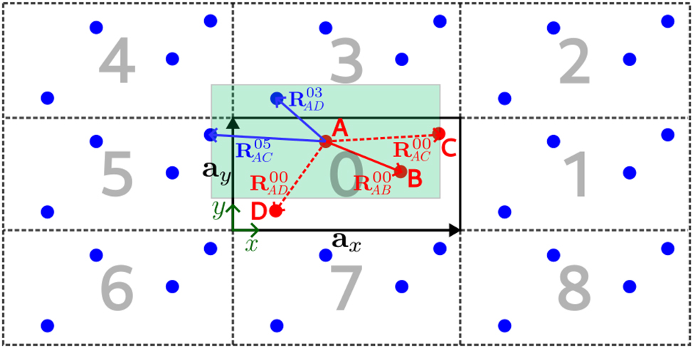
Two-dimensional CCM cluster (zero cell) with cell vectors a x and a y containing four atoms (red dots). The CCM cluster replicas 1 to 8 with virtual atoms (blue dots) are indicated by dashed lines. The light green area marks the interaction region for atom A. Interatomic distance vectors are denoted by the letter R with a subindex indicating the start and end atoms and a superindex indicating the cell to which these atoms belong. Dashed interaction vectors are used to indicate that these vectors need to be modified. See text for details.
Eq. (1) can be directly used in CCM by simply modifying the interatomic distance vectors. For the case of ionic systems, where long-range Coulomb interactions need to be calculated, the expression in eq. (3) will be replaced by the corresponding Ewald sum, as discussed in Section 3, for its efficient calculation. Besides this change, the expressions for the energy, gradients and second-order energy derivatives of eq. (1) can be directly used for MM-CCM systems. Only the derivatives with respect to the cell parameters need to be added as outlined in the following subsection.
2.3 Energy derivatives
In the following, we assume that each edge of the cell lies along one of the Cartesian coordinate axes. Therefore, the corresponding cell vectors in our setup have only one non-vanishing component. For this reason, they will be addressed using only one index. Furthermore, from here on we will use the term cell parameter to refer to the cell vectors only component. Note that these cell parameters are also the lengths of the cell. For the calculation of CCM energy derivatives, we first define the relationship between the atomic position vectors and the cell parameters of the CCM cluster. This can be expressed as follows:
In eq. (5), f Aλ (λ = x, y, z) represent the components of the atomic position vector A in the basis of the cell vectors a x , a y and a z , also known as fractional coordinates. Therefore, the derivative of the atomic position vector with respect to a cell parameter is given by the corresponding fractional coordinate. In our setup, the fractional coordinates are simply the ratio f Aλ = A λ /a λ , where a λ is the magnitude of a λ and A λ the corresponding component of the atomic position vector. From this expression, one can obtain the derivative with respect to an atomic coordinate in terms of a cell parameter and vice versa. Therefore, we can expand energy derivatives with respect to a cell parameter by the calculated atomic gradient component and the corresponding fractional coordinate:
In our derivatives formulae Greek letters λ, η, … denote the Cartesian coordinates x, y and z. Second-order derivatives can be immediately obtained from the previous equation by recognizing the first-order differential operator with respect to the cell parameter a λ in it and building the second-order as:
Finally, it is also possible to obtain mixed second-order derivatives where the differentiation is with respect to one atomic coordinate and one cell parameter. For this purpose, we can start from eq. (6) and derive it with respect to an atomic coordinate. This yields:
Equations (6)–(8) can be applied to all terms in eq. (1) as long as their dependency on the cell parameters is only through the atomic positions. We will see in the next section that this is not the case for the Ewald part of the energy.
3 The Ewald summation method
In order to extend the CCM to polar systems, long-range Coulomb interactions must be added [16]. Unfortunately, eq. (3) is only conditionally convergent when applied to periodic (infinite) systems. Therefore, the summation order must be defined first. A possibility is adding replicas in a spherical way according to their distances to the central unit cell. This definition makes it possible to transform the original sum in eq. (3) into two rapidly and totally convergent sums using the method of Ewald [26], [27], [28], [29], [30], [31], [32]. This changes the MM energy expression to:
The main idea of this approach is to place a charge distribution at the location of every point charge q A , but with opposite sign, see Figure 3, left.

One dimensional system with the charge density distributions used in the Ewald method. Point charges and shielding charge distributions (left) give rise to the direct part of the potential, while the compensating charge distributions (right) generate the part of the potential evaluated in reciprocal space.
The potential arising from the point charges and the charge distributions can be rapidly calculated in direct space. A second set of compensating charge distributions needs to be added to recuperate the initial point charge distribution (see Figure 3, right). This potential is then evaluated in reciprocal space. This yields for the Ewald energy expression:
The first three terms in eq. (10) represent the direct (Edir), reciprocal (Erec), and self-interaction (Eself) part of the energy, respectively. The last term accounts for the intramolecular interactions, which are only allowed when the atoms are separated by more than three bonds. Thus, in this sum, A and B are the end atoms of either a bond, an angle or a dihedral angle. Note that in Edir, the sum should not include the term A = B for g = 0 to avoid divergence. The g and k vectors in the direct and reciprocal space, respectively, are given by:
Here m
λ
and n
λ
are integer numbers. The reciprocal vectors, b
λ
, form a lattice in reciprocal space and fullfill the condition a
λ
⋅b
η
= 2πδ
λη
. The number of g and k vectors needed for the convergence of eq. (10) is strongly dependent from the α parameter. With
Depending on the system setup, other corrections must be added to the Ewald energy. Because eq. (10) is derived under the assumption that the system is surrounded by a good conductor, a correction term needs to be added to compensate for the dipolar layer formed on the surface of the sphere arising from the summation definition. This term is:
Another correction is the addition of a background charge for charged systems [34]. This is given by:
With this, the Ewald energy containing all its terms and corrections is given by the expression:
First derivatives for the Ewald sums with respect to the cell parameters have been reported previously [35], although without the results for the correction terms. In the following subsections we present all the terms for completeness and as a basis for obtaining the second-order derivatives. For this same reason, the derivatives with respect to atomic coordinates are also given. The sum over the direct space vectors, g, is omitted for compactness of the resulting equations.
3.1 First derivatives
Note that in eq. (15), the self-interaction and charge correction terms do not depend on atomic coordinates. Thus, the gradients of EEw, i.e. the energy derivatives with respect to atomic coordinates, consist of four terms only. These are:
Analytic gradients of the direct and reciprocal sums have been reported previously in [16], where the derivations were performed with respect to components of the interatomic vectors. Within QM/MM methods, analytic derivatives of eq. (10) with respect to atomic coordinate components can be found in [36].
Gradients with respect to the cell parameters differ from those of the other MM contributions in eq. (9) since the dependency of EEw on the cell parameters is not only through the atomic positions, but also through the volume, the α parameter and the k vectors. In general, the derivative of the Ewald energy with respect to a cell parameter component can be written as:
By applying the chain rule, the cell parameter derivatives of the different terms take the following explicit forms:
Note that the fractional coordinates, f Aλ − f Bλ , can be written as the ratio of the corresponding atomic coordinates and the cell parameter a λ , and implemented in this way, too. Nonetheless, it is important to keep track of the fractional coordinates for the following derivatives, in which they are also kept constant. The derivatives of Eintra are not given explicitly since they can be obtained using eq. (6). Thus, only the derivatives with respect to atomic coordinates are needed for this term.
3.2 Second derivatives
For structure optimization and characterization, second-order energy derivatives are needed. As already explained for the gradients only four terms in eq. (15) have second-order non-vanishing derivatives with respect to atomic coordinates. These are given by:
Analytic second-order derivatives, as well as analytic gradients, of the direct and reciprocal terms with respect to atomic coordinate components have been reported in the literature [37]. In [38], derivatives of the dipole term are also given.
Second-order energy derivatives with respect to the cell parameters are arising for all terms of eq. (15). The formulae for the intramolecular part are not given explicitly as they can be calculated from eq. (7). For the direct sum we find:
For the reciprocal energy term the result is:
And finally, for the self-interaction and correction terms:
3.3 Mixed second derivatives
For the calculation of the full Hessian matrix, mixed second-order derivatives with respect to atomic coordinates and cell parameters are needed, too. To this end, we start from equations (21)–(25) and differentiate them with respect to an atomic coordinate. As explained in the derivation of the gradients, neither the self-interaction nor the charge correction have any dependency on the atomic coordinates. Therefore, only the direct, reciprocal and dipole terms contribute to these derivatives. For the direct energy term we have:
The differentiation of eq. (22) with respect to an atomic coordinate results in:
And finally, for the dipole correction:
With these derivations, we can calculate the gradient and Hessian for the optimization of periodic systems. Note that the use of complex algebra is restricted to the calculation of the reciprocal energy term and its derivatives. Of course, all energy derivatives are real in nature as it can be shown by substituting the complex exponentials by cosine and sine functions. The use of complex algebra in obtaining Q(k), and the terms derived from it, permits a more efficient calculation of eq. (10) and its derivatives by reducing a double sum over the atoms to just one [29].
4 Computational methodology
The incorporation of temperature and pressure into an MD simulation is based on the idea of modifying the equations of motion (EOM) by coupling the system to controlling devices. For temperature, the average value of the kinetic energy is driven towards a target value using the Nosé-Hoover chain (NHC) thermostat allowing simulations in the NVT ensemble. A pressure-controlling device can also be coupled to the volume of the system to drive its fluctuations towards the desired average pressure value. The new general MD step implemented in deMon2k is shown in Figure 4. Here the particle system collects all atom and cell parameter coordinates. The barostat and thermostats are composed of fictitious particles, each with a position and mass, and subject to forces, represented by the three symbols inside each box. Only the equations of motion for the particle system are given in Figure 4. The equations for the time propagation of the positions and momenta of the barostat and thermostats are not shown for brevity.

General flowchart of the new deMon2k MD step. A thermostat is used for the system and another for the barostat. The coupling of the thermostat and barostat to the particle system is done through the modification of the equations of motion for the atomic positions (A) and momenta (P A ). A schematic representation of this coupling is shown in the upper right corner. A dot above a quantity indicates differentiation with respect to time.
To validate our new CCM MD implementation we run NPT simulations of 864 argon atoms inside a cubic box with an initial length of 34.98 Å. Nosé-Hoover chains consisting of three thermostats were coupled to this system and to the barostat. The time step (Δt) was set to 5.0 fs. A first test of the equivalence between the different ensembles was conducted by 50 ps simulations. For the specific case of the barostat implementation, simulations of 125 ps were carried out under different temperatures and pressures, too. The strength of the coupling of the thermostat and barostat to the system is set by their masses (M ξ , M ϵ in Figure 4). These are proportional to characteristic time scales for the particles and barostat, τ p and τ b . As suggested in [39], we set them proportional to the time step to τ p = 20 Δt and τ b = 100 Δt.
The default structure minimization algorithm in deMon2k is based on quasi-Newton methods in which the analytic Hessian or some approximation to it is used in conjunction with an update algorithm [40]. External degrees of freedom, particularly translational degrees of freedom for periodic systems, need to be removed from the gradient vector and the Hessian matrix. In deMon2k, this is done through a projector matrix as outlined in [9]. For the validation of the CCM structure optimization, we optimized the molecular structure and cell parameters of molecular crystals without any symmetry restriction using Cartesian coordinates. In this way, the crystal structure was allowed to change into a different spatial symmetry group during the optimization.
Throughout this work the convergence tolerance for the root mean square (RMS) of the forces was set to 3.0 × 10⁻⁴ a.u. and to 4.5 × 10⁻⁴ a.u. for the maximum force in all optimizations. The maximum number of optimization steps was set to 1000. Two different optimization procedures were tested. The first one, which we name full optimization, optimizes both kinds of degrees of freedom, namely the atomic coordinates and the cell parameters, simultaneously. The second one, named iterative optimization, optimizes atomic coordinates and cell parameters independently from each other. Figure 5 shows schematic diagrams for both approaches. Note that the mixed second-order derivatives are never used in the iterative scheme. These coupling terms represent the greatest difference between the two approaches. As starting Hessian unit matrices were used in both approaches. For the full optimization a calculated start Hessian was tested, too.

Diagram of the full and iterative optimization procedures. Here, x, g and
5 Results
As a first test of the suitability of the implemented NVT and NPT algorithms, the equilibrium properties obtained from the NVE, NVT and NPT simulations of the 864 argon atom system were compared. The same system setup as described in the computational methodology section was used to this end. In these simulations we recorded 50 ps trajectories. First, an NVE simulation was performed. Average temperature and pressure values were obtained from this simulation and used for the generation of trajectories from NVT and NPT runs. The results are summarized in Table 1. The agreement between the different ensembles, especially between the NVE and NPT, indicates that the implemented constant-pressure algorithm is able to describe this system accurately while conserving the total energy to a reasonable degree.
Average property values obtained from MD simulations of the argon system described in the text. The total energy (last column) is different for each simulation due to the inclusion of the thermostats and barostat fictitious particles.
| Simulation | Property | ⟨ETot⟩ (a.u.) | |||
|---|---|---|---|---|---|
| ⟨T⟩ (K) | ⟨P⟩ (bar) | ⟨Box length⟩ (Å) | ⟨EPot⟩ (a.u.) | ||
| NVE | 283 ± 4 | 2752 ± 86 | 34.98 ± 0.00 | −1.4242 ± 0.02 | −0.2640 ± 3 × 10⁻⁵ |
| NVT | 283 ± 8 | 2743 ± 122 | 34.98 ± 0.00 | −1.4256 ± 0.02 | −0.2558 ± 3 × 10⁻⁵ |
| NPT | 283 ± 8 | 2751 ± 150 | 34.99 ± 7.19 | −1.4231 ± 0.02 | 2.4460 ± 3 × 10⁻⁵ |
Further MD simulations of the argon system in the NPT ensemble were performed generating trajectories of 125 ps. The temperature and pressure values were set according to the experimental data reported in [41]. The selected volume and pressure values from the experimental isotherms shown in Figure 6 (left) are depicted on the graph on the right part of the picture with colored dots. These pressure values, together with the corresponding temperatures, were used as the target conditions for the simulations. From these, the final average volume was calculated and used to plot the results shown in Figure 6 (right) by red squares. In general, the volume is overestimated by the Lennard-Jones model of argon. Good agreement with experiment is found for high temperatures, whereas larger discrepancies appear when the pressure is increased along the lower temperature curves. This is in agreement with the ideal gas model.

Experimental (left) isotherms of argon. Some points (right) were picked from these isotherms. The red squares represent the calculated volumes for each T, P pair chosen.
To test the CCM optimization procedures described in the previous section, a set of molecular crystals consisting of eight crystals with orthorhombic unit cells, see Figure 7, are optimized. These systems are acetic acid, ammonia, benzene, cyanamide, α-oxalic acid, pyrazine, pyrazole and urea. The starting molecular structures and cell parameters were taken from references [42], [43], [44], [45], [46], [47], [48], [49] and correspond to the experimentally determined crystalline structures which, at room temperature and under ambient pressure, do not present polymorphism. The intermolecular interactions in these systems include electrostatic, hydrogen-bond and π-stacking, among others. In our MM treatment though, only electrostatic and van der Waals interactions are considered. In Table 2 the results from the optimization of all systems are compared between the two approaches depicted in Figure 5. As starting Hessian a unit matrix was used for this comparison. Given the differences between the two optimization procedures, we cannot expect to obtain the same results for each system. Nonetheless, as it can be seen from Table 2, the optimized cell parameters do not differ by more than 1.0 Å between the two approaches, except for system T01 which did not converge within 1000 steps using the iterative approach. The change in volume and the decrease in energy follow the same trend in both approaches, with a general tendency towards lower volumes indicating a denser molecular packing in these systems.

Test set for optimization consisting of eight orthorhombic molecular crystals. Intramolecular and intermolecular interactions were modelled according to eq. (9).
Cell parameters (Å), change in volume (%) and decrease in total energies (a.u.) for the optimized test systems with a starting unit Hessian.
| System | Initial parameters | Optimized (iter) | ΔV | ΔE | Optimized (full) | ΔV | ΔE | ||||||
|---|---|---|---|---|---|---|---|---|---|---|---|---|---|
| T01 | 13.1510 | 3.9230 | 5.7620 | 13.5913 | 3.7616 | 5.4262 | −6.68 | −0.2206 | 15.1289 | 3.5722 | 4.9161 | −10.63 | −0.2411 |
| T02 | 5.1305 | 5.1305 | 5.1305 | 4.9188 | 4.9188 | 4.9188 | −11.88 | −0.0135 | 4.9604 | 4.9604 | 4.9604 | −9.62 | −0.0150 |
| T03 | 7.3900 | 9.4200 | 6.8100 | 7.3643 | 9.3771 | 6.7705 | −1.38 | −0.0089 | 7.3959 | 9.2472 | 6.7210 | −3.04 | −0.0090 |
| T04 | 6.8560 | 6.6280 | 9.1470 | 7.2886 | 6.6199 | 9.8996 | +14.92 | −0.3503 | 7.2984 | 6.3968 | 10.1086 | +13.54 | −0.3529 |
| T05 | 6.5480 | 7.8440 | 6.0860 | 6.6886 | 7.2784 | 6.9125 | +7.65 | −0.0785 | 6.2959 | 6.1029 | 9.0912 | +11.75 | −0.1141 |
| T06 | 9.3250 | 5.8500 | 3.7330 | 9.4463 | 6.5187 | 3.0927 | −6.48 | −0.1141 | 9.2727 | 6.8726 | 3.0935 | −3.19 | −0.1145 |
| T07 | 8.1900 | 12.5880 | 6.7730 | 8.1068 | 13.4625 | 6.2754 | −1.92 | −0.4230 | 7.5627 | 14.1918 | 6.3021 | −3.13 | −0.4344 |
| T08 | 5.5650 | 5.5650 | 4.6840 | 5.2247 | 5.2247 | 5.1262 | −3.53 | −0.0110 | 5.1654 | 5.1654 | 5.2918 | −2.67 | −0.0112 |
Full optimizations were performed for all systems using the analytic second-order derivatives matrix as starting Hessian, too. Two optimization algorithms were tested. One quasi-Newton method based on the BFGS update formula [40], and a Newton restricted step method that calculates second-order derivatives in each step. The number of optimization steps to reach convergence is shown in Figure 8. The use of the analytic Hessian accounts for a reduction in the number of steps, although not as large as when switching from the iterative to the full optimization procedure. An exception is system T08 for which the use of the analytically calculated Hessian at each step of the optimization required a larger number of steps. Closer inspection of the final structure reveals a minimum lowest in energy by 0.0145 a.u., suggesting that a different optimized structure had been reached. Finally, to illustrate the differences in the behaviour of the energy and forces between the two optimization procedures, we depict the energy, as well as the RMS and maximum forces, for the optimization of system T03 in Figure 9. During the iterative optimization (left), oscillations in the force curves can be observed. They arise because of the independent optimization of the two degrees of freedom. When one is optimized, the other is left constant, and thus having minimized one kind of forces, the other kind are not necessarily small. These oscillations are not present in the full optimization (middle), in particular near convergence. Besides the general decrease in the number of optimization steps, a qualitative improvement can be seen (right) when using the analytic Hessian in each optimization step. This can be due to the different nature of the atomic coordinates and cell parameters, which demands a more precise treatment when the two are considered together, since, as for now, the full optimization implemented in deMon2k uses the same step lenghts and tolerances for both degrees of freedom.

Number of optimization steps for the iterative and full optimization procedures. HU indicates that the starting Hessian is the unit matrix, whereas HA means that the start Hessian was analytically calculated. In the quasi-Newton optimization the Hessian was updated with the BFGS formula, whereas it was analytically (ANA) calculated in the corresponding Newton method.

Profiles of the energy and the RMS and maximum forces from the optimization of system T03 where oscillations in the forces are observed for the iterative procedure (left). Smoother energy and force curves are obtained with the use of the analytic Hessian in each step of the full optimization (right). See text for further details.
6 Conclusions
The cyclic cluster model has been implemented in the MM branch of the deMon2k program for orthorhombic systems. For ionic systems, we use the Ewald method, for the calculation of Coulomb interactions. The corresponding analytic first- and second-order energy derivatives with respect to both the atomic coordinates and cell parameters have been derived and implemented. Molecular dynamics simulations have been conducted in different ensembles, using the NHC thermostat and the MTK barostat. The simulations show a good total energy conservation and correspondence between the different methodologies. The argon simulations show that the implemented equations of motion are suitable for constant pressure and temperature simulations. As expected, the Lennard-Jones potential with the OPLS force field parameters give best results near the ideal gas conditions for this system. Two CCM optimization approaches have been presented, of which the full optimization shows to be more convenient in terms of the number of optimization steps over the iterative approach, with a considerable improvement in this respect even with a starting unit Hessian. In most cases, the use of the analytic second-order derivatives while optimizing both degrees of freedom at the same time further reduces the steps to reach convergence. The extension of this work to QM/MM is currently under development in our laboratories.
Funding source: CONACyT 490270; CONACyT A1-S-11929
Funding source: ECOS 321168
Acknowledgments
This work was supported by the CONACYT project A1-S-11929 and the ECOS project 321168. JDSR gratefully acknowledges CONACYT for his PhD fellowship 490270.
-
Research ethics: Not applicable.
-
Author contributions: The authors have accepted responsibility for the entire content of this manuscript and approved its submission.
-
Competing interests: The authors state no conflict of interest.
-
Research funding: This work was supported by the CONACyT 490270; CONACyT A1-S-11929; ECOS 321168.
-
Data availability: The raw data and computational program can be obtained on reasonable requests from the corresponding authors.
References
1. Warshel, A., Karplus, M. J. Am. Chem. Soc. 1972, 94, 5612–5625.10.1021/ja00771a014Search in Google Scholar
2. Warshel, A., Levitt, M. J. Mol. Biol. 1976, 103, 227–249.10.1016/0022-2836(76)90311-9Search in Google Scholar PubMed
3. Köster, A. M., Reveles, J. U., del Campo, J. M. J. Chem. Phys. 2004, 121, 3417–3424.10.1063/1.1771638Search in Google Scholar PubMed
4. Calaminici, P., Alvarez-Ibarra, A., Cruz-Olvera, D., Domínguez-Soria, V.-D., Flores-Moreno, R., Gamboa, G. U., Geudtner, G., Goursot, A., Mejía-Rodríguez, D., Salahub, D. R., Zuniga-Gutierrez, B., Köster, A. M. Auxiliary density functional theory: from molecules to nanostructures. In Handbook of Computational Chemistry; Leszczynski, J., Kaczmarek-Kedziera, A., Puzyn, T., Papadopoulos, M. G., Reis, H., Shukla, K. M., Eds. Springer International Publishing: Cham (Switzerland), 2017; pp. 795–860.10.1007/978-3-319-27282-5_16Search in Google Scholar
5. Geudtner, G., Calaminici, P., Carmona-Espíndola, J., del Campo, J. M., Domínguez-Soria, V. D., Moreno, R. F., Gamboa, G. U., Goursot, A., Köster, A. M., Reveles, J. U., Mineva, T., Vásquez-Pérez, J. M., Vela, A., Zúñiga-Gutierrez, B., Salahub, D. R. Wiley Interdiscip. Rev.: Comput. Mol. Sci. 2012, 2, 548–555.10.1002/wcms.98Search in Google Scholar
6. Salahub, D. R., Noskov, S. Y., Lev, B., Zhang, R., Ngo, V., Goursot, A., Calaminici, P., Köster, A. M., Alvarez-Ibarra, A., Mejía-Rodríguez, D., Řezáč, J., Cailliez, F., de la Lande, A. Molecules 2015, 20, 4780–4812.10.3390/molecules20034780Search in Google Scholar PubMed PubMed Central
7. de la Lande, A., Alvarez-Ibarra, A., Hasnaoui, K., Cailliez, F., Wu, X., Mineva, T., Cuny, J., Calaminici, P., López-Sosa, L., Geudtner, G., Navizet, I., Garcia Iriepa, C., Salahub, D. R., Köster, A. M. Molecules 2019, 24, 1653.10.3390/molecules24091653Search in Google Scholar PubMed PubMed Central
8. Samaniego-Rojas, J. D., Hernández-Segura, L. I., López-Sosa, L., Delgado-Venegas, R. I., Gomez, B., Lambry, J. C., de la Lande, A., Mineva, T., Alejandre, J., Zúñiga-Gutiérrez, B. A., Flores-Moreno, R., Calaminici, P., Geudtner, G., Köster, A. M. QM/MM with Auxiliary DFT in deMon2k. In Multiscale Dynamics Simulations: Nano and Nano-bio Systems in Complex Environments; Salahub, D. R., Wei, D., Eds. The Royal Society of Chemistry: London, 2021; pp. 1–54.10.1039/9781839164668-00001Search in Google Scholar
9. López-Sosa, L., Calaminici, P., Köster, A. M. J. Comput. Chem. 2023, 44, 2358–2368.10.1002/jcc.27202Search in Google Scholar PubMed
10. Deák, P. Acta Phys. Acad. Sci. Hung. 1981, 50, 247–262.10.1007/BF03159441Search in Google Scholar
11. Dobrotvorskii, A. M., Evarestov, E. A. Phys. Status Solidi B 1974, 66, 83–91.10.1002/pssb.2220660108Search in Google Scholar
12. Deák, P. Phys. Status Solidi B 2000, 217, 9–21.10.1002/(SICI)1521-3951(200001)217:1<9::AID-PSSB9>3.3.CO;2-YSearch in Google Scholar
13. Evarestov, R. A., Petrashen, M. I., Ledovskaya, E. M. Phy. Status Solidi B 1975, 68, 453–461.10.1002/pssb.2220680145Search in Google Scholar
14. Noga, J., Baňacký, P., Biskupič, S., Boča, R., Pelikán, P., Svrček, M., Zajac, A. J. Comput. Chem. 1999, 20, 253–261.Search in Google Scholar
15. Bredow, T., Geudtner, G., Jug, K. J. Comput. Chem. 2001, 22, 89–101.10.1002/1096-987X(20010115)22:1<89::AID-JCC9>3.0.CO;2-7Search in Google Scholar
16. Janetzko, F., Bredow, T., Jug, K. J. Chem. Phys. 2002, 116, 8994–9004.10.1063/1.1473802Search in Google Scholar
17. Janetzko, F., Evarestov, R. A., Bredow, T., Jug, K. Phys. Status Solidi B 2004, 241, 1032–1040.10.1002/pssb.200301961Search in Google Scholar
18. Peintinger, M. F., Bredow, T. J. Comput. Chem. 2014, 35, 839–846.10.1002/jcc.23550Search in Google Scholar
19. Miró, J., Deák, P., Ewels, C. P., Jones, R. J. Phys.: Condens. Matter 1997, 9, 9555–9562.10.1088/0953-8984/9/44/011Search in Google Scholar
20. Janetzko, F., Köster, A. M., Salahub, D. R. J. Chem. Phys. 2008, 128, 024102.10.1063/1.2817582Search in Google Scholar
21. Jorgensen, W. L., Tirado-Rives, J. J. Am. Chem. Soc. 1988, 110, 1657–1666.10.1021/ja00214a001Search in Google Scholar
22. Dodda, L. S., Cabeza de Vaca, I., Tirado-Rives, J., Jorgensen, W. L. Nucleic Acids Res. 2017, 45, W331–W336.10.1093/nar/gkx312Search in Google Scholar PubMed PubMed Central
23. Nosé, S. J. Chem. Phys. 1984, 81, 511–519.10.1063/1.447334Search in Google Scholar
24. Martyna, G. J., Klein, M. L., Tuckerman, M. J. Chem. Phys. 1992, 97, 2635–2643.10.1063/1.463940Search in Google Scholar
25. Martyna, G. J., Tobias, D. J., Klein, M. L. J. Chem. Phys. 1994, 101, 4177–4189.10.1063/1.467468Search in Google Scholar
26. Ewald, P. P. Ann. Phys. 1921, 369, 253–287.10.1002/andp.19213690304Search in Google Scholar
27. de Leeuw, S. W., Perram, J. W., Smith, E. R. Proc. R. Soc. A 1980, 373, 27–56.10.1098/rspa.1980.0135Search in Google Scholar
28. Toukmaji, A. Y., Board, J. A. Comput. Phys. Commun. 1996, 95, 73–92.10.1016/0010-4655(96)00016-1Search in Google Scholar
29. Allen, M. P., Tildesley, D. J. Computer Simulation of Liquids; Oxford University Press: Oxford, 2017.10.1093/oso/9780198803195.001.0001Search in Google Scholar
30. Hammonds, K. D., Heyes, D. M. J. Chem. Phys. 2022, 157, 074108.10.1063/5.0101450Search in Google Scholar PubMed
31. Heyes, D. M. Phys. Rev. B 1994, 49, 755–764.10.1103/PhysRevB.49.755Search in Google Scholar PubMed
32. Brown, D., Neyertz, S. Mol. Phys. 1995, 84, 577–595.10.1080/00268979500100371Search in Google Scholar
33. Nijboer, B., De Wette, F. Physica 1957, 23, 309–321.10.1016/S0031-8914(57)92124-9Search in Google Scholar
34. Hub, J. S., de Groot, B. L., Grubmüller, H., Groenhof, G. J. Chem. Theory Comput. 2014, 10, 381–390.10.1021/ct400626bSearch in Google Scholar PubMed
35. Doll, K., Dovesi, R., Orlando, R. Theor. Chem. Acc. 2004, 112, 394–402.10.1007/s00214-004-0595-ySearch in Google Scholar
36. Holden, Z. C., Rana, B., Herbert, J. M. J. Chem. Phys. 2019, 150, 144115.10.1063/1.5089673Search in Google Scholar PubMed
37. Wells, B. A., Chaffee, A. L. J. Chem. Theory Comput. 2015, 11, 3684–3695.10.1021/acs.jctc.5b00093Search in Google Scholar PubMed
38. Simmonett, A. C., Brooks, B. R. J. Chem. Phys. 2021, 154, 104101.10.1063/5.0044166Search in Google Scholar PubMed PubMed Central
39. Tuckerman, M. E., Alejandre, J., López-Rendón, R., Jochim, A. L., Martyna, G. J. J. Phys. A 2006, 39, 5629–5651.10.1088/0305-4470/39/19/S18Search in Google Scholar
40. Reveles, J. U., Köster, A. M. J. Comput. Chem. 2004, 25, 1109–1116.10.1002/jcc.20034Search in Google Scholar PubMed
41. Michels, A., Levelt, J. M., De Graaff, W. Physica 1958, 24, 659–671.10.1016/S0031-8914(58)80080-4Search in Google Scholar
42. Boese, R., Bläser, D., Latz, R., Bäumen, A. Acta Crystallogr. 1999, C55, IUC9900001.10.1107/S0108270199099862Search in Google Scholar
43. Boese, R., Niederprüm, N., Bläser, D., Maulitz, A., Antipin, M. Y., Mallinson, P. R. J. Phys. Chem. B 1997, 101, 5794–5799.10.1021/jp970580vSearch in Google Scholar
44. Bacon, G. E., Curry, N. A., Wilson, S. A., Spence, R. Proc. R. Soc. A 1964, 279, 98–110.10.1098/rspa.1964.0092Search in Google Scholar
45. Denner, L., Luger, P., Buschmann, J. Acta Crystallogr. 1988, C44, 1979–1981.10.1107/S0108270188007851Search in Google Scholar
46. Derissen, J. L., Smith, P. H. Acta Crystallogr. 1974, B30, 2240–2242.10.1107/S0567740874006820Search in Google Scholar
47. de With, G., Harkema, S., Feil, D. Acta Crystallogr. 1976, B32, 3178–3185.10.1107/S0567740876009904Search in Google Scholar
48. La Cour, T., Rasmussen, S. E. Acta Chem. Scand. 1973, 27, 1845–1854.10.3891/acta.chem.scand.27-1845Search in Google Scholar
49. Zavodnik, V., Stash, A., Tsirelson, V., de Vries, R., Feil, D. Acta Crystallogr. 1999, B55, 45–54.10.1107/S0108768198005746Search in Google Scholar PubMed
© 2024 the author(s), published by De Gruyter, Berlin/Boston
This work is licensed under the Creative Commons Attribution 4.0 International License.
Articles in the same Issue
- Frontmatter
- In this issue
- Editorial
- Thomas Bredow zum 60. Geburtstag gewidmet
- Research Articles
- Ni2Mo3N: crystal structure, thermal properties, and catalytic activity for ammonia decomposition
- Ionic conductivity of nanocrystalline γ-AgI prepared by high-energy ball milling
- Ba3Mg4Au4 – a ternary auride composed of BaAu2- and BaMg2Au-related slabs
- Solvothermal synthesis and selected properties of {[Ni(dien)2]3[V6As8O26]}2+·2 Cl– featuring the small [V6IVAs8IIIO26]4– cluster anion
- Ab initio calculations of the chemisorption of atomic H and O on Pt and Ir metal and on bimetallic Pt x Ir y surfaces
- mcGFN-FF: an accurate force field for optimization and energetic screening of molecular crystals
- A molecular mechanics implementation of the cyclic cluster model
- A computational characterization of N-heterocyclic carbenes for catalytic and nonlinear optical applications
- Oxygen diffusion in β-Ga2O3 single crystals under different oxygen partial pressures at 1375 °C
- Origin of extended visible light absorption in nitrogen-doped CuTa2O6 perovskites: the role of copper defects
- High-temperature all-solid-state batteries with LiBH4 as electrolyte – a case study exploring the performance of TiO2 nanorods, Li4Ti5O12 and graphite as active materials
- Cu2Mg5Sn5Se16 – the first selenospinel of the A2B5C5X16 type
- Crystal structures and crystallographic classification of titanium silicophosphates – with a note on structure and composition of silicophosphates “M3P5SiO19”
- From Cs[C2N3] to Cs3[C6N9] – a thermal and structural investigation
- A Hybrid Monte Carlo study of argon solidification