Magnus Expansion Approach to Parametric Oscillator Systems in a Thermal Bath
-
Beilei Zhu
 ,
Tobias Rexin
,
Tobias Rexin

Abstract
We develop a Magnus formalism for periodically driven systems which provides an expansion both in the driving term and in the inverse driving frequency, applicable to isolated and dissipative systems. We derive explicit formulas for a driving term with a cosine dependence on time, up to fourth order. We apply these to the steady state of a classical parametric oscillator coupled to a thermal bath, which we solve numerically for comparison. Beyond dynamical stabilisation at second order, we find that the higher orders further renormalise the oscillator frequency, and additionally create a weakly renormalised effective temperature. The renormalised oscillator frequency is quantitatively accurate almost up to the parametric instability, as we confirm numerically. Additionally, a cut-off dependent term is generated, which indicates the break down of the hierarchy of time scales of the system, as a precursor to the instability. Finally, we apply this formalism to a parametrically driven chain, as an example for the control of the dispersion of a many-body system.
1 Introduction
The study of periodically driven systems has experienced renewed interest in recent times. Both in solid state and ultra cold atom systems, strong periodic driving has been used to control nonequilibrium states. In ultra-cold atom systems, periodic lattice driving has been used to realise an effective, synthetic gauge field, see [1]. In solid-state systems, pump–probe experiments [2], on high-Tc superconductors and on graphene have been performed, see [3], [4], [5]. Theoretical studies on light-induced superconductivity were reported in [6], [7], [8], [9], [10], [11].
Remarkably, in both cases, external high-frequency driving is used to control the low-frequency behaviour of each system. The quintessential example for this phenomenon is the Kapitza effect [12]. In the case of the effective synthetic field in an ultra-cold atom system, this process is explicitly described by an approximate, effective low-energy Hamiltonian, which, in contrast to the original, nondriven Hamiltonian, has a synthetic field. In the case of a driven high-Tc superconductor, the near-resonant driving of an optical phonon mode results in a modified response in the low-frequency optical conductivity. Both of these observations exemplify the development of a new field of emergence in driven many-body systems.
In this article, we give a systematic expansion of the emergent low-energy description of a driven system. This discussion applies and extends the Magnus formalism, as discussed in [13], [14], [15], [16]. Our formalism provides a systematic expansion both in the driving amplitude and in the inverse driving frequency and is applicable to closed and open classical systems, to closed quantum systems. We derive explicit, general expressions for the leading terms beyond second order. As a key example, we apply this formalism to a parametrically driven oscillator, coupled to a thermal bath [17], [18], and determine the properties of its steady state. An insightful discussion of parametric oscillators was given in [19], [20], as well as in [21]. We then apply our results to a chain of parametrically driven oscillators. This provides insight in how the dispersion of a system can be controlled via parametric driving.
This article is organised as follows: In Section 2, we describe the dissipatively coupled, parametrically driven oscillator, and give a discussion of its properties using elementary ansatz functions. In Section 3, we develop the Magnus expansion in full generality first and then apply it to the parametric oscillator in Section 4. In Section 5, we discuss the control of the dispersion of a parametrically driven chain of oscillators, and in Section 6, we conclude.
2 Parametric Oscillator
As the key example to which we apply the Magnus expansion, we consider a parametrically driven oscillator, described by the Hamiltonian
with
p and x are the momentum and spatial coordinate of the oscillator, m the mass, and ω0 the bare oscillator frequency. A is the amplitude of the parametric driving term and ωm the driving frequency.
We assume that this oscillator is coupled to a thermal bath of temperature T, via a dissipative term. The resulting equations of motion are of the Langevin form:
γ is the damping rate, and ξ describes white noise, with the correlation function 〈ξ(t1)ξ(t2)〉=2γkBTmδ(t1−t2), where kB is the Boltzmann constant. In thermal equilibrium, in the absence of driving, the system is described by the canonical distribution ρ0(x, p)=exp(−βH0(x, p))/Z, with β=1/(kBT). Z is the partition function, which normalises this probability distribution. For this distribution, the variances of x and p are
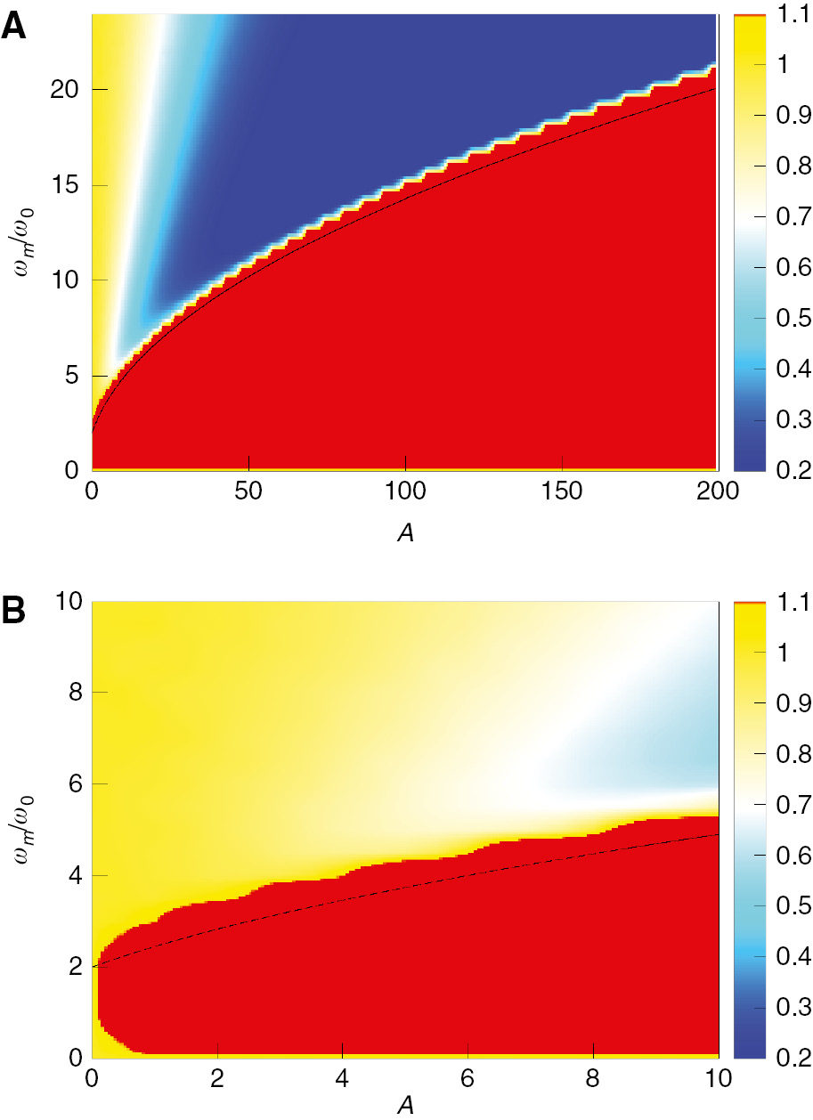
In Figure 1, we depict the time averaged variance 〈x(t)2〉, of the steady state of the driven system, as a function of A and ωm/ω0. Here, and in the examples throughout this article, we choose γ/ω0=0.1. The most striking feature of this plot is the parametric resonance that appears near ωm≈2ω0, for small A. This feature is then power broadened for increasing A. In this regime, the magnitude of 〈x(t)2〉 is increased by orders of magnitude, compared to the equilibrium value. In addition to this strong heating effect, there is a regime for large ωm/ω0, and large amplitude, for which a reduction of 〈x(t)2〉 is observed. Here, the parametric driving leads to a dynamic stabilisation of the fluctuations of x. It is this counterintuitive and quintessential example of reducing fluctuations via high-frequency driving that we study systematically in this article.
We depict the time averaged magnitude of
In Figure 2, we show the same quantity in the steady state as a function of A, for a fixed value of the driving frequency, ωm/ω0=20, to give a clearer insight into the quantitative behaviour. The magnitude of these fluctuations is visibly reduced with increasing driving amplitude. However, eventually this trend of decreasing fluctuations is rapidly reverted, resulting in a steep increase of the fluctuations. As visible from Figure 1, this steep increase is due to the power-broadened parametric instability. The onset of this instability determines the location of the minimal amount of fluctuations that can be achieved with this type of driving. It is therefore imperative to understand the origin of this steep increase of the fluctuations and provide a systematic approach to determine its behaviour.
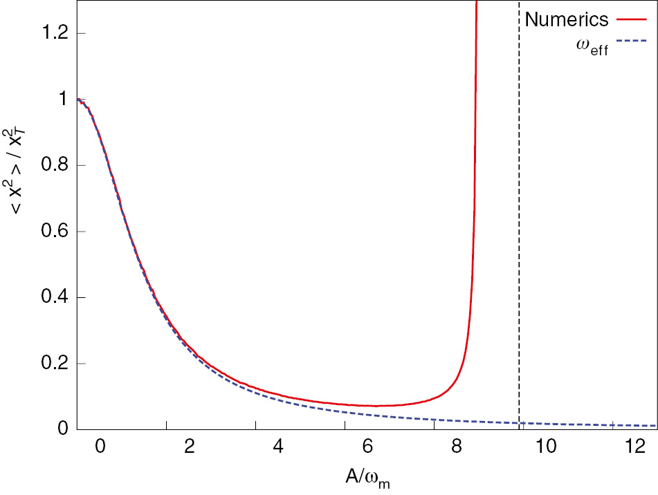
We depict the time averaged expectation value of 〈x2〉, in units of
In Figure 3, we show a histogram of the distribution ρdr in the steady state, in comparison to the equilibrium distribution ρ0; we show ρdr−ρ0. The distribution ρdr is generated from trajectories of the Langevin equation, which have been low-frequency filtered via
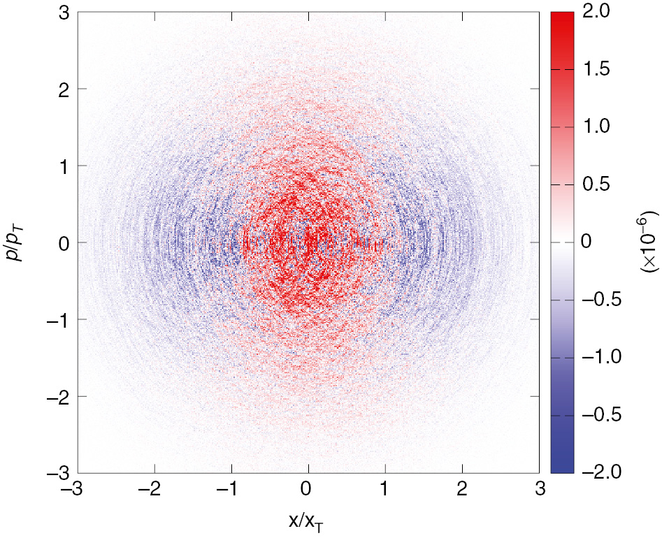
Distribution in phase space of the driven system in the steady state. The trajectories of the time evolution have been smoothed out on a time scale of σ=1/ω0. We use ωm/ω0=20, A=10, and γ/ω0=0.1. The binning size is Δx/xT=Δp/pT=0.01. The reduction of the width of the distribution in the x-direction is clearly visible.
2.1 Elementary Approach
Before we develop the renormalisation of the oscillator due to the periodic driving systematically in the following section, we give estimates of its behaviour using various ansatz functions.
We start out by giving an estimate for the instability regime, and note that a more detailed discussion is given in Appendix B. We consider the equation of motion of the isolated system,
The instability regime is reached when the expression under the outer square root becomes negative. This occurs at
which simplifies to
for large A. This provides an estimate for the instability regime for large driving amplitudes and frequencies, which we show in Figure 1, and which gives good agreement.
To give an estimate for the renormalisation of ωeff, we extend this ansatz to include not only the frequencies ωeff and ωm−ωeff, but also the next three contributing terms, corresponding to the frequencies ωm+ωeff, 2ωm−ωeff and 2ωm+ωeff. This ansatz is explicitly written in (B5). This ansatz results in (B6) for the effective frequency. We solve this equation iteratively in the amplitude A, which gives the expansion
At second order in A and at second order in the inverse driving frequency, this is
This approximation for the effective frequency is shown in Figure 2. We note that the fourth-order term in (9) is positive. This is indeed confirmed further down by the systematic Magnus expansion. However, the Magnus expansion determines the correct prefactor, which differs from the one found here.
3 Magnus Expansion
We now turn to the Magnus expansion of the system. This expansion provides a time-independent approximation of the low-frequency sector of the system, derived from the original, time-dependent Hamiltonian that describes all frequencies. After deriving general expressions for the Magnus terms beyond second order, we ask the question if and how the key features of the parametric oscillator, the dynamical stabilisation and the instability regime, can be captured within this approach. We note that these features, as they were described in the previous section, might suggest that such an approach might not be possible in a consistent fashion for the fourth-order correction. This is due to the following two observations. We observed, as shown in (9), that the fourth-order correction has a positive prefactor, which results in an addition stabilisation of the oscillator. This term would be derived from a term in an effective Hamiltonian that is of the form
Interestingly, as we discuss below, the Magnus expansion provides two types of terms at fourth order. One of them is cut-off independent and features a positive prefactor. The resulting renormalisation due to this term is in agreement with the numerically obtained result. The other term is cut-off dependent. It indicates that the hierarchy of time scales that is required for the Magnus expansion breaks down. We interpret this as a precursor of the instability regime, and indeed find that the scaling for this regime, as shown in (8), is predicted correctly.
3.1 Kramers Equation
To apply the Magnus expansion, we formulate the time evolution of the system (4 and 5), as a time evolution of the phase space distribution ρ(x, p, t). This is given by the Kramers equation
Here, L(t)=L0+Ldr(t) with
and
with
We refer to (11) as the Kramers equation to distinguish it from the Fokker–Planck equation, which we reserve for the over-damped limit, in accordance with the terminology of [22].
3.2 General Expansion
We now derive the expansion of the low-energy description in full generality. We consider a general, dynamical system that is described by the same equation of motion
as before, without the assumption of the specific form of the equation of motion, as in the previous section. The parametrically driven oscillator will serve as the example to which we apply our results further down. The system under consideration can be either a closed or an open classical system or a closed quantum system. For a closed quantum system, we interpret the operator L(t) as a Hamiltonian, divided by iћ, i.e. L(t)=H(t)/(iћ). For an open system, we also include dissipative terms, as in (11). We again assume that L(t) has the form
where L0 describes the time-independent part of the system and Ldr(t) is the driving term, again of the form
We perform the Magnus expansion in the interaction picture. In this picture, the order of the Magnus expansion coincides with the order of the driving term. In the case of the parametric oscillator, this is the order of the driving amplitude A. For the interaction picture, we define
where the standard interaction picture term is Ldr,i(t)=Ldr,i (t, t). Then the equation of motion is
Its solution is
where Tt is the time ordering operator and ρi(t0) the initial state at t0. The Magnus expansion consists of re-expressing this solution in the form
We time average each of these terms over a time interval [t0, t]. The time interval is long compared to the driving period but short compared to the dynamics that is created by H0. For the parametric oscillator, we demand 1/ω0≫t−t0≫1/ωm. The time interval Δtc=t−t0 is also the inverse of a frequency cut-off ωc=2π/Δtc, for which we equivalently demand ω0≪ωc≪ωm. For a general system, the frequency ω0 has to be replaced by a typical frequency that is characteristic for the dynamics of H0.
The second-order Magnus term in the interaction picture is given by
We transfer this expression back to the Schrödinger picture and project this term on the frequency range below ωc. The resulting effective
with
We use this first-order expansion, with
The low-frequency part of the time integral, which refers to frequencies below ωc, is
Therefore, we obtain
Here, and throughout the article, we use the notation
3.3 Fourth Order in ω m − 1
We now derive the next order term in the inverse frequency. We consider the expansion in (18) to third order
where we introduced the notation of the adjoint derivative
We use the integral property
which results in
Higher order terms of the form
3.4 Fourth-Order Magnus Expansion
For the fourth-order term in the driving term, we proceed along the same lines as for the quadratic term in the previous sections. The fourth-order term in the interaction picture has the form
Again, we transform this expression to the Schrödinger picture. We project this term on the low-frequency regime. Interestingly, we find two contributions, as we show below. The first is proportional to Δtc. Therefore, it lends itself to an interpretation as an effective low-energy description. The second term is cubic in Δtc, which means that we can write
and we also introduce the definition
with
The integrals that are necessary to derive
The value of the integrals of the form given in (33), which are necessary to evaluate (32) at order k=3.
| c0,0,3 | c0,1,2 | c0,2,1 | c0,3,0 | c1,0,2 | c1,2,0 | c2,0,1 | c2,1,0 | |
|---|---|---|---|---|---|---|---|---|
The term that scales as
We emphasise again that for any system that can be written in the form of (15–17), the results given in (26, 29, 34, and 35) apply. They constitute the main conceptual result of this paper.
4 Magnus Expansion of the Parametric Oscillator
We now apply our results to the case of the parametric oscillator, introduced above. For the
This implies a renormalisation of the oscillator frequency of the form
This coincides with the second-order term that was obtained in (10). At the fourth in the inverse driving frequency, we have
where we applied (29). Interestingly, in addition to a further renormalisation of the oscillator frequency, a renormalisation of the temperature is created:
It is generated because the white-noise dissipative term contains fluctuations at all frequencies, in particular at the driving frequency ωm. This results in an additional renormalisation of the low-frequency regime, via time averaging, of the system at this higher order. For the example presented here, the magnitude of the renormalisation is small. However, nonlinear systems will in general create nonlinear effective dissipative terms at this order. Finally, we determine the two terms at order A4. The cut-off independent term is
This term generates an additional renormalisation of the oscillator frequency, resulting in
We note that this renormalisation at fourth order in A has a positive prefactor, as in the estimate in (9). However, the systematic Magnus expansion gives the correct magnitude of the prefactor.
In Figure 4, we depict the power spectrum Sp(ω) of the momentum p in steady state, as a function of the driving amplitude A, and for the fixed driving frequency ωm/ω0=20. The power spectrum is defined via
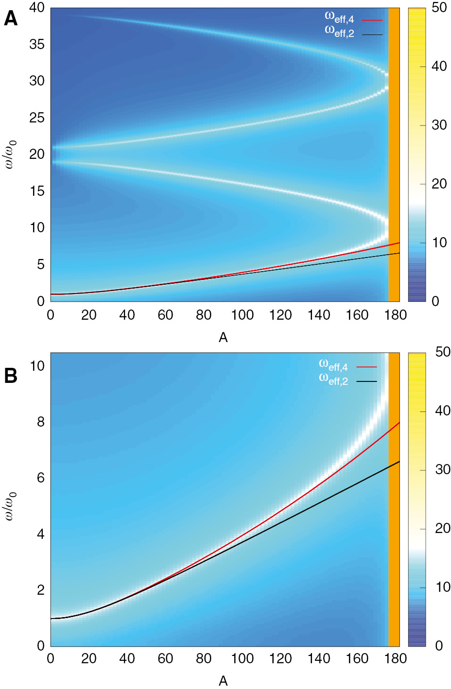
Power spectrum Sp(ω) as a function of the driving amplitude A, depicted on a logarithmic scale. For the driving frequency, we use ωm/ω0=20. We show the second-order estimate of the effective frequency, ωeff,2, which refers to (37). In addition, we show the fourth-order estimate ωeff,4, based on (42).
with
The cut-off dependent term is
This term competes with the previously discussed terms that stabilise the oscillator. For simplicity, we only consider the dominant term of the effective frequency (36). We relate the time scale Δtc to a frequency cut-off via Δtc=2π/ωc. We assume to be in the strongly renormalised regime,
This results in the criterium
If we consider a cut-off frequency chosen as fraction of the driving frequency, and therefore ωc~ωm, we recover
which displays the same scaling as in (8). The scaling displayed in (46) can also be motivated by comparing the cut-off frequency ωc to ωeff/ω0~Aω0/ωm. Again, this condition indicates that the originally assumed hierarchy of energy scales is no longer valid. This property of the system derives from the cut-off dependent term
5 Parametrically Driven Chain
We apply this formalism to the stabilisation of a chain of oscillators via parametric driving. This, and related mechanisms have been considered in the context of light enhanced superconductivity, with the following motivation. If we imagine a complex order parameter field describing fluctuating superconducting order, a key feature of this system is its phase stiffness. In equilibrium, it controls the superconducting stability and the critical current. The phase stiffness in turn is related to how steeply the dispersion of the system increases with increasing momentum. Therefore, one possible explanation of light enhanced superconductivity might entail stabilising and steepening the dispersion of the system.
We here give the simplest, yet generic, case of a one-dimensional chain of oscillators. The system is described by H=H0+Hdr(t), with
with i=1, …,N. The driving term is
We therefore have a parametrically driven lattice of oscillators. We Fourier transform the system via
with
We observe that (50 and 51) are equivalent to (4 and 5), with the replacement ω0→ωk,0. We can therefore apply the results for the single oscillator (42), to each momentum mode and obtain the effective dispersion
The second-order correction, derived from
In Figure 5, we show the two point correlation Γ(k, ω) in momentum and coordinate space in the steady state for a one-dimensional chain of parametrically driven oscillators. The two point correlation function is defined by
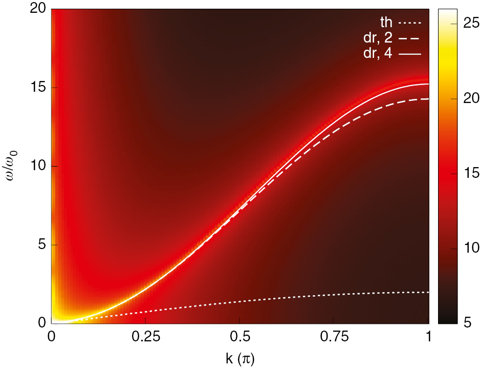
Two-point correlation function 𝒢(k, ω), depicted on a logarithmic scale. We use ωm/ω0=80 for the driving frequency with driving amplitude A=400. We compare the numerics with the analytical estimates (white lines), respectively, thermal situation (dotted line), second-order estimate (dashed line), and fourth-order estimate (solid line) of the effective frequency, ωk,eff, which refers to (53).
with
where Ts and Ks are sampling time interval and space interval, respectively. Compared with the nondriven situation, the driven dispersion line has a steeper slope, which means that the driving term stiffens the system significantly. We compare the numerics with effective dispersion ωk,eff, (53). It is clearly seen that at higher k modes, the second-order correction deviates from the numerics while the fourth-order correction describes the numerics precisely.
We also observe that the strongest renormalisation of the dispersion occurs at its upper edge. This includes the onset of the parametric instability. We now have the condition
which is first reached for the maximum of the band. This sets the upper limit for the driving amplitude A that can be used to stabilise the dispersion. However, we note that, depending on the physical system, the range of A might be much more limited. For example, the value of the spring constant between neighboring oscillators might not allow for negative values, meaning that A<1. With this constraint, the magnitude of the renormalisation is small, of the order of
6 Conclusions
We have developed a systematic Magnus expansion in the driving term and the inverse driving frequency. In this formalism, we have derived explicit expressions for a system with a driving term with cosine time dependence. This system can be either a quantum mechanical system or a classical system including dissipative terms. The main, conceptual formulas are given in (29, 34, and 35), which are the terms beyond the widely discussed lowest order term in (26). At fourth order in the driving term, we find two contributions, one cut-off independent and one cut-off dependent. The cut-off independent term contributes to the effective Kramers or Hamilton operator, whereas the increasing magnitude of the cut-off dependent term indicates the breakdown of the hierarchy of time scales that was originally assumed. We apply this formalism to a parametrically driven oscillator, coupled to a thermal bath, and to a parametric oscillator chain. We obtain the magnitude of stabilisation that can be achieved for these systems and the onset of the instability. We emphasise that our formalism can be applied to a wide range of driven systems, including nonlinear systems and many-body systems. It will be of particular interest to the emerging field of controlling many-body systems via external driving.
Acknowledgements
We gratefully acknowledge discussions with Andrea Cavalleri, Robert Höppner, and Junichi Okamoto. We acknowledge support from the Deutsche Forschungsgemeinschaft through the SFB 925 and through Project No. MA 5900/1-1, the Hamburg Centre for Ultrafast Imaging, and from the Landesexzellenzinitiative Hamburg, supported by the Joachim Herz Stiftung. B.Z. acknowledges support from the China Scholarship Council, under scholarship No. 2012 0614 0012.
Appendix A: Frequency Cut-Off
In this section, we discuss the comparison of the predictions of the effective description to the observables extracted from the full system. Because the effective description is a low-frequency description, it is, in general, imperative to apply a frequency cut-off on the observables, for a quantitative comparison. While for some observables depend only weakly on the introduction of this cut-off, in general, the low-pass-filtered observable will differ from the observable that includes all frequencies.
As discussed in Section 2, we have depicted the phase space distribution that is derived from the low-frequency-filtered trajectories (xc(t), pc(t)) in Figure 3. For comparison, we depict the phase space distribution that is derived from original trajectories (x(t), p(t)) that include all frequencies, in Figure 6. As is clearly visible, for this distribution a broadening of the distribution in the p-direction occurs, in contrast to Figure 3.
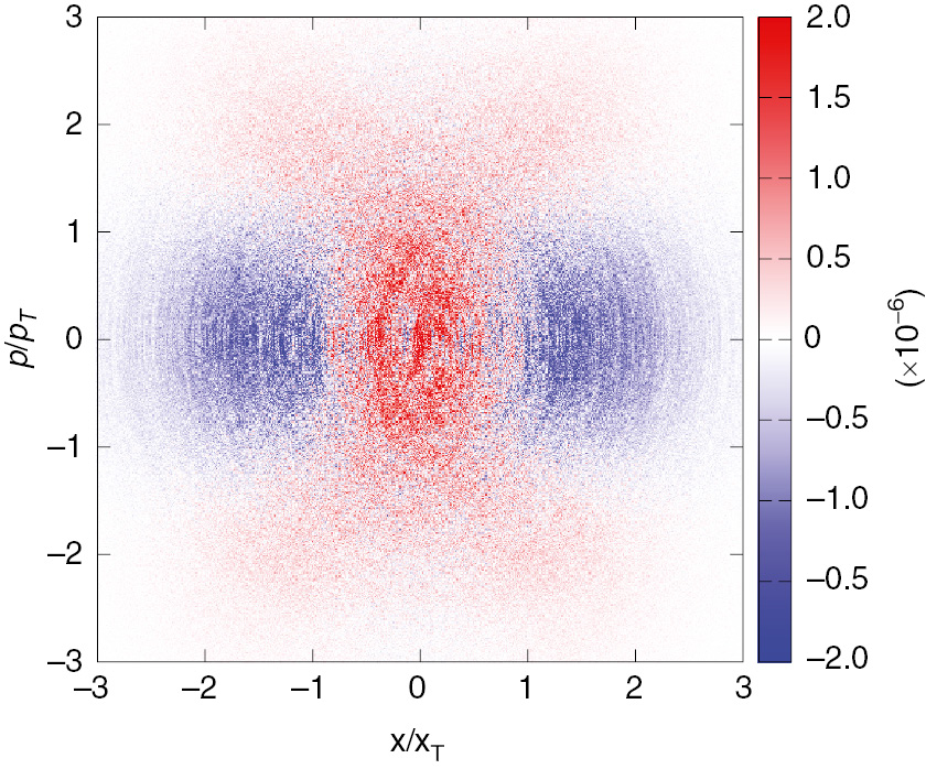
Distribution in phase space of the driven system in the steady state, for the same parameters as in Figure 3, but without the low-frequency filtering. For this distribution, an increase in the width in the p-direction is observed, which is due to high-frequency contributions.
To elaborate on this further, we depict the time average of 〈pc(t)2〉 and 〈p(t)2〉 in the steady state, as a function of A, in Figure 7. 〈p(t)2〉 has a strong dependence on A, which is approximately quadratic. 〈pc(t)2〉, however, has only a very weak A dependence, only given the weak temperature renormalisation that was given in (40).
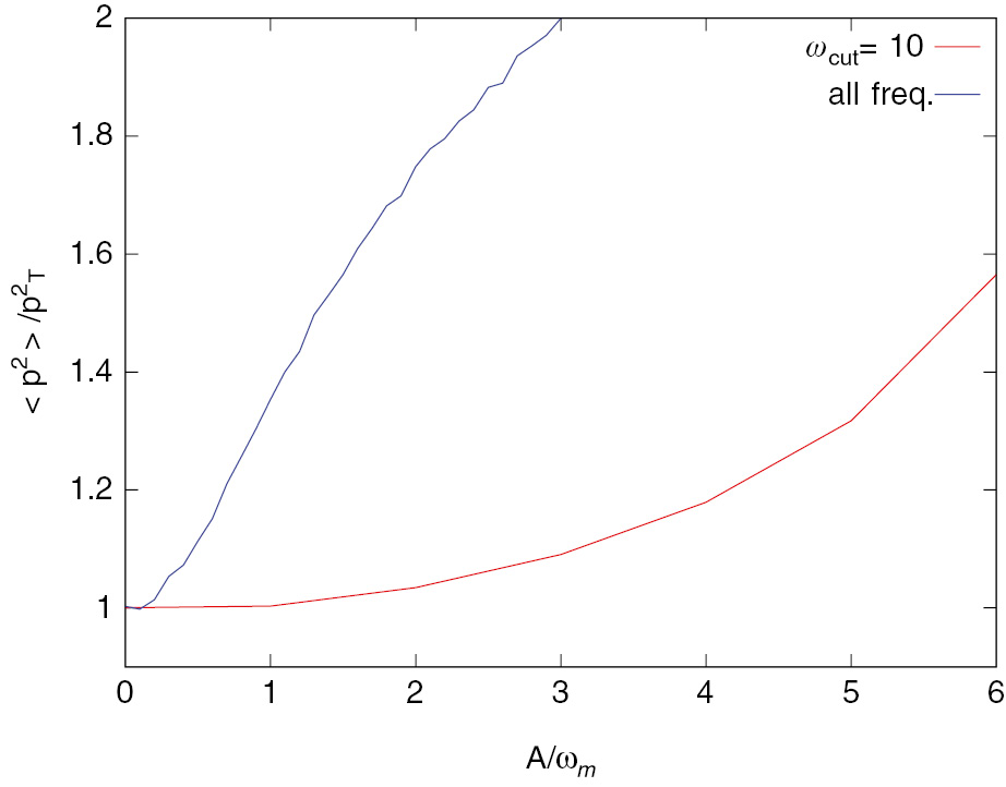
Time average value of p2(t), shown as the blue line, and
Appendix B: Elementary Ansatz
We consider the equation of motion for the isolated system
To estimate the regime in which the instability of the system occurs, we consider the ansatz
where a0 and a1 are constant coefficients. ωeff is the effective oscillation frequency, which we solve for. Substituting this ansatz in the equation of motion, and ignoring further frequencies, this results in the equations
The resulting ωeff is
The parametric resonance is reached when the expression under the square root becomes negative. We note that the effective frequency ωeff increases monotonously, with increasing A. The instability occurs when the two frequencies ωeff and ωm−ωeff equal each other. We confirm this behaviour by calculating the power spectrum of the driven state, which is shown in Figure 4.
To give a more accurate estimate of the renormalisation of ωeff, we consider the following ansatz
When we substitute this in the equation of motion, we obtain the following equation for ωeff:
We solve this equation iteratively in the driving amplitude A, which gives
Here, we kept the leading order in the inverse frequency 1/ωm for the fourth-order term, which scales as
Appendix C: Fourth-Order Term of the Magnus Expansion
After expanding (32) to the order k=3, evaluating the integrals of the form of (33), and collecting the terms that scale as
To simplify this expression, we first combine the terms that are related by commutation. In addition, we use that
and
With these identities, we simplify the expression to the form given in (34).
References
[1] J. Struck, M. Weinberg, C. Ölschläger, P. Windpassinger, J. Simonet, et al., Nat. Phys. 9, 738 (2013).10.1038/nphys2750Suche in Google Scholar
[2] C. Giannetti, M. Capone, D. Fausti, M. Fabrizio, F. Parmigiani, et al., Adv. Phys. 65, 58 (2016).10.1080/00018732.2016.1194044Suche in Google Scholar
[3] W. Hu, S. Kaiser, D. Nicoletti, C. R. Hunt, I. Gierz, et al., Nat. Mater. 13, 705 (2014).10.1038/nmat3963Suche in Google Scholar PubMed
[4] R. Mankowsky, A. Subedi, M. Först, S. O. Mariager, M. Chollet, et al., Nature 516, 71 (2014).10.1038/nature13875Suche in Google Scholar PubMed
[5] I. Gierz, J. C. Petersen, M. Mitrano, C. Cacho, E. Turcu, et al., Nat. Mater. 12, 1119 (2013).10.1038/nmat3757Suche in Google Scholar PubMed
[6] R. Höppner, B. Zhu, T. Rexin, A. Cavalleri, and L. Mathey, Phys. Rev. B 91, 104507 (2015).10.1103/PhysRevB.91.104507Suche in Google Scholar
[7] J.-i. Okamoto, A. Cavalleri, and L. Mathey, arXiv:1606.09276.Suche in Google Scholar
[8] M. A. Sentef, A. F. Kemper, A. Georges, and C. Kollath, Phys. Rev. B 93, 144506 (2016).10.1103/PhysRevB.93.144506Suche in Google Scholar
[9] Z. M. Raines, V. Stanev, and V. M. Galitski, Phys. Rev. B 91, 184506 (2015).10.1103/PhysRevB.91.184506Suche in Google Scholar
[10] S. J. Denny, S. R. Clark, Y. Laplace, A. Cavalleri, and D. Jaksch, Phys. Rev. Lett. 114, 137001 (2015).10.1103/PhysRevLett.114.137001Suche in Google Scholar PubMed
[11] A. A. Patel and A. Eberlein, Phys. Rev. B 93, 195139 (2016).10.1103/PhysRevB.93.195139Suche in Google Scholar
[12] L. D. Landau and E. M. Lifshitz, Mechanics Vol. 1 (1st ed.), Pergamon Press, Headington Hill Hall, Oxford 1960.Suche in Google Scholar
[13] W. Magnus, Commun. Pure Appl. Math. 7, 649 (1954).10.1002/cpa.3160070404Suche in Google Scholar
[14] S. Blanes, F. Casas, J. A. Oteo, and J. Ros, Phys. Rep. 470, 151 (2009).10.1016/j.physrep.2008.11.001Suche in Google Scholar
[15] W. R. Salzman, J. Chem. Phys. 82, 822 (1985).10.1063/1.448508Suche in Google Scholar
[16] L. D’Alessio and A. Polkovnikov, Ann. Phys. 333, 19 (2013).10.1016/j.aop.2013.02.011Suche in Google Scholar
[17] C. Zerbe, P. Jung, and P. Hänggi, Phys. Rev. E 49, 3626 (1994).10.1103/PhysRevE.49.3626Suche in Google Scholar PubMed
[18] C. Zerbe and P. Hänggi, Phys. Rev. E 52, 1533 (1995).10.1103/PhysRevE.52.1533Suche in Google Scholar PubMed
[19] E. I. Butikov, J. Phys. A 35, 6209 (2002).10.1088/0305-4470/35/30/301Suche in Google Scholar
[20] E. I. Butikov, Regular and Chaotic Motions of the Parametrically Forced Pendulum: Theory and Simulations, Springer Berlin, Heidelberg 2002.10.1007/3-540-47789-6_122Suche in Google Scholar
[21] M. G. Clerc, C. Falcón, C. Fernández-Oto, and E. Tirapegui, Europephys. Lett. 98, 30006 (2012).10.1209/0295-5075/98/30006Suche in Google Scholar
[22] N. G. van Kampen, Stochastic Processes in Physics and Chemistry, Elsevier, Amsterdam, Netherlands 1992.Suche in Google Scholar
©2016 Walter de Gruyter GmbH, Berlin/Boston
Artikel in diesem Heft
- Frontmatter
- Editorial
- Emergence in Driven Solid-State and Cold-Atom Systems
- Research Articles Focus Section
- Entropy Production Within a Pulsed Bose–Einstein Condensate
- Anatomy of a Periodically Driven p-Wave Superconductor
- Quasi-Periodically Driven Quantum Systems
- Interband Heating Processes in a Periodically Driven Optical Lattice
- Magnus Expansion Approach to Parametric Oscillator Systems in a Thermal Bath
- Research Articles
- The Extended C-Type of KP Hierarchy: Non-Auto Darboux Transformation and Solutions
- A Transverse Dynamic Deflection Model for Thin Plate Made of Saturated Porous Materials
- Accreting Scalar-Field Models of Dark Energy Onto Morris-Thorne Wormhole
- Rogue Wave and Breather Structures with “High Frequency” and “Low Frequency” in 𝒫𝒯-Symmetric Nonlinear Couplers with Gain and Loss
- Multimode Characteristics of Space-Charge Waves in a Plasma Waveguide