The Integrability of an Extended Fifth-Order KdV Equation in 2+1 Dimensions: Painlevé Property, Lax Pair, Conservation Laws, and Soliton Interactions

1 Introduction

In the past decades, many powerful methods to solve integrable systems, such as the inverse scattering transformations (ISTs), Darboux transformations, Bäcklund transformations (BTs), symmetry reduction, Hirota bilinear method, and Painlevé analysis method, have been developed [1]. The usual real physical nonlinear systems can be treated as perturbations of the related integrable models. It is an interesting task to generate new integrable equations in the soliton theory.

Painlevé analysis method has been identified as one of the most effective tools in studying nonlinear evolution equations (NLEEs) [2]. This analysis not only can verify whether a given equation possesses the Painlevé property, but it also can search for all possible integrable cases of a NLEEs with general forms [3–9]. Moreover, the remarkable feature of Painlevé analysis is that a natural connection exists in relation to many integrable properties such as Hirota bilinear forms, Lax pairs, BTs, and various types of exact solutions [10–15]. Hirota bilinear method is a direct method to derive the multiple-soliton solutions, quasi-periodic wave solutions, bilinear BT, and other properties of a given NLEEs [16–19]. The crucial step of this method relies on a particular skill by choosing suitable variable transformations, but there is no general rule to find the transformations. Using the links between the Bell polynomials and Hirota D-operators, Lambert and his coworkers have established a direct method to derive bilinear forms, bilinear BT and Lax pairs of soliton equations systematically [20, 21]. The Bell polynomials approach has been extended to the variable-coefficient, supersymmetric, and discrete NLEEs [22–39].

In this work, we will employ the Painlevé analysis and Bell polynomial method to study an extended fifth-order Korteweg–de Vries (KdV) equation

which is an important higher-order extension of the famous KdV equation in fluid dynamics. The KdV-type equations have been widely recognized as ubiquitous mathematical models for describing some nonlinear phenomena in many branches o f physics. The higher-order dispersion and nonlinear terms must be taken into account in some complicated situations such as the surface and internal waves, gravity–capillary waves, longitudinal waves in microstructured solids, and so on. In (1), u=u(x, y, t) and λ_j(j=1, …, 8) are real parameters. Much research has been done for its particular cases. However, the integrability of the generalized equation (1) has not been investigated.

Equation (1) includes a number of important NLEEs as its special cases. Konopelchenko and colleagues [40, 41] constructed and studied two integrable equations:

which are the (2+1)-dimensional integrable generalization of the Sawada–Kotera (SK) equation and the Kaup–Kuperschmidt (KK) equation, respectively. The Lax pair, conservation laws, symmetry structure, and multiple-soliton solutions of (2) and (3) have been investigated in [42–44].

When λ₁=1/36, λ₂=λ₃=5/12, λ₄=5/4, λ₅=λ₆=–5/36, λ₇=λ₈=–5/12, (1) reduces to the (2+1)-dimensional Caudrey–Dodd–Gibbon–Kotera–Sawada equation:

Its symmetry constraints and quasi-periodic solutions have been constructed [45, 46].

When λ₁=1/9, λ₂=5/3, λ₃=25/6, λ₄=5, λ₅=–λ₆=–5σ/9, λ₇=λ₈=5σ/3, (1) reduces to the (2+1)-dimensional KK equation with another form:

Its multiple-soliton solutions and symmetry algebras have been presented [47].

Using gauge transformation, He and Li [48] studied two other particular cases of (1):

Up to now, we have already known that (2)–(7) are integrable. The natural and important question is under what constraints on parameters λ_j (j=1, …, 8) is (1) integrable, i.e. does another new integrable subcase of (1) exist? In the following section, we will perform the Painlevé test for the extended equation (1) to derive all possible integrable subcases. In Section 3, by employing the Bell polynomials method, we systematically construct the bilinear forms, bilinear BT and Lax pair for the new integrable equation. In Section 4, the N-soliton solutions and their collisions are discussed. Some conclusions are given in the final section.

2 Integrability Test

To verify whether a given NLEEs possesses the Painlevé property, one may use different methods, such as the Weiss–Tabor–Carnevale (WTC) method, Kruskal’s simplification for the WTC method, Conte invariant method, Lou’s extended method, and so on. Here we apply the WTC–Kruskal’s approach to carry out the Painlevé integrability test for (1). Taking u_y=v_x, (1) becomes the following coupled system:

(8)ut + λ1uxxxxx + λ2uuxxx + λ3uxuxx + λ4u2ux + λ5uxxy + λ6vy  + λ7uuy + λ8uxv = 0,uy = vx. (8)

To simplify the calculations, the Kruskal’s ansatz ϕ(x, y, t)=x+ψ(y, t) is adopted here.

Inserting u(x, y, t) = u0ϕα1, v(x, y, t) = v0ϕα2 into the leading terms of (8), we have

To determine the resonant points, we set

u(x, y, t) = u0ϕ−2 + ujϕj − 2, v(x, y, t) = v0ϕ−2 + vjϕj − 2,  uj = uj(y, t), vj = vj(y, t).

Substituting the truncated expansions into the dominant terms of (8) yields a polynomial equation in j,

where u₀ is given by (9). From (10), we know that three resonant points occur at –1, 2, 6. Other three undetermined resonances, say j₁, j₂, j₃, must be integers, and this is possible if

Solving the first equation of (11) yields j₃=15–j₁–j₂. The considered branch should be generic, i.e. five resonant points lie in positive integer positions. Then the positive integer conditions for j₁, j₂, j₃ result in 16 different subcases: (1) [1, 1, 13], (2) [1, 2, 12], (3) [1, 3, 11], (4) [1, 4, 10], (5) [1, 5, 9], (6) [1, 6, 8] (7) [1, 7, 7], (8) [2, 3, 10], (9) [2, 4, 9], (10) [2, 5, 8], (11) [2, 6, 7], (12) [3, 3, 9], (13) [3, 4, 8], (14) [3, 5, 7], (15) [4, 4, 7], (16) [4, 5, 6].

Testing all the resonant conditions for subcases (1)–(16) yields possible Painlevé integrable models under some constraints on parameters λ_j. For instance, for case (10), solving (9) and (11) with respect to λ₁, λ₂, λ₃, u₀, and v₀ will lead to

Six resonant points occur at –1, 2, 2, 5, 6, 8. To test the resonant conditions, one may take

Inserting expansions (13) into (8) and setting the coefficients of {ϕ⁻⁶, ϕ⁻²} to zero, we get u₁=v₁=0.

For j=2, collecting the coefficients of {ϕ⁻⁵, ϕ⁻¹} will lead to

where parameter λ₁ cannot be taken as zero, thus condition (14) is satisfied if and only if

For j=3 and j=4, setting the coefficients of {ϕ⁻⁴, ϕ⁰} and {ϕ⁻³, ϕ¹} to zero, we get

u3 = 0, v3 = u2,y, u4 = 40λ1(λ6ψy2 + λ7u2ψy + ψt − λ7v2) + 3λ3(λ3u22 + 4λ5)40λ1λ3, v4 = u4ψy.

For j=5, the corresponding resonant condition is obtained as

where parameter λ₁ cannot be taken as zero; thus, condition (16) is consistent if and only if

Together with conditions (12), (15), and (17), the final parametric constraints read

Under constraints (18), the coefficients u₂, v₂, u₅, u₆, u₈, ψ in (13) are arbitrary functions of {y, t}, which indicate that the conditions at all non-negative resonant points are verified and the remaining coefficients in (13) are

u1 = v1 = u3 = 0, v3 = u2,y, u4 = 3λ32u22 + 8λ3λ5u2ψy + 40λ1ψt + 4λ3λ5v240λ1λ3, v4 = u4ψy,u7 = λ3λ5u2u2,y + 5λ1(u2,t − 14λ5u5ψy − 3λ3u2u5 − 6λ5u4,y + 8λ5v5)400λ12,v5 = u5ψy + u4,y3,   v6 = u6ψy + u5,y4,   v7 = u6,y5 + u7ψy,   v8 = u7,y6 + u8ψy.

Under parameter constraints (18), there is another secondary branch for (8). For the secondary branch, the leading order analysis leads to α₁=α₂=–2, u₀=–40λ₁/λ₃, v₀=–40λ₁ψ_y/λ₃. Six resonant points occur at –3, –1, 2, 6, 8, and 10. To verify the resonant conditions, we suppose

Substituting it into (8) and collecting the different powers of ϕ will lead to

u1 = v1 = u3 = u5 = 0, u2 = − λ5ψy2λ3, v3 = u2,y, u4 = 10λ1ψt − λ52ψy2 + λ3λ5v270λ1λ3, v4 = u4ψy,   v5 = u4,y3, v6 = u6ψy, u7 = λ5(20λ1ψyt + λ3λ5v2,y − 6λ52ψyψyy)1200λ12λ3,   v7 = u6,y5 + u7ψy,   v8 = u8ψy + u7,y6,u9 = 5λ1(u4,t − 24λ3u2u7) + λ3λ5(v3u4 + u2u4,y + u4u2,y) − 60λ1λ5(u6,y + 6u7ψy − 2v7)1800λ12,   v9 = u8,y7 + u9ψy,   v10 = u9,y8 + u10ψy,

where the coefficients v₂, u₆, u₈, u₁₀ in (19) are arbitrary functions of {y, t}.

The above analysis for case (10) yields the first type of integrable model.

Integrable model I (new integrable model):

where parameters λ₁ and λ₃ are arbitrary nonzero constants.

Performing the similar analysis for other cases, one can obtain other two integrable subcases of (1). For simplicity, the detailed computations are omitted.

Integrable model II (2+1-dimensional generalized SK equation):

where parameters λ₁ and λ₃ are arbitrary nonzero constants. For model (21), there is a primary branch with the resonances located at {–1, 2, 2, 3, 6, 10} and a secondary branch with the resonances located at {–2, –1, 2, 5, 6, 12}, and all the resonant conditions are consistent.

Integrable model III (2+1-dimensional generalized KK equation):

where parameters λ₁ and λ₃ are arbitrary nonzero constants. For model (22), there is a primary branch with the resonances located at {–1, 2, 3, 6, 7} and a secondary branch with the resonances located at {–7, –1, 2, 6, 10, 12}, and all the resonant conditions are consistent.

If we take appropriate values for λ_j (j=1, 3, 5), (21) and (22) can be reduced to the particular cases (2)–(7), which are exactly the 2+1-dimensional integrable generalizations of the SK and KK equations, respectively. Equation (20) is a new fifth-order integrable model in 2+1 dimensions and has not been reported in literature.

3 Bell Polynomials Method for (20)

In this section, we will employ the Bell polynomials method to study the new integrable equation (20).

4 Interactions of Multiple Solitons

From (28), the one-soliton solution reads

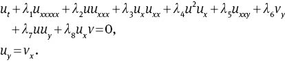
where parameters k₁, l₁, and ξ₀ are arbitrary constants. The profile of the one-soliton via solution (41) is shown in Figure 1. It can be seen that the soliton amplitude increases with the increase of k₁ while other parameters are fixed.

Figure 1:

One soliton given by expression (41) with λ₁=2.2, λ₃=7.6, λ₅=2, l₁=0.8, ξ₁₀=0.

The two-soliton solution can be written as

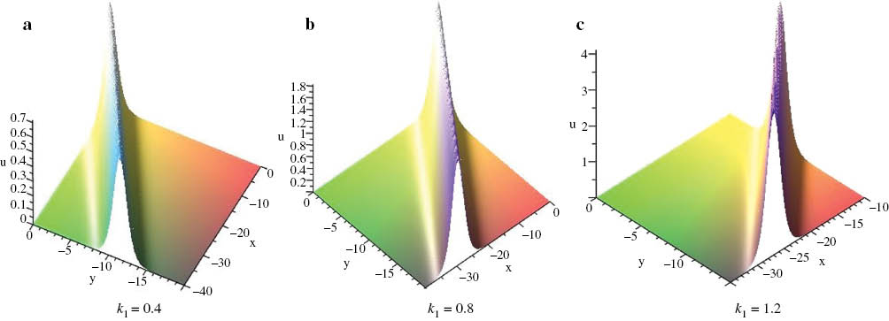
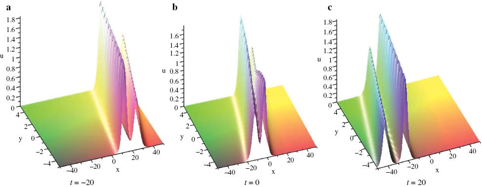
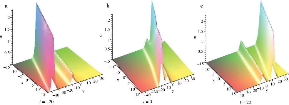
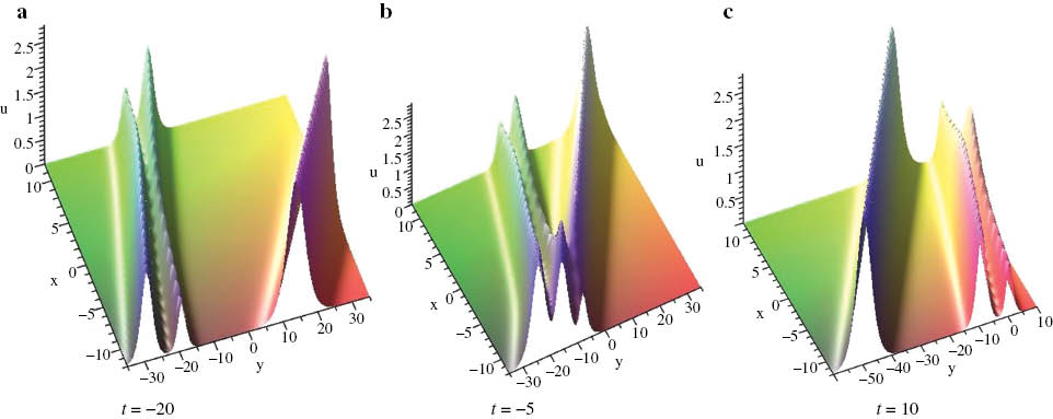
By selecting appropriate parameter values via solution (42), four different types of collisions of two solitary waves are shown in Figures 2–5. Elastic overtaking collisions of two solitary waves are illustrated in shown in Figures 2 and 3. Figure 2 show that two solitary waves are left-going along the x-axis and the smaller-amplitude soliton moves faster and then overtakes the larger. After the collision, the wave shapes and velocities remain unchanged. Figure 3 shows that two solitary waves are right-going along the y-axis and the larger-amplitude soliton overtakes the smaller one. The head-on collision of two solitary waves along opposite directions is depicted in Figure 4. When k₁=k₂, l₁≠l₂, V-type collisions occur, as shown in Figure 5.

Figure 2:

The overtaking collision of two solitary waves given by (42), where λ₁=2.2, λ₃=7.6, λ₅=2, k₁=0.6, k₂=0.8, l₁=–1.5, l₂=–1.2, ξ₁₀=ξ₂₀=0.

Figure 3:

The overtaking collision of two solitary waves given by (42), where λ₁=2.2, λ₃=7.6, λ₅=2, k₁=0.6, k₂=0.9, l₁=0.8, l₂=1.0, ξ₁₀=ξ₂₀=0.

Figure 4:

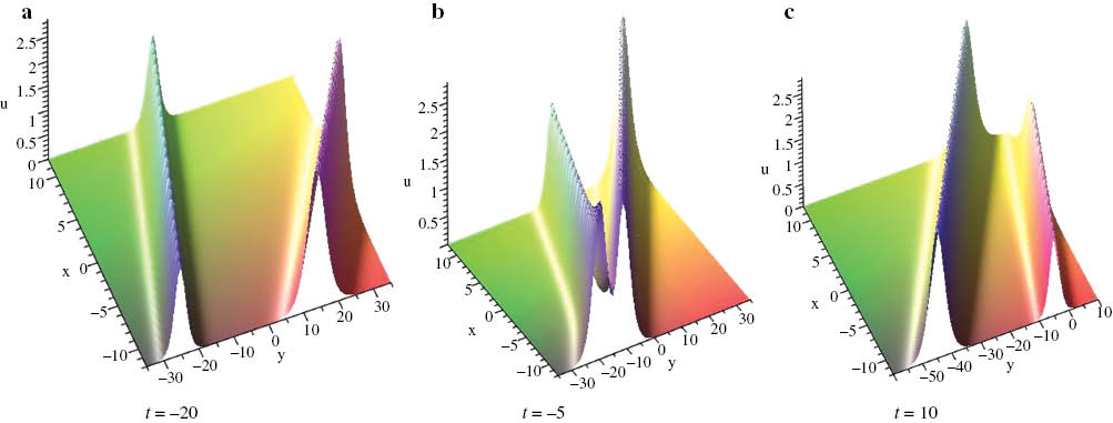
The headon collision of two solitary waves given by (42), where λ₁=2.2, λ₃=7.6, λ₅=2, k₁=1.0, k₂=0.6, l₁=–0.5, l₂=–1.5, ξ₁₀=ξ₂₀=0.

Figure 5:

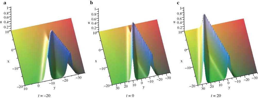
The V-type collision of two solitary waves given by (42), where λ₁=2.2, λ₃=7.6, λ₅=2, k₁=k₂=0.6, l₁=–1.15, l₂=–0.9, ξ₁₀=ξ₂₀=0.

More interesting collisions of three solitary wave can be exhibited by graphs. For the sake of simplicity, here, only the overtaking collisions and head-on collisions are shown in Figures 6 and 7, respectively.

Figure 6:

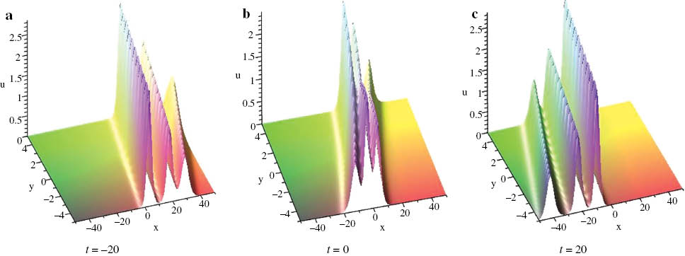
The overtaking collision of three solitary waves given by (28), where N=3, λ₁=2.2, λ₃=7.6, λ₅=2, k₁=0.6, k₂=0.8, k₃=1.0, l₁=–1.5, l₂=–1.2, l₂=–1.35, ξ₁₀=ξ₂₀=ξ₃₀=0.

Figure 7:

The head-on collision of three solitary waves given by (28), where N=3, λ₁=2.2, λ₃=7.6, λ₅=2, k₁=0.8, k₂=1.0, k₃=0.6, l₁=–0.1, l₂=–0.5, l₃=–1.5, ξ₁₀=ξ₂₀=ξ₃₀=0.

5 Conclusions

Using the WTC–Kruskal method and symbolic computation, we performed the Painlevé test for an extended 2+1-dimensional fifth-order KdV equation. Three distinct cases that pass the Painlevé test have been found, and two of those cases correspond to the generalizations of the integrable equations (2)–(7), whereas the first one turns out to be new.

For the new integrable model (20), we employed the Bell polynomials method to further prove its integrability. As a result, we derived the bilinear forms, bilinear BT, Lax pair, and infinite conservation laws systematically. Moreover, we also obtained the N-soliton solutions of the new obtained model. The collisions of multiple solitons have been discussed, which include overtaking, head-on as well as V-type collisions. Further studies on other integrable properties and exact solutions of this new unnamed model should be done in the future.

References

[1] M. J. Ablowitz and P. A. Clarkson, Solitons, Nonlinear Evolution Equations and Inverse Scattering, Cambridge University Press, Cambridge 1991.10.1017/CBO9780511623998Suche in Google Scholar
[2] J. Weiss, M. Tabor, and G. Carnevale, J. Math. Phys. 24, 522 (1983).10.1063/1.525721Suche in Google Scholar
[3] W. H. Steeb and N. Euler, Nonlinear Evolution Equations and Painlevé Test, World Scientific, Singapore 1988.10.1142/0723Suche in Google Scholar
[4] G. Q. Xu and Z. B. Li, Comput. Phys. Commun. 161, 65 (2004).10.1016/j.cpc.2004.04.005Suche in Google Scholar
[5] G. Q. Xu, Phys. Rev. E 74, 027602 (2006).10.1103/PhysRevE.74.027602Suche in Google Scholar PubMed
[6] G. Q. Xu, Comput. Phys. Commun. 178, 505 (2008).10.1016/j.cpc.2007.11.006Suche in Google Scholar
[7] G. Q. Xu, Comput. Phys. Commun. 180, 1137 (2009).10.1016/j.cpc.2009.01.019Suche in Google Scholar
[8] G. Q. Xu, Chin. Phys. B 22, 050203 (2013).10.1088/1674-1056/22/5/050203Suche in Google Scholar
[9] G. Q. Xu, Phys. Scripta 89, 125201 (2014).10.1088/0031-8949/89/12/125201Suche in Google Scholar
[10] A. Pickering, J. Phys. A: Math. Gen. 26, 4395 (1993).10.1088/0305-4470/26/17/044Suche in Google Scholar
[11] A. Pickering, J. Math. Phys. 35, 821 (1994).10.1063/1.530615Suche in Google Scholar
[12] S. Y. Lou, Z. Naturforsch. 53a, 251 (1998).10.1515/zna-1998-0523Suche in Google Scholar
[13] X. P. Cheng, C. L. Chen, and S. Y. Lou, Wave motion 51, 1298 (2014).10.1016/j.wavemoti.2014.07.012Suche in Google Scholar
[14] S. Y. Lou, Stud. Appl. Math. 134, 372 (2015).10.1111/sapm.12072Suche in Google Scholar
[15] Y. J. Ye, D. D. Zhang, and Y. M. Di, Z. Naturforsch. 70a, 823 (2015).10.1515/zna-2015-0248Suche in Google Scholar
[16] R. Hirota, The Direct Method in Soliton Theory, Cambridge University Press, Cambridge 2004.10.1017/CBO9780511543043Suche in Google Scholar
[17] S. F. Deng, Phys. Lett. A 362, 198 (2007).10.1016/j.physleta.2006.10.008Suche in Google Scholar
[18] S. F. Deng and Z. Y. Qin, Phys. Lett. A 372, 5426 (2008).10.1016/j.physleta.2008.06.052Suche in Google Scholar
[19] S. F. Deng, Appl. Math. Comput. 218, 5974 (2012).10.1016/j.amc.2011.11.076Suche in Google Scholar
[20] F. Lambert, I. Loris, and J. Springael, Inverse Probl. 17, 1067 (2001).10.1088/0266-5611/17/4/333Suche in Google Scholar
[21] F. Lambert and J. Springael, Acta Appl. Math. 102, 147 (2008).10.1007/s10440-008-9209-3Suche in Google Scholar
[22] E. G. Fan, Phys. Lett. A 375, 493 (2011).10.1016/j.physleta.2010.11.038Suche in Google Scholar
[23] E. G. Fan, Stud. Appl. Math. 127, 284 (2011).10.1111/j.1467-9590.2011.00520.xSuche in Google Scholar
[24] E. G. Fan and Y. C. Hon, J. Math. Phys. 53, 013503 (2012).10.1063/1.3673275Suche in Google Scholar
[25] Y. Zhang, W. W. Wei, T. F. Cheng and Y. Song, Chin. Phys. B 20, 110204 (2011).10.1088/1674-1056/20/11/110204Suche in Google Scholar
[26] W. X. Ma, Front. Math. China 8, 1139 (2013).10.1007/s11464-013-0319-5Suche in Google Scholar
[27] W. X. Ma, Rep. Math. Phys. 72, 41 (2013).10.1016/S0034-4877(14)60003-3Suche in Google Scholar
[28] Y. F. Zhang and H. Tam, J. Math. Phys. 54, 013516 (2013).10.1063/1.4788665Suche in Google Scholar
[29] Y. F. Zhang, Z. Hang, H. Tam, Commun. Theor. Phys. 59, 671 (2013).10.1088/0253-6102/59/6/03Suche in Google Scholar
[30] Y. H. Wang and Y. Chen, J. Math. Anal. Appl. 400, 624 (2013).10.1016/j.jmaa.2012.11.028Suche in Google Scholar
[31] Q. Miao, Y. H. Wang, Y. Chen, and Y. Q. Yang, Comput. Phys. Commun. 185, 357 (2014).10.1016/j.cpc.2013.09.005Suche in Google Scholar
[32] S. F. Tian and H. Q. Zhang, J. Phys. A: Math. Theor. 45, 055203 (2012).10.1088/1751-8113/45/5/055203Suche in Google Scholar
[33] S. F. Tian and H. Q. Zhang, Stud. Appl. Math. 132, 212 (2014).10.1111/sapm.12026Suche in Google Scholar
[34] L. Luo, Z. Qiao, and J. Lopez, Phys. Lett. A 378, 677 (2014).10.1016/j.physleta.2013.11.029Suche in Google Scholar
[35] Y. H. Sun, Y. T. Gao, G. Q. Meng, X. Yu, Y. J. Shen, et al., Nonlinear Dyn. 78, 349 (2014).10.1007/s11071-014-1444-8Suche in Google Scholar
[36] D. W. Zuo, Y. T. Gao, Y. H. Sun, Y. J. Feng and L. Xue, Z. Naturforsch. 69a, 521 (2014).10.5560/zna.2014-0045Suche in Google Scholar
[37] G. Q. Xu, Appl. Math. Lett. 50, 16 (2015).10.1016/j.aml.2015.05.015Suche in Google Scholar
[38] A. M. Wazwaz and G. Q. Xu, Math. Method Appl. Sci. 39, 661 (2016).10.1002/mma.3507Suche in Google Scholar
[39] O. Unsal and F. Tascan, Z. Naturforsch. 70a, 359 (2015).10.1515/zna-2015-0076Suche in Google Scholar
[40] B. G. Konopelchenko and V. G. Dubrovsky, Phys. Lett. A 102, 15 (1984).10.1016/0375-9601(84)90442-0Suche in Google Scholar
[41] V. G. Dubrovsky, Ya. V. Lisitsyn, Phys. Lett. A 295, 198 (2002).10.1016/S0375-9601(02)00154-8Suche in Google Scholar
[42] M. C. Nucci, J. Phys. A: Math. Gen. 22, 2897 (1989).10.1088/0305-4470/22/15/009Suche in Google Scholar
[43] Y. H. Wang and Y. Chen, Commun. Theor. Phys. 56, 672 (2011).10.1088/0253-6102/56/4/14Suche in Google Scholar
[44] X. Lü, Nonlinear Dyn. 76, 161 (2014).10.1007/s11071-013-1118-ySuche in Google Scholar
[45] Y. Chen and Y. S. Li, J. Phys. A: Math. Gen. 25, 419 (1992).10.1088/0305-4470/25/2/022Suche in Google Scholar
[46] C. W. Cao, Y. T. Wu, and X. G. Geng, Phys. Lett. A 256, 59 (1999).10.1016/S0375-9601(99)00201-7Suche in Google Scholar
[47] X. B. Hu, D. L. Wang, and X. M. Qian, Phys. Lett. A 262, 409 (1999).10.1016/S0375-9601(99)00683-0Suche in Google Scholar
[48] J. S. He and X. D. Li, J. Nonlinear Math. Phys. 16, 179 (2009).10.1142/S1402925109000170Suche in Google Scholar
©2016 by De Gruyter
Artikel in diesem Heft
- Frontmatter
- Spinless Particle in a Magnetic Field Under Minimal Length Scenario
- Constraint on the Multi-Component CKP Hierarchy and Recursion Operators
- Band Structure Characteristics of Nacreous Composite Materials with Various Defects