
BioVar: an online biological variation analysis tool
-
Selçuk Korkmaz

 ,
Gökmen Zarasız
,
Gökmen Zarasız

Abstract
Objectives
Biological variation (BV) analysis of laboratory tests gets increased attention due to its practical applications. These applications include correct interpretation of laboratory tests, the decision on the availability of reference intervals, contributions to clinical decision-making. It is critical to derive the BV information accurately and reliably. Another crucial step is to perform the statistical analysis of the BV data. Although there are updated and comprehensive guidelines, there is no reliable and comprehensive tool to perform statistical analysis of BV data.
Methods
We presented BioVar, an online tool for statistical analysis of the BV data based on available and updated guidelines.
Results
This tool can be used (i) to detect outliers, (ii) to control normality assumption, (iii) to check steady-state condition, (iv) to test homogeneity assumptions, (v) to perform subset analysis for genders, (vi) to perform analysis of variance to estimate components of variation and (vii) to identify analytical performance specifications of laboratory tests. Moreover, plots can be created at each step of outlier detection to inspect outliers and compare gender groups visually. An automatic report can be generated and downloaded.
Conclusion
The tool is freely available through turcosa.shinyapps.io/biovar/, and source code is available on the Github: github.com/selcukorkmaz/BioVar.
ÖZ
Amaç
Laboratuvar testleri için uygulanan biyolojik varyasyon (BV) analizi, pratik uygulamaları nedeniyle oldukça ilgi görmektedir. Bu uygulamalar arasında laboratuvar testlerinin doğru yorumlanması, referans aralıkları hakkında karar verme, klinik karar vermeye katkı sayılabilir. Bu nedenle, BV analizlerini deneysel olarak doğru ve güvenilir bir şekilde elde etmek çok önemlidir. BV analizinde bir diğer önemli adım verilerin istatistiksel analizidir. Literatürde, güncel, kapsamlı ve ayrıntılı kılavuzlar bulunmasına rağmen, BV verilerinin istatistiksel analizini yapmak için güvenilir ve kapsamlı bir araç bulunmamaktadır.
Gereç ve Yöntem
Bu çalışmada, BV verilerinin literatürdeki mevcut ve güncel kılavuzlara dayanarak istatistiksel analizlerini gerçekleştirmek için çevrimiçi bir araç geliştirildi.
Bulgular
Bu çevrimiçi analiz aracı (i) aykırı değerleri saptamak, (ii) normallik varsayımını kontrol etmek, (iii) kararlı-durum koşulunu kontrol etmek, (iv) homojenlik varsayımlarını kotrol etmek, (v) cinsiyet gruplarını karşılaştırmak, (vi) varyans bileşenlerini kestirmek ve (vii) analitik performans özelliklerini belirlemek için kullanılabilir. Ayrıca, her aykırı değer tespit adımında cinsiyet gruplarına göre aykırı değerleri görsel olarak denetlemek için grafikler oluşturulabilir. Bununla birlikte, tüm analiz sonuçlarını içeren otomatik bir rapor oluşturulabilir ve indirilebilir.
Sonuç
Bu çevrim içi araca https://turcosa.shinyapps.io/biovar/ adresinden ücretsiz olarak erişilebilir. Tüm kaynak kodlara Github üzerinden erişilebilir: https://github.com/selcukorkmaz/BioVar.
Introduction
Laboratory tests have vital importance in diagnosing and monitoring patients. Therefore, it is essential to accurately analyze the biological variability of an analyte to interpret its result correctly [1]. Biological variation (BV) data is used to assess the analytical quality (i.e., bias, imprecision, and total error) of many laboratory tests [2]. There are three main components of variation of a laboratory test: analytical variation (CVA), within-subject variation (CVI), and between-subject variation (CVG). Moreover, there is also a pre-analytical variation, which includes subject preparation and collection, transportation, storage, and handling of the biological analyte [3]. Analytical variation, which is associated with the analytical performance, represents the measurement errors. The BV, on the other hand, is related to physiological changes of laboratory test concentration, which occurs in a particular biological fluid in each subject because of certain biological factors [3], [4]. At each time point, the concentration of any constituent in a biological fluid is the result of a steady-state equilibrium, which is called homeostatic point [5]. Here, CVI represents a random fluctuation of a measurand concentration around the homeostatic point [3], [5]. On the other hand, CVG is the difference among homeostatic points for the same laboratory test in different subjects under the same physiological conditions [3], [4].
The BV data of a laboratory test allows the derivation of critical information regarding the correct application and interpretation of a measurand [6]. The BV data can be used to evaluate the utility of population-based reference intervals, to produce biological reasons for separating reference intervals by age and sex, to estimate significant changes of results in an individual, to calculate the number of samples for a laboratory test to assure that mean value of the measurand is close to individual’s homeostatic set point, and to derive analytical performance specifications to determine the availability of a laboratory test for its clinical use [3], [4].
There are many efforts in the literature to regulate the statistical analysis process of the BV data. One of the early effort made by Fraser and Harris (1989), where the authors presented experimental procedures and statistical methods for the evaluation of the BV data [6]. Fraser et al. (1997) proposed methods to calculate analytical performance specifications for quality levels (minimum, desirable, and optimal, for imprecision, bias, and total error) from the BV data [7]. In 1999, a conference held in Stockholm by the International Federation of Clinical Chemistry and Laboratory Medicine (IFCC) and International Union of Pure and Applied Chemistry (IUPAC) to derive the analytical goals of laboratory tests and to define quality specifications [8]. A follow-up conference held in Milan in 2014 to re-evaluate the Stockholm consensus [9].
Recently, several checklists and pipelines have been published to establish a reliable framework for the statistical analysis of the BV data. Bartlett et al. (2015) reported a critical appraisal checklist produced by the Working Group on Biological Variation (WG-BV, https://www.eflm.eu/site/page/a/1148) established by the European Federation of Clinical Chemistry and Laboratory Medicine (EFLM, https://www.eflm.eu/) to define standards for production and reporting and transmission of the BV data [10]. Braga and Panteghini (2016) used these checklist recommendations and presented a pipeline, where they represented aspects of experimental and statistical analysis procedures for the BV data [3]. Furthermore, recently, a critical appraisal checklist, called Biological Variation Data Critical Appraisal Checklist (BIVAC), created by the WG-BV and Task and Finish Group for the Biological Variation Database (TFG-BVD, https://www.eflm.eu/site/page/a/1394) on behalf of the EFLM to verify whether publications have included all vital elements of the BV data that may impact the veracity of the BV estimates [11].
According to these checklists and pipelines, the steps of analyzing the BV data can be simply divided into seven steps: (i) Detecting outliers, (ii) Controlling normality assumption, (iii) Checking steady-state condition, (iv) Testing homogeneity assumptions, (v) Performing subset analysis for genders, (vi) Performing analysis of variance, and (vii) Identifying analytical performance specifications. Although the statistical analysis of the BV data has critical importance to obtain correct results for laboratory tests, there is no easily accessible, freely available, easy-to-use tool to perform such statistical analyses. Here, we presented an online tool for the statistical analysis of the BV data based on the guideline by Bartlett et al. (2015), the pipeline by Braga and Panteghini (2016), and the updated checklist by Aarsand et al. (2018).
Material and methods
In this section, we will explain steps of statistical analysis of the BV data and development of the online BioVar web-tool. First, we will begin with outlier detection tests. Next, we will move on to checking the normality assumption. Then, we will describe the steady-state condition, homogeneity assumptions, and subset analysis procedure to decide whether the estimates should be reported separately for each gender. Finally, we will introduce the analysis of variance (ANOVA) method to estimate variance components. Moreover, we will give information regarding the index of individuality (II), reference change values (RCV), and analytical performance specifications.
Outlier detection
The first step of statistical evaluation of the BV data is outlier detection. This step should be carried out rigorously and thoroughly since even a single outlying observation can significantly influence the variability of the BV data components. It is recommended that this step should be performed using Cochran’s test and Reed’s criterion in three steps [3], [4]:
Step 1
Use the Cochran’s test to check outliers among replicates as follows:
Calculate the variance of each replicate for each subject within each time sample:
where rij1 is the value of replicate 1 for ith subject and jth sample, and rij2 is the value of the replicate 2 for ith subject and jth sample.
Calculate the ratio of maximum replicate variance (var (mr)) to the sum of replicate variances (var (sr)):
Step 2
Use the Cochran’s test to determine whether a subject distribution was greater or smaller than those of the group as a whole. The procedure is as follows:
Calculate individual variances of each subject, var(i).
Calculate the ratio of maximum individual variance (var (mi)) to the sum of individual variances (var (si)):
Calculate Cochran’s critical value (C):
Repeat this procedure until var (mi)/var (si)>C.
Step 3
Use Reed’s criterion to determine whether the mean value of any subject is significantly greater or smaller compared to other subjects. Reed’s criterion is a simple procedure and can be applied as follows [3], [6]:
Calculate the mean value of each subject.
Calculate the difference between the second-lowest mean value and the lowest mean value (lowest extreme, LE).
Calculate the difference between the highest mean value and the second highest mean value (highest extreme, HE).
Calculate the difference between the maximum and minimum mean values (i.e., range) and use one-third of the range as the critical value.
If LE>1/3Range then remove the subject with the lowest mean value from the analysis.
If HE>1/3Range then remove the subject with the highest mean value from the analysis.
After detecting and removing outliers appropriately, the analysis procedure can be carried out with the remaining samples and subjects.
Normality
After the application of outlier detection, the normality assumption of the BV data should be checked. As recommended by Braga and Panteghini (2016), the normality control should be performed in two steps: (i) the normality of each measurand and (ii) the normality of mean values of all subjects [3]. The Shapiro–Wilk test is one of the most widely used and powerful tests for checking normality assumption [13]. The estimation of variance components using a nested ANOVA does not assume a normal distribution or any other distributions for the model effects [6], [14], [15]. However, calculation of confidence intervals and statistical significance tests usually require normality assumption [11].
Moreover, the direct calculation of RCV also requires normal distribution [16], [17]. An appropriate transformation, such as logarithmic or any other transformation method, can be applied to the BV data in the case of non-normal distribution. If a transformation applied to the BV data, the transformed-data should be re-tested for normality using the Shapiro–Wilk test.
Steady State
Since estimations of CVI and RCV assume a steady-state condition [18], this assumption should be checked before performing statistical analysis for the BV data. This assumption requires that data from all subjects should be in a steady-state. In a steady-state condition, there should be no trend in the concentrations of measurand during the study period [16]. Linear regression analysis can be performed on mean [19] or median [20] group value over the whole study period to verify that all subjects are in the steady-state. Subjects are considered in the steady-state if the 95% confidence interval of the slope of the regression line contains 0 [19]. If this assumption does not hold, then a data transformation, such as multiples of the median (MoM) and its natural logarithm (lnMoM), can be used to establish a kind of steady-state condition [18]. The MoM is a simple measure that shows how far a single test result from the median of the sample results. Let assume Yijk is the value of kth replicate for jth sampling time from ith subject, then, the MoM value for each measurement of Yijk can be calculated as follows:
Finally, natural logarithm of MoM (ln (MoM (Yijk))) is used to make the distribution of the pooled residuals Gaussian [16], [21].
Homogeneity
Another critical assumption is the homogeneity of within-subject and analytical variability (between replicates). The Bartlett [22] test can be used to check the homogeneity assumptions. The analysis should not be continued in the case of heterogeneity since the heterogeneity will cause estimations not to be generalizable to the whole population [11]. One alternative, in this case, is to remove outliers until homogeneity is obtained [20].
Subset analysis
The significant differences in the CVI and CVG between gender groups (i.e., female and male) must be controlled to determine whether the estimates should be reported separately for genders. If the 95% confidence intervals of CVI and CVG overlap between genders, then it is concluded that there are no significant differences between gender groups [19]. Therefore, all-subjects results should be reported for CVI and CVG. In the case of non-overlapping confidence intervals, the results of CVI and CVG should be reported separately for each gender.
Moreover, the differences between the mean values of genders can be compared using a Student’s t-test. If there is no significant difference between the mean values of males and females, all-subjects CVI and all-subjects CVG are used to calculate the analytical performance specifications. In the case of the significant difference between the mean values of genders, the lowest of the two CVG estimate is used to calculate the analytical performance specifications [23].
Nested ANOVA
After detecting and removing outliers, controlling normality assumptions, checking the steady-state condition, testing homogeneity assumptions, and performing subset analysis, variance components (e.g., CVG, CVI, CVA) can be estimated. A two-fold nested ANOVA is the most widely used type of method to estimate variance components for the BV data. Generally, a number of samples (j) for the BV data are collected from a certain number of subjects (i), and the samples are analyzed within replicates (k). A general structure of a nested ANOVA can be expressed as the following model:
where Yijk is the value of kth replicate for jth sample from ith subject, μ is the population mean, Gi is the effect of CVG, Iij is the effect of CVI, and Aijk is the effect of CVA. It is assumed that the variance components (Gi, Iij, Aijk) are mutually independent and uncorrelated random variables with a mean of zero and variances σG2, σI2, σA2, respectively [16].
As previously mentioned in the Normality section, the calculation of confidence intervals and statistical significance tests as well as the direct calculation of RCV, require normality assumption. One option is to apply natural logarithmic (ln) transformation in the case of non-normal distribution. First, the raw data are transformed using ln transformation, and then the nested ANOVA method is applied to the transformed data. Finally, the transformed results are transformed back to the original scale.
Moreover, the estimation of CVI is vital for diagnosing and monitoring patients and for setting analytical performance specifications [16]. A comprehensive simulation study performed by Roraas et al. (2016) showed that CV-ANOVA is the best-performing method, resulting in the least biased and narrowest range estimates based on the percentiles for the CVI compared to standard ANOVA and ln-ANOVA. In the CV-ANOVA method, each subject’s data is divided by that subject’s mean value, then a standard nested ANOVA procedure is applied [16] and this method can be applied independently of the data distribution [11], [16]. The CV-ANOVA, however, does not provide an estimate of CVG, since each individual has a mean value of 1. Therefore, the CVG can be estimated by the standard ANOVA [16].
Index of individuality and reference change values
The index of individuality (II) is a useful parameter that can be used to assess the utility of population-based reference intervals. The II compares the biological variation of a laboratory test within an individual to that between all individuals, and it can be calculated as follows [24]:
According to the study results by Harris (1981), if the II is <0.6, the measurand shows low individuality meaning that the values for an individual cover only a small part of the reference interval. Low II indicates the limited utility of population-based reference intervals. On the other hand, if II is >1.4, the measurand shows high individuality meaning that dispersion of values of each individual span much of the distribution of the reference interval [25]. Hence, population-based reference values are appropriate. When a measurand showing low II, it is recommended not to use conventional population-based reference intervals. Instead, it is suggested to use the reference change values (RCV) for monitoring of longitudinal time changes of measurand concentrations in an individual [3]. The RCV is described as the difference needed between two serial results from an individual that a change to be statistically significant [26]. The RCV can be calculated as follow:
where zα is 1.96 for 0.05 significance level and zα is 2.58 for 0.01 significance level. This method assumes a normal distribution and results in symmetrical limits. On the other hand, Fokkema et al. (2006) suggested calculation of asymmetric limits when model effects are assumed to be log-normal distributed [27]. Asymmetric limits for the RCV can be calculated as follow:
Here, CVlnI is the CV on the log-transformed data, as CVlnI = (ln (1+CVI2))1/2. Roraas et al. (2016) recommend the use of the asymmetrical limits regardless of the distribution of data [16].
Analytical performance specifications
There are two main sources of error for a measurand: random error and systematic error. Random error occurs in replicates and varies unpredictably, whereas systematic error remains constant or varies in a predictable manner [28]. The systematic error is evaluated by the bias, while the random error is assessed by the imprecision measured by the CV [29]. To measure the total error of a measurand, allowable bias and allowable imprecision are combined in a single metric as the total allowable error (TEa):
Here, 1.65 implies 95% of the results will within the TEa limit under normal distribution [30]. Fraser et al. (1997) proposed to calculate minimum, desirable, and optimal quality levels for allowable imprecision, allowable bias, and TEa as following [7]:
For imprecision:
Optimum allowable imprecision <0.25 × CVI
Desirable allowable imprecision <0.50 × CVI
Minimum allowable imprecision <0.75 × CVI
For bias:
Optimum allowable bias <0.125 × (CVI2 + CVG2)1/2
Desirable allowable bias <0.250 × (CVI2+CVG2)1/2
Minimum allowable bias <0.375 × (CVI2+CVG2)1/2
For total error:
Optimum TEa <1.65 × (0.25 × CVI) + 0.125 × (CVI2 + CVG2)1/2
Desirable TEa <1.65 × (0.50 × CVI) + 0.250 × (CVI2 + CVG2)1/2
Minimum TEa <1.65×(0.75 × CVI) + 0.375 × (CVI2 + CVG2)1/2
The analytical performance specifications should be defined for each measurand to ensure that the measurement error does not affect the BV results. However, caution is needed when calculating the analytical performance specifications. As pointed out by Oosterhuis (2011), the maximum allowable bias and imprecision can be derived separately from the BV data, and to combine these two values into a single expression has no theoretical foundation and may lead to gross over-estimation of the TEa [30].
Web-tool development
A web-based tool is developed for the BV data analysis using the R language environment. This tool can be used to perform outlier detection, to control normality assumption, to check the steady-state condition, to test homogeneity assumptions, to perform subset analysis for genders, to carry out nested ANOVA, and to generate plots. The tool is developed using shiny package of the R language and other languages, including HTML, CSS, and jQuery used to polish the front-end. Several R packages were used both in the back-end and front-end of the tool. The tool has an interactive interface. Users can upload their datasets in .txt format. There is an available example dataset in the tool to help users to test the applicability of the tool. In an appropriate dataset, rows must represent subjects, while columns must represent variables, and the first row must include a header that indicates variable names. Analysis procedures are easy to perform as well. Users can select any desired analysis method, choose appropriate variables, set options, and execute the analysis from the sidebar panel of the tool. Desired outputs will be displayed on the main panel of the tool. Table and plot results will be displayed on separate sub-tabs on the main panel to avoid confusion. An automatic report can be downloaded in HTML file format. A help page can be found on the web-page of the tool. The web-tool can be accessed freely at https://turcosa.shinyapps.io/biovar/.
Results
In this section, we will analyze a simulated BV dataset and present its results to illustrate the usage of the tool. First, we will load our dataset using the Data upload tab. Datasets can be uploaded as long format or wide format. If a dataset uploaded as in wide format, it must be converted to the long format by selecting appropriate headers, including the name of the measurand, subject, gender, time, and replicate. After loading a proper dataset, one can move to the Analysis tab to perform the BV data analysis. Before running the analysis, suitable variable names, including the measurand, subject, gender, time, and replicate, must be selected.
Moreover, there are several advanced options for selecting normality and homogeneity tests, removing outliers, changing the number of decimals, and type 1 error rate. After choosing the desired calculation method among original, ln-transformed, transform back to original, CV-ANOVA, MoM, and lnMoM, the BV data analysis can be run. Here, we will examine outlier detection (Outliers tab), normality assumption (Normality tab), steady-state condition (Steady State tab), homogeneity assumptions (Homogeneity tab) subset analysis (Subset tab), ANOVA results (ANOVA tab), and mean and absolute range plots (Plot tab) for a simulated BV dataset. Furthermore, an automatic report can be generated and downloaded using the Report tab.
Dataset
We simulated a dataset based on R codes provided by Roraas (2017) [31] with a nested design following the scheme of 48 individuals (24 males and 24 females) with 20 samples (time points) measured in replicate. The CVG, CVI, and CVA were set to 15, 5, and 1%, respectively. The simulated dataset uploaded to the tool as in a long format using the Data upload tab (Figure 1).
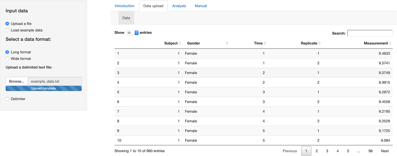
Data upload tab of the tool. The dataset uploaded to the tool as in a long format.
After uploading the data set, we can now move on to the Analysis tab to perform the BV data analysis (Figure 2). There are separate sub-tabs in this section. Outlier detection results can be obtained using Cochran’s test and Reed’s criterion (Figure 2a). The normality assumption can be checked using the Shapiro–Wilk test (Figure 2b). The steady-state condition can be controlled by performing linear regression (Figure 2c). Homogeneity of analytical and within-subject variabilities can be tested using the Bartlett test (Figure 2d). Subset analysis can be performed by comparing 95% confidence intervals of CVI and CVG for males and females (Figure 2e). Nested ANOVA can be carried out to estimate variance components and analytical performance specifications for all-subjects and separately for males and females (Figure 2f). Mean and absolute range plots can be obtained after each outlier detection step (Figure 2g). An analysis report can be generated and downloaded in HTML file format (Figure 2h).
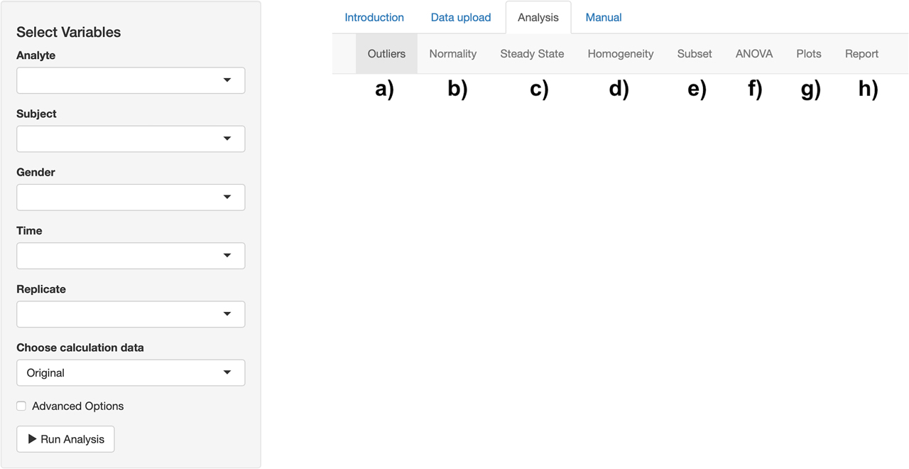
Analysis tab of the tool. a) Outlier results can be obtained. b) The normality assumption can be controlled. c) The steady-state condition can be checked. d) Homogeneity assumptions can be tested. e) Subset analysis can be performed. f) Analysis of variance (ANOVA) components can be estimated. g) Mean and absolute range plots can be created. h) A report can be generated.
BV data analysis
First, outlier detection performed to detect outlying subjects using the Outliers tab. Three replicate measurements were detected as outliers using Cochran’s test (Table 1), and no subjects found as outlying subjects using Cochran’s test and Reed’s criterion. Accordingly, the three outlying replicates were removed from the dataset.
Results of Cochran’s test to detect outliers in the sets of replicates.
| Subject | Time | 1st replication | 2nd replication | Variance | var (mr)/var (sr)* | Critical value |
|---|---|---|---|---|---|---|
| 3 | 1 | 11.9173 | 11.0311 | 0.393 | 0.071 | 0.031 |
| 30 | 5 | 11.815 | 11.0762 | 0.273 | 0.054 | 0.032 |
| 11 | 9 | 11.9003 | 12.4969 | 0.178 | 0.038 | 0.032 |
*var (mr)/var (sr): The ratio of maximum replicate variance to the sum of replicate variances.
Next, we move on to checking the normality assumption using the Normality tab. First, we performed normality tests on sets of results from each individual using the Shapiro–Wilk test and found that all subjects follow normal distributions (all p values > 0.05). Then, we move on to check the normality assumption on mean values of the subjects using the Shapiro–Wilk test, and it is concluded that the data is assumed to be normal on mean values of subjects (p=0.998, Table 2)
Normality test on mean values of subjects.
| Test | Test statistic | p-Value |
|---|---|---|
| Shapiro–Wilk | 0.994 | 0.998 |
Next, the Steady-State tab is used to check whether all subjects were in the steady-state condition during the study period. Linear regression analysis performed on the mean group values over the study period (Table 3), and the steady-state assumption was concluded since 95% confidence interval of the regression coefficient included 0 (95% CI: −0.015 – 0.014).
Linear regression result for mean group values over the study period.
| Variable | Estimate | Std. Error | t value | p-Value | Lower limit | Upper limit |
|---|---|---|---|---|---|---|
| (Intercept) | 10.012 | 0.04 | 252.555 | <0.001 | 9.921 | 10.103 |
| Time | −0.0003 | 0.006 | −0.039 | 0.97 | −0.015 | 0.014 |
The Homogeneity tab is used to test the homogeneity of within-subject and analytical variability (between replicates). The Bartlett test is used to test the homogeneity assumptions, and the test results showed that the homogeneity assumptions are valid (Table 4) for both analytical variability (p=0.940) and within-subject variability (p=0.083).
Homogeneity test results for analytical and within-subject variability.
| Variability | Corrected chi-square | p-Value |
|---|---|---|
| Analytical | 426.244 | 0.94 |
| Within-subject | 60.952 | 0.083 |
The Subset tab is used to determine whether CVI and CVG results should be reported separately for gender groups. Since the 95% confidence intervals of both CVI and CVG overlap between males and females, it is concluded that all-subjects estimates should be reported for CVI and CVG (Table 5).
Gender comparison for between-subject and within-subject variation.
| Gender | Source | CV% | Lower limit | Upper limit |
|---|---|---|---|---|
| Female | Between | 14.033 | 10.874 | 19.728 |
| Male | Between | 14.074 | 10.903 | 19.79 |
| Female | Within | 4.118 | 3.751 | 4.561 |
| Male | Within | 4.324 | 3.941 | 4.786 |
Next, the ANOVA tab is used to display (i) mean of the measurand with its confidence interval, II and the number of samples (Table 6), (ii) ANOVA table (Tables 7), (iii) analytical performance specifications (Tables 8) and (iv) RCV result with lower and upper limits (Table 9). For all subjects; CVA is founded as 0.987% (95% CI: 0.928% – 1.054%), CVI is 4.225% (95% CI: 3.952 – 4.536%), CVG is 13.937% (95% CI: 11.577 – 17.487%), II is 0.303 and RCV is founded as 12.026% (11.292 – 12.866%).
Mean and associated confidence interval of the measurand, index of individuality (II) and the number of samples (n).
| Mean | Lower Limit (95%) | Upper Limit (95%) | II | n |
|---|---|---|---|---|
| 10.022 | 10.009 | 10.034 | 0.303 | 954 |
Analysis of variance results for all subjects.
| Source | Sigma | CV (%) | Lower (95%) | Upper (95%) |
|---|---|---|---|---|
| Between | 1.397 | 13.937 | 11.577 | 17.487 |
| Within | 0.423 | 4.225 | 3.952 | 4.536 |
| Analytical | 0.099 | 0.987 | 0.928 | 1.054 |
| Total | 1.463 | 14.596 | 12.364 | 18.017 |
Analytical performance specifications for all subjects.
| Quality Levels | Imprecision (%) | Bias (%) | Total allowable error (%) |
|---|---|---|---|
| Optimal | <1.056 | <7.36 | <9.103 |
| Desirable | <2.112 | <14.721 | <18.207 |
| Minimal | <3.169 | <22.081 | <27.31 |
Reference change value results.
| RCV (%) | Lower limit (%) | Upper LIMIT (%) |
|---|---|---|
| 12.026 | 11.292 | 12.866 |
The Plot tab can be used to create mean and absolute range plots (Figure 3). These plots are especially useful to inspect outlying subjects and compare subgroups (i.e., genders). Four plots will be displayed in this tab: (i) before outlier detection, (ii) after removing outliers among replicates using Cochran’s test, (iii) after removing outlier subjects using Cochran’s test, and (iv) after removing outlier subjects using Reed’s criterion. Finally, one can download the whole report using the Report tab. The report can be downloaded as an HTML format. The report includes all the results and the tables generated by the tool.
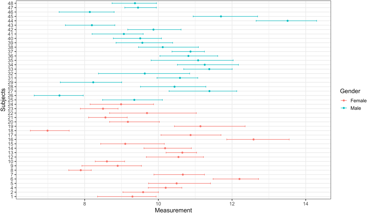
Mean and absolute range plot after removing outliers among replicates using Cochran’s test.
Discussion
The BV data has crucial importance on the correct interpretation of laboratory tests, hence diagnosis and monitoring patients. Statistical analysis of the BV data is as essential as to derive them experimentally. Each step in the statistical analysis procedure should be carried out thoroughly and rigorously. Since even one influential observation might have a significant impact on the variance components of the BV data, this procedure should start with the outlier detection step. This step includes the detection of outliers between replicates, within-subjects, and between subjects, using Cochran’s test and Reed’s criterion. Another important step is checking the normality assumption. Since, the normality assumption is necessary for confidence interval and RCV to be calculated directly [11], this assumption must be controlled before proceeding the analysis. One option in the case of the non-normal distribution is to apply ln-transformation to the BV data. If data follow the normal distribution after the transformation, then the analysis procedure should be continued using the ln-transformed data. CV-ANOVA is another data transformation method, which can be applied independently of the data distribution [11], [16].
Moreover, the estimation of CVI and RCV requires a steady-state condition, where the concentration of measurand does not change systematically during the study period [18]. A data transformation using MoM and lnMoM can be used to create a steady-state-like condition. Furthermore, homogeneity of analytical and within-subject variability should be checked prior to the nested ANOVA analysis to ensure that estimations can be generalized to the whole population [11]. After checking all the necessary assumptions and/or applying appropriate data transformation, the BV data can be analyzed using two-fold nested ANOVA. Here, variance components (CVA, CVI, and CVG) can be estimated, and quality measures (imprecision, bias, and total error) can be obtained. Finally, mean and absolute range plots can be created to inspect the sample results before and after outlier detection visually.
Although the statistical analysis of the BV data has critical importance on obtaining correct results for laboratory tests, there is no easily accessible, freely available, easy-to-use tool to perform such statistical analyses. Here, we presented an online tool for statistical analysis of the BV data based on checklist recommendation by Bartlett et al. (2015) [10], the pipeline by Braga and Panteghini (2016) [3] and the critical appraisal checklist by Aarsand et al. (2018) [11]. The tool is freely available through https://turcosa.shinyapps.io/biovar/, and all source code is available on the Github repository at https://github.com/selcukorkmaz/BioVar. Biovar has been previously used as a descriptor by biological variation: information site for laboratory medicine (http://www.biologicalvariation.com/). Please note that we do not have any connection with this organization.
Research funding: None declared.
Author contributions: All authors have accepted responsibility for the entire content of this manuscript and approved its submission.
Conflict of interest statement: The authors have no conflict of interest.
References
1. Castilla, JA, Alvarez, C, Aguilar, J, Gonzalez-Varea, C, Gonzalvo, MC, et al. Influence of analytical and biological variation on the clinical interpretation of seminal parameters. Hum Reprod 2006;21:847–51. https://doi.org/10.1093/humrep/dei423.Suche in Google Scholar PubMed
2. Aarsand, AK, Roraas, T, Sandberg, S. Biological variation – reliable data is essential. Clin Chem Lab Med 2015;53:153–4. https://doi.org/10.1515/cclm-2014-1141.Suche in Google Scholar PubMed
3. Braga, F, Panteghini, M. Generation of data on within-subject biological variation in laboratory medicine: An update. Crit Rev Clin Lab Sci 2016;53:313–25. https://doi.org/10.3109/10408363.2016.1150252.Suche in Google Scholar PubMed
4. Fraser, C. Biological Variation: from Principles to Practice. Washington (DC): AACC Press; 2001.Suche in Google Scholar
5. Franzini, C. Relevance of analytical and biological variations to quality and interpretation of test results: examples of application to haematology. Ann Ist Super Sanita 1995;31:9–13.Suche in Google Scholar
6. Fraser, CG, Harris, EK. Generation and application of data on biological variation in clinical chemistry. Crit Rev Clin Lab Sci 1989;27:409–37. https://doi.org/10.3109/10408368909106595.Suche in Google Scholar PubMed
7. Fraser, CG, Hyltoft Petersen, P, Libeer, JC, Ricos, C. Proposals for setting generally applicable quality goals solely based on biology. Ann Clin Biochem 1997;34:8–12. https://doi.org/10.1177/000456329703400103.Suche in Google Scholar PubMed
8. Petersen, PH, Fraser, CG. Strategies to set global analytical quality specifications in laboratory medicine: 10 years on from the Stockholm consensus conference. Accredit Qual Assur 2010;15:323–30. https://doi.org/10.1007/s00769-009-0630-8.Suche in Google Scholar
9. Sandberg, S, Fraser, CG, Horvath, AR, Jansen, R, Jones, G, et al. Defining analytical performance specifications: consensus statement from the 1st Strategic Conference of the European Federation of Clinical Chemistry and Laboratory Medicine. Clin Chem Lab Med 2015;53:833–5. https://doi.org/10.1515/cclm-2015-0067.Suche in Google Scholar PubMed
10. Bartlett, WA, Braga, F, Carobene, A, Coskun, A, Prusa, R, et al. A checklist for critical appraisal of studies of biological variation. Clin Chem Lab Med 2015;53:879–85. https://doi.org/10.1515/cclm-2014-1127.Suche in Google Scholar PubMed
11. Aarsand, AK, Roraas, T, Fernandez-Calle, P, Ricos, C, Diaz-Garzon, J, et al. The biological variation data critical appraisal checklist: a standard for evaluating studies on biological variation. Clin Chem 2018;64:501–14. https://doi.org/10.1373/clinchem.2017.281808.Suche in Google Scholar PubMed
12. Kokoska, S, Christopher, N. Statistical tables and formulae. New York, NY: Springer; 198.Suche in Google Scholar
13. Razali, NM, Wah, YB. Power comparisons of shapiro-wilk, kolmogorov-smirnov, lilliefors and anderson-darling tests. J Stat Model Anal 2011;2:21–33.Suche in Google Scholar
14. Sahai, H, Ojeda, MM. Analysis of variance for random models, volume 2: unbalanced data: theory, methods, applications, and data analysis. Berlin: Springer Science & Business Media; 2004.10.1007/978-0-8176-8168-5Suche in Google Scholar
15. Burdick, RK, Borror, CM, Montgomery, DC. Design and analysis of gauge R&R studies: Making decisions with confidence intervals in random and mixed ANOVA models. New Delhi: SIAM; 2005.10.1137/1.9780898718379Suche in Google Scholar
16. Roraas, T, Stove, B, Petersen, PH, Sandberg, S. Biological variation: the effect of different distributions on estimated within-person variation and reference change values. Clin Chem 2016;62:725–36. https://doi.org/10.1373/clinchem.2015.252296.Suche in Google Scholar PubMed
17. Braga, F, Ferraro, S, Ieva, F, Paganoni, A, Panteghini, M. A new robust statistical model for interpretation of differences in serial test results from an individual. Clin Chem Lab Med 2015;53:815–22. https://doi.org/10.1515/cclm-2014-0893.Suche in Google Scholar PubMed
18. Kristoffersen, AH, Petersen, PH, Sandberg, S. A model for calculating the within-subject biological variation and likelihood ratios for analytes with a time-dependent change in concentrations; exemplified with the use of D-dimer in suspected venous thromboembolism in healthy pregnant women. Ann Clin Biochem 2012;49:561–9. https://doi.org/10.1258/acb.2012.011265.Suche in Google Scholar PubMed
19. Aarsand, AK, Diaz-Garzon, J, Fernandez-Calle, P, Guerra, E, Locatelli, M, et al. The EuBIVAS: within- and between-subject biological variation data for electrolytes, lipids, urea, uric acid, total protein, total bilirubin, direct bilirubin, and glucose. Clin Chem 2018;64:1380–93. https://doi.org/10.1373/clinchem.2018.288415.Suche in Google Scholar PubMed
20. Coskun, A, Carobene, A, Kilercik, M, Serteser, M, Sandberg, S, et al. Within-subject and between-subject biological variation estimates of 21 hematological parameters in 30 healthy subjects. Clin Chem Lab Med 2018;56:1309–18. https://doi.org/10.1515/cclm-2017-1155.Suche in Google Scholar PubMed
21. Palomaki, GE, Neveux, LM. Using multiples of the median to normalize serum protein measurements. Clin Chem Lab Med 2001;39:1137–45. https://doi.org/10.1515/cclm.2001.180.Suche in Google Scholar
22. Snedecor, GW, Cochran, WG. Statistical methods, 8th ed. Ames: Iowa State Univ. Press Iowa; 1989.Suche in Google Scholar
23. Carobene, A, Roraas, T, Solvik, UO, Sylte, MS, Sandberg, S, et al. Biological variation estimates obtained from 91 healthy study participants for 9 enzymes in serum. Clin Chem 2017;63:1141–50. https://doi.org/10.1373/clinchem.2016.269811.Suche in Google Scholar PubMed
24. Fraser, CG. Inherent biological variation and reference values. Clin Chem Lab Med 2004;42:758–64. https://doi.org/10.1515/cclm.2004.128.Suche in Google Scholar PubMed
25. Harris, EK. Statistical aspects of reference values in clinical pathology. Prog Clin Pathol 1981;8:45–66.Suche in Google Scholar
26. Fraser, CG. Reference change values. Clin Chem Lab Med 2011;50:807–12. https://doi.org/10.1515/CCLM.2011.733.Suche in Google Scholar PubMed
27. Fokkema, MR, Herrmann, Z, Muskiet, FA, Moecks, J. Reference change values for brain natriuretic peptides revisited. Clin Chem 2006;52:1602–3. https://doi.org/10.1373/clinchem.2006.069369.Suche in Google Scholar PubMed
28. Oosterhuis, WP, Bayat, H, Armbruster, D, Coskun, A, Freeman, KP, et al. The use of error and uncertainty methods in the medical laboratory. Clin Chem Lab Med 2018;56:209–19. https://doi.org/10.1515/cclm-2017-0341.Suche in Google Scholar PubMed
29. Biswas, SS, Bindra, M, Jain, V, Gokhale, P. Evaluation of imprecision, bias and total error of clinical chemistry analysers. Indian J Clin Biochem 2015;30:104–8. https://doi.org/10.1007/s12291-014-0448-y.Suche in Google Scholar PubMed PubMed Central
30. Oosterhuis, WP. Gross overestimation of total allowable error based on biological variation. Clin Chem 2011;57:1334–6. https://doi.org/10.1373/clinchem.2011.165308.Suche in Google Scholar PubMed
31. Roraas, T. Estimating biological variation: methodological and statistical aspects. Bergen: University of Bergen; 2017.Suche in Google Scholar
© 2020 Walter de Gruyter GmbH, Berlin/Boston
Artikel in diesem Heft
- Frontmatter
- Review Article
- Newly developed diagnostic methods for SARS-CoV-2 detection
- Short Communication
- Effect of hemolysis on prealbumin assay
- Research Articles
- BioVar: an online biological variation analysis tool
- High dose ascorbic acid treatment in COVID-19 patients raised some problems in clinical chemistry testing
- Immunoassay biomarkers of first and second trimesters: a comparison between pregnant Syrian refugees and Turkish women
- Association of maternal serum trace elements with newborn screening-thyroid stimulating hormone
- PIK3CA and TP53 MUTATIONS and SALL4, PTEN and PIK3R1 GENE EXPRESSION LEVELS in BREAST CANCER
- Evaluation of E2F3 and survivin expression in peripheral blood as potential diagnostic markers of prostate cancer
- Age, gender and season dependent 25(OH)D levels in children and adults living in Istanbul
- Original Article
- Fractional excretion of magnesium as an early indicator of renal tubular damage in normotensive diabetic nephropathy
- Research Articles
- Diagnostic value of laboratory results in children with acute appendicitis
- Evaluation of thiol disulphide levels in patients with pulmonary embolism
- Relationship between renal tubulointerstitial fibrosis and serum prolidase enzyme activity
- Comparison of test results obtained from lithium heparin gel tubes and serum gel tubes
- MHC Class I related chain A (MICA), Human Leukocyte Antigen (HLA)-DRB1, HLA-DQB1 genotypes in Turkish patients with ulcerative colitis
- An overview of procalcitonin in Crimean-Congo hemorrhagic fever: clinical diagnosis, follow-up, prognosis and survival rates
- Comparison of different equations for estimation of low-density lipoprotein (LDL) – cholesterol
- Case-Report
- A rare case of fructose-1,6-bisphosphatase deficiency: a delayed diagnosis story
- Research Articles
- Atypical cells in sysmex UN automated urine particle analyzer: a case report and pitfalls for future studies
- Investigation of the relationship cellular and physiological degeneration in the mandible with AQP1 and AQP3 membrane proteins
- In vitro assessment of food-derived-glucose bioaccessibility and bioavailability in bicameral cell culture system
- Letter to the Editor
- The weighting factor of exponentially weighted moving average chart