Probabilistic analysis of a thermosetting pultrusion process
-
 ,
,

Abstract
In the present study, the effects of uncertainties in the material properties of the processing composite material and the resin kinetic parameters, as well as process parameters such as pulling speed and inlet temperature, on product quality (exit degree of cure) are investigated for a pultrusion process. A new application for the probabilistic analysis of the pultrusion process is introduced using the response surface method (RSM). The results obtained from the RSM are validated by employing the Monte Carlo simulation (MCS) with Latin hypercube sampling technique. According to the results obtained from both methods, the variations in the activation energy as well as the density of the resin are found to have a relatively stronger influence on the centerline degree of cure at the exit. Moreover, different execution strategies are examined for the MCS to investigate their effects on the accuracy of the random output parameter.
1 Introduction
Pultrusion is a continuous process of manufacturing composite profiles having a constant cross-sectional area. It has been widely used for producing high-strength and lightweight composite structures such as wind turbine blades, ballistic resistance panels, spars of ship hulls, thin-wall panel joiners, door/window frames, and drive shaft of vehicles. A schematic representation of the process can be seen in Figure 1. The reinforcing material (rovings/mats) and the resin matrix are pulled together via a pulling mechanism through the preforming guiders. The wetted reinforcements advance through a heating die and then the cured product is cut into desired final length by a saw mechanism.

Schematic view of a pultrusion process.
Virtual manufacturing, in essence applying a numerical process simulation, is an important step toward designing enduring and better-functioning products in the pultrusion process as well as in other manufacturing processes. There have been several numerical modeling studies specific to the thermo-chemical simulation of the pultrusion process in the literature. Generally, numerical techniques such as the finite difference method and the finite element (FE) method with control volume (CV) technique or the nodal CV (NCV) technique have been used for the simulation of the process [1–7]. According to the results obtained in [1–7], similar temperature and cure degree behaviors have been found. For example, the temperature of the composite initially lags behind the die temperature; however, the composite temperature exceeds the die temperature during curing due to the internal heat generation of the resin. As a means of supporting the numerical thermo-chemical modeling of the pultrusion process, experimental studies of various composite profiles have been carried out in [8–13]. However, the studies [1–14] are limited by the deterministic prescription of the process and its material parameters. The uncertainties in the simulation of composite manufacturing processes, particularly resin transfer molding (RTM), have been studied by several researchers [15–18]. In [15], the effect of variation in the isothermal curing temperature and the resin kinetic parameters on cure time was investigated for the RTM process using the Latin hypercube sampling (LHS) technique. It was concluded that the statistical variation in the curing temperature was found to have a greater impact on the curing time as compared with the change in the resin kinetic parameters. The same sampling technique was used in [16] in order to explore the uncertainties in the preform permeability, the resin viscosity, and the kinetic parameters for the RTM process. The random output variables were determined as the fill time and the maximum cure inside the composite at the end of the non-isothermal filling process during RTM. In [17], the probability of process-induced deformations of a composite part exceeding a specified allowable tolerance was calculated by using the first-order reliability method (FORM) integrated with a deterministic modeling tool, which simulates the various physical phenomena during processing of composite structures. In [18], the sensitivities and the probabilities of the maximum and minimum process temperatures and the cure degree were investigated for the prescribed random input variables by implementing a gradient-based reliability analysis, i.e., FORM. Following the sensitivity analysis, an efficient two-level reliability-based design optimization approach was performed in order to minimize the cure cycle time and associated manufacturing cost for an RTM-kind process. Apart from the composite manufacturing processes, probabilistic analyses of various engineering applications [19–23] have been investigated by using the probabilistic design system (PDS) toolbox of ANSYS [24].
In the present paper, a new application for the probabilistic analysis of the pultrusion process is presented. The effects of the uncertainties in the pultrusion process parameters on the degree of cure at the die exit were investigated. The deterministic analysis was based on a thermo-chemical model of the pultruded AS4/Epon 9420/9470/537 carbon fiber/epoxy composite rod. It was performed for validation purposes using the FE with NCV (FE/NCV) method. For the probabilistic analysis, Monte Carlo simulation (MCS) and the response surface method (RSM), which is the first contribution of its kind in the numerical modeling of pultrusion process, were performed. The LHS technique was used in the MSC and the RSM for generating the sample data. For this purpose, the PDS toolbox of ANSYS was utilized incorporated with a parametric deterministic model developed by the authors using its own scripting language, the ANSYS Parametric Design Language (APDL). This approach gives a better understanding of the effect of the variations or uncertainties inherently present in the process and makes it easier or more practical to predict how large and sensitive the scatter of the output parameters (e.g., exit degree of cure) with respect to scatter in the input design parameters is. In other words, this study provides practical information about the robustness of the process model.
2 Governing equations
The steady-state heat transfer equation in a two-dimensional cylindrical coordinate system for the composite rod can be written as follows [4]:
where T is the temperature, u is the pulling speed, ρ is the density, Cp is the specific heat, and kz and kr are the thermal conductivities in the axial or pulling direction (z) and in the radial direction (r), respectively. Lumped material properties are used for the pultruded composite rod and are assumed to be constant. The internal heat generation q (W/m3) due to the exothermic reaction of the epoxy resin can be expressed as [8]
where Vf is the fiber volume fraction, ρr is the density of the epoxy resin, and Q is the specific heat generation (W/kg) due to the exothermic cure reaction of the resin.
The expression of the degree of cure (α) can be written as the ratio of the amount of heat generated [H(t)] during curing to the total heat of reaction Htr, i.e., α=H(t)/Htr. The rate of the degree of cure, Rr, can be written as an Arrhenius type of equation [8]:
where Ko is the preexponential constant, E is the activation energy, R is the universal gas constant, and n is the order of reaction (kinetic exponent). Ko, E, and n can be obtained by curve-fitting procedure applied to the experimental data evaluated using the differential scanning calorimetry (DSC) tests [8]. As a result, Q [Eq. (2)] can be expressed as follows:
By using the chain rule, the rate of degree of cure (dα/dt) can be expressed as
and from Eq. (5), the steady-state resin kinetics equation is written as
which is used in the thermo-chemical analysis of the pultrusion process.
3 Numerical implementation
The FE/NCV method, which is well documented in the literature [2, 3], was implemented for the steady-state simulation of the pultrusion of the composite rod using the APDL [24]. The internal heat generation [Eq. (2)], together with the resin kinetics equation [Eq. (3)], was coupled with the energy equation [Eq. (1)] in an explicit manner in order to obtain a fast numerical procedure since internal heat generation is highly nonlinear [25]. The degree of cure was subsequently updated explicitly for each NCV using Eq. (6) in its discretized form. The upwind scheme was used for the space discretization of the cure degree (u∂α/∂z) in Eq. (6) in order to obtain a stable solution. The degree of cure, as well as the internal heat generation, was updated explicitly at each node, as mentioned before, according to the calculated steady-state nodal temperature data in ANSYS.
4 Validation case: deterministic analysis
The deterministic thermo-chemical pultrusion simulation of a composite rod taken from the literature [8] was performed as a validation case. The temperature and the cure degree distributions were predicted with a given die wall temperature profile based on the experimental work of Valliappan et al. [8]. The model geometry and the boundary conditions are shown in Figure 2 (left). An axi-symmetrical model was used since the die wall temperature profile [Tw(z) in Figure 2] was assumed to be constant throughout the periphery of the rod. Graphite fiber reinforcement (Hercules AS4-12K) and epoxy resin (SHELL EPON9420/9470/537) system were used for the composite. The thermo-physical properties of the composite are taken from [8] and given in Figure 2 (right). The resin kinetic parameters used in the simulations were the following [8]: Htr=323,700 (J/kg), K0=191,400 (1/s), E=60,500 (J/mol), and n=1.69. The preheating temperature of the composite rod, i.e., Tleft in Figure 2, was taken as the resin bath temperature, 38°C. The initial cure degree of the composite was assumed to be 0. In order to reach the steady state, the convergence limits were defined as the maximum temperature and cure degree difference between the new time step and the old time step, and these were set to 0.001°C and 0.0001, respectively.

Schematic view of the pultrusion model of the composite rod and the corresponding boundary conditions (left). Material properties of the composite rod (right).
The steady-state temperature and cure degree distributions were predicted using the deterministic model with a pulling speed of 30 cm/min. The centerline temperature and degree of cure profiles are depicted in Figure 3. It is seen that the results were found to agree well with the experimental data (for temperature) and the predicted data (for the degree of cure) provided in [8]. This shows that the employed deterministic thermo-chemical model gave converged results with a reliable solution. It is seen in Figure 3 that the centerline temperature of the composite became higher than the die wall temperature in a distance of approximately 380 mm from the die inlet due to the internal heat generation. The peak temperature of the composite was found to be approximately 205°C, and the centerline degree of cure at exit was calculated as 0.844.

Predicted temperature (top) and degree of cure profiles (bottom) at the centerline of the composite rod.
5 Probabilistic analysis
5.1 Probabilistic methods
In the present work, two different probabilistic approaches, in particular, the MCS and the RSM, were implemented using the ANSYS PDS toolbox. The MCS is a sampling-based method, whereas the RSM is a curve fitting or surrogate modeling method that is used to approximate a function in terms of its variables. The details of these methods are explained in the following.
5.1.1 MCS
The MCS is one of the most common sampling techniques used for uncertainty or sensitivity analyses. It is based on random sampling of the input parameters for each simulation loop. The simulation loop or sample mentioned here indicates the iterative execution of a random parameter set. The LHS is selected for the sampling method since no overlap among the sample points is guaranteed, which provides more random (in other words, distributed wide apart) sampling procedure than the direct sampling technique does [20, 24]. Assuming that the deterministic model is correct, the MCS theoretically converges to the correct probabilistic results with an increasing number of samples. This also forces the tails of a distribution to participate in the sampling process, which is often not the case in real-world applications having a limited number of samples [19]. In order to capture the tails in a probability density function, an extremely large number of simulations is required for the MCS. For a given probability of failure (pf), the minimum number of sample points, Nmin, required for the MCS is defined as [26, 27]
where δ is the desired accuracy of the simulation result. It is seen that Nmin is inversely proportional with pf and δ. For instance, for a given probability of 0.9999 (pf=1-0.9999=0.0001) in the tail, around 1 million sample points are needed in order to ensure a 10% accuracy of the estimated result from the MCS. It should be noted that the main focus of the present work was not on the evaluation of very low probabilities (tail probabilities). Despite the high computational cost, the MCS does not use any assumptions or simplifications on the input-output parameters, which makes it easy to use.
The results of the MCS are based on the statistical procedures such as calculation of the mean, the standard deviation, the cumulative density functions, and the correlations. The cumulative distribution function (CDF), here denoted as Fi, of a sampled data is derived from the cumulative binomial distribution function [19, 24, 28]:
where the CDF of the ith sample data out of N, i.e., Fi, is solved numerically in ANSYS for the data sorted in ascending order.
In the present study, a linear correlation was used between the two random variables, e.g., the ith random input variable and the ith output variable. The correlation coefficients are calculated according to the following relation in ANSYS [24]:
where rp is the correlation coefficient between the two random variables x and y, n is the sample size, and x? and y? are the mean of the sample data x and y, respectively.
5.1.2 RSM
A true input-output relationship used in the MCS is replaced with an approximation function in the RSM. The response surfaces are generated with the use of conventional design of experiments (DOE). The accuracy of the results depends on the number of sample points or the DOEs employed in the RSM. There are two main steps in the RSM: The first one is the calculation of the random output parameters by performing sufficient simulation loops based on the sample points, i.e., generation of the response surfaces with the DOEs. The sample points or the DOEs are located in the space of the random input variables where the approximated mathematical function can be obtained most efficiently. The second step is the application of a linear regression analysis to determine the coefficients of the approximation function, which is typically a quadratic polynomial defined as
where
A central composite design (CCD) is one of the commonly used and popular designs for fitting second-order response surfaces (quadratic polynomials). It is widely used in practice due to its efficiency in terms of the number of required function evaluations [29]. The total number of sample points is determined according to the following relation for the CCD design in ANSYS [24]:
which is used to form the corresponding n-dimensional hypercube (response surface) for the number of input variables n. Here, f is the fraction of the factorial points used in ANSYS based on n [24, 29]. In other words, a CCD is composed of two axis points per input variable (i.e., 2n), factorial points at the corner of the hypercube (i.e., 2n-f), and one central point located at the center of the hypercube.
5.2 Description of the probabilistic model
For the probabilistic analysis of the pultrusion process, the pulling speed, fiber volume ratio, inlet temperature, all the characteristic material properties, and the resin kinetic parameters are considered as the random input parameters (RIPs). Table 1 summarizes the total of 14 RIPs and their distributions. Here, GAUSS denotes the Gaussian (normal) distribution with a mean (μ) and a standard deviation (σ), where σ=μ×COV and COV is the coefficient of variation. In general, the statistical characteristics are obtained from extensive data collection and data analysis. In the present study, the mean values of the RIPs were taken from the deterministic analysis and the standard deviations were estimated based on engineering intuition and common available data from the literature [18, 30]. The first three RIPs (process parameters) are more controllable than the material properties, i.e., RIPs between 4 and 10 (Table 1), and hence, the COVs of the first three RIPs selected were lower than the COVs of the RIPs between 4 and 10. The last four RIPs are related with the resin kinetic parameters, which are obtained from a curve-fitting procedure of the DSC data where deviation from the fitting may exist [31, 32] (i.e., 0.01 is used for COV in this work). The centerline degree of cure at the exit (CDOCE) is taken as the random output response since it directly affects the expected mechanical properties of the product as well as the possibility of the defects.
Statistical characteristics of the RIPs for the pultrusion process.
| No. | Parameter | Symbol | Unit | μ | COV | Distribution |
|---|---|---|---|---|---|---|
| 1 | Pulling speed | u | cm/min | 30 | 0.02 | GAUSS |
| 2 | Fiber volume fraction | Vf | – | 0.622 | 0.02 | GAUSS |
| 3 | Inlet temperature | Tleft | °C | 38 | 0.02 | GAUSS |
| 4 | Density of resin | ρr | kg/m3 | 1260 | 0.05 | GAUSS |
| 5 | Density of fiber | ρf | kg/m3 | 1790 | 0.05 | GAUSS |
| 6 | Specific heat of resin | Cpr | J/kg-K | 1255 | 0.05 | GAUSS |
| 7 | Specific heat of fiber | Cpf | J/kg-K | 712 | 0.05 | GAUSS |
| 8 | Thermal conductivity of resin | kr | W/m-K | 0.2 | 0.05 | GAUSS |
| 9 | Thermal conductivity of fiber in r-axis | (kr)f | W/m-K | 11.6 | 0.05 | GAUSS |
| 10 | Thermal conductivity of fiber in z-axis | (kz)f | W/m-K | 66.0 | 0.05 | GAUSS |
| 11 | Total heat of reaction | Htr | J/kg | 323,700 | 0.01 | GAUSS |
| 12 | Pre-exponential constant | Ko | 1/s | 191,400 | 0.01 | GAUSS |
| 13 | Activation energy | E | J/mol | 60,500 | 0.01 | GAUSS |
| 14 | Order of reaction | n | – | 1.69 | 0.01 | GAUSS |
Two different probabilistic case studies (case 1 and case 2), each having two subcases, were performed, and the summary of these case studies is given in Table 2. The total number of DOEs used in the RSM was calculated from the relation given in Eq. (11). In Eq. (11), f was specified as 3 and 6 for case 1 (n=10) and case 2 (n=14), respectively, as reported in ANSYS [24]. As a result, 149 sample points for case 1 and 285 sample points for case 2 were obtained from the expression presented in Eq. (11) for the CCD design in the RSM. The details of the case studies are explained in the following.
Case 1: Only the first 10 RIPs were used for the MCS (case 1.1) and the RSM (case 1.2) in order to determine the effect of the variation in the process parameters and the material properties on the variation of the output parameter.
Case 1.1: An MCS having a total of 1000 simulations (samples) was performed based on three different MCS options to investigate their effects on the accuracy of the output parameter:
Case 1.1a (full MCS): 1000 simulations were divided into one repetition (cycle) such that all 1000 samples were initially selected at once by using the LHS technique.
Case 1.1b (incremental MCS): 1000 simulations were divided into 10 repetitions such that the 1000 simulations were performed in 100 simulations with 10 repetitions. This added more randomness to the LHS procedure.
Case 1.1c (adaptive MCS): 1000 simulations were divided into one repetition with the adaptive stopping criterion option where the MCS was terminated before the total simulations were done if the convergence criterion was met. This states that the change in the mean and standard deviation of the random output parameter should be lower than or equal to 0.001 in the consecutive MCS iterations.
Case 1.2: The RSM was utilized where 149 DOEs (sample points) were required for generating the response surface (quadratic polynomial) for 10 RIPs by using the CCD design. In addition to the DOEs, 10,000 Monte Carlo runs were performed for exploiting the response surface, which took only about a couple of seconds.
Case 2: All the RIPs in Table 1 (total of 14) were used for the MCS (case 2.1) and the RSM (case 2.2) in order to investigate the effect of the variation in the resin kinetic parameters as well as the process parameters and material properties on the variation in the output parameter.
Case 2.1: An MCS with LHS having a total of 1000 samples was performed according to the results of case 1.1 based on the best MCS option found so far.
Case 2.2: RSM was utilized where 285 DOEs plus 10,000 MCS runs were performed for 14 RIPs using the CCD.
Summary of the probabilistic case studies.
| Analysis type | Number of RIPs | Number of MCS loops | Number of DOEs | ||
|---|---|---|---|---|---|
| Case 1 | Case 1.1 | MCS | 10 | 1000 | – |
| Case 1.2 | RSM | 10 | 10,000 | 149 | |
| Case 2 | Case 2.1 | MCS | 14 | 1000 | – |
| Case 2.2 | RSM | 14 | 10,000 | 285 |
6 Results and discussion
6.1 Case 1
In order to obtain statistical significance (to have a more general conclusion), a total of 10 separate MCS runs, i.e., 10×1000 simulations, were performed for case 1.1 (i.e., for each option: case 1.1a, full MCS; case 1.1b, incremental MCS; and case 1.1c, adaptive MCS). The 10,000 sequential runs required about 80 h using a Intel 2.3 GHz quad core processor. The results and discussion of case 1 are explained in the following:
Table 3 shows the mean values of the linear correlation coefficients between the RIPs and the corresponding output parameter (the CDOCE) for 10 separate runs. It is seen that the mean values of the correlation coefficients were very close to each other for the three options of case 1.1, which indicates that the MCS converged for 1000 samples.
However, the standard deviations of the 10 runs for these three options differed, as seen in Table 4 as a percentage of the mean values given in Table 3. The incremental MCS option had the lowest magnitude of standard deviation for the 6 RIPs out of 10, i.e., u, Vf, ρf, ρr, Cpf, and Cpr. This shows that the incremental MCS is more accurate than the full MCS and the adaptive MCS since the LHS produced more random and diverse solutions in the incremental MCS.
The overall mean of the first three rows in Table 3 (correlation coefficients) is given as mean in the last row of the table. The same correlation coefficients, i.e., mean, are seen as a bar plot in Figure 4 (right). As seen from this plot, ρr had the highest (and only) positive correlation coefficient (rp=0.587), and the rest had a lower negative correlation with the CDOCE. Here, a positive correlation indicates that the input parameter is directly proportional with the output parameter and vice versa. The corresponding sensitivities are also given in the pie chart in Figure 4 (right) based on the correlation coefficients. The percentage values indicate how sensitive the CDOCE is with respect to the statistical variations in the RIPs.
The CDF of the CDOCE is shown in Figure 4 (left) for 10 runs of each MCS option described in case 1.1. It is seen that the CDFs for all runs (3×10) were found to be close to each other.
The sampling range of the CDOCE was found to be approximately between 0.823 and 0.869 (i.e., 0.844 in average with 0.7% standard deviation), as seen from the horizontal axis of Figure 4 (left). The value of the CDF at each point indicates the probability of the CDOCE being less than a certain level. For instance, the probability of the CDOCE being less than 0.835 is approximately 5%, whereas the probability of the CDOCE being greater than 0.852 is around 100–90=10%.
In case 1.2, 10,000 MCSs exploiting the response surface that require 149 DOEs were performed. The CDFs of case 1.1 (1000 MCSs) and case 1.2 (RSM—10,000 MCSs) are depicted in Figure 5 by using the Gauss plot in order to better visualize the tails of the distribution. Of 10 results taken from the incremental MCS option, one is depicted in Figure 5 for case 1.1 (1000 MCS). It is seen that the MCS results were found to agree with the RSM results in general; however, at the tails of the CDFs for the MCS, results diverged from the RSM results because of the limited sample size, as aforementioned.

CDFs of each option in case 1 for 10 separate runs (left). The linear correlation coefficients (mean values of the three options in case 1.1 for 10 runs) between the RIPs and the CDOCE are shown in the bar plot, and the corresponding sensitivities are shown in the pie chart (right).
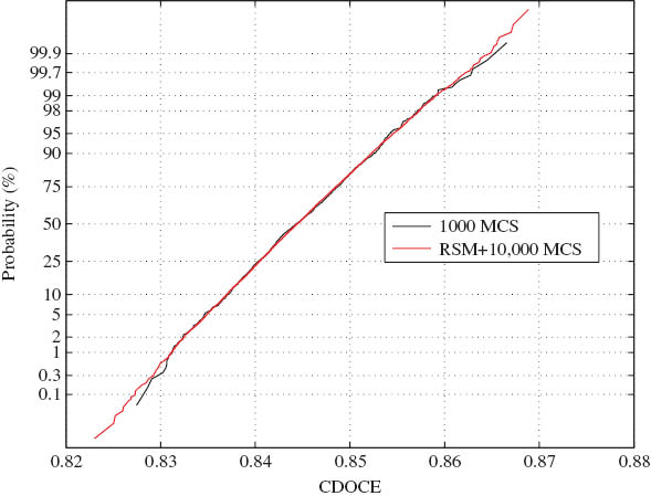
CDFs of case 1.1 (1,000 MCS with LHS) and case 1.2 (RSM+10,000 MCS) in the form of a Gauss plot.
Mean values of the correlation coefficients between the RIPs and the random output parameter (CDOCE) for 10 runs based on each MCS options in case 1.1.
| u | Vf | (kz)f | (kr)f | kr | ρf | ρr | Cpf | Cpr | Tleft | |
|---|---|---|---|---|---|---|---|---|---|---|
| Case 1.1a | -0.470 | -0.491 | -0.018 | -0.018 | -0.283 | -0.284 | 0.590 | -0.102 | -0.086 | -0.013 |
| Case 1.1b | -0.470 | -0.502 | -0.009 | -0.020 | -0.273 | -0.295 | 0.594 | -0.108 | -0.080 | 0.002 |
| Case 1.1c | -0.468 | -0.496 | -0.008 | -0.011 | -0.260 | -0.307 | 0.578 | -0.105 | -0.087 | -0.022 |
| Mean | -0.470 | -0.496 | -0.012 | -0.016 | -0.272 | -0.296 | 0.587 | -0.105 | -0.085 | -0.011 |
Case 1.1a, full MCS; case 1.1b, incremental MCS; and case 1.1c, adaptive MCS.
Standard deviations of the correlation coefficients between the RIPs and the random output parameter (CDOCE) for 10 runs based on each MCS options of case 1.1.
| u | Vf | (kz)f | (kr)f | kr | ρf | ρr | Cpf | Cpr | Tleft | |
|---|---|---|---|---|---|---|---|---|---|---|
| Case 1.1a | -4.31 | -4.46 | -151.81 | -234.90 | -11.93 | -10.34 | 3.30 | -28.24 | -39.25 | -118.55 |
| Case 1.1b | -3.17 | -1.49 | -301.09 | -214.99 | -11.74 | -3.48 | 1.83 | -25.45 | -31.83 | 1525.34 |
| Case 1.1c | -6.28 | -4.01 | -479.34 | -206.85 | -9.18 | -6.79 | 3.19 | -37.10 | -51.67 | -264.34 |
The standard deviation values are given in percentage (%) of the mean values given in Table 3.
6.2 Case 2
The MCS with the LHS was performed for 1000 samples in case 2.1 based on the incremental MCS option defined in case 1. On the other hand, in case 2.2, 10,000 Monte Carlo runs exploiting the response surfaces that require 285 DOEs were performed. The results and discussion of case 2 are explained in the following:
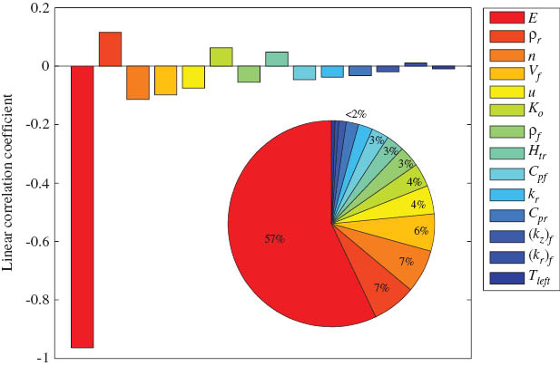
The correlation coefficients between the RIPs (total of 14) and the CDOCE are given as a bar plot in Figure 6 for case 2.1. It is seen that the E (activation energy) had the highest correlation coefficient (negative) and the magnitude was close to 1 (rp=0.964), indicating that E was strongly correlated (i.e., inversely proportional) with the CDOCE. This agrees with a similar observation obtained in [18] for the RTM process, where the effect of the variation in E on the maximum and minimum cure degree was found to be significant. The corresponding sensitivities are depicted as a pie chart in Figure 6. It is seen that the parameter E covered almost 57% of all the sensitivity distribution and the rest of the RIPs were sorted in a similar manner as in case 1.
The five most sensitive linear correlation coefficients among the RIPs and the CDOCE in case 2 are given in Table 5. It is seen that the linear correlation coefficients were almost the same for the two cases, i.e., case 2.1 and case 2.2.
The Gauss plots of the CDFs in case 2, together with those in case 1, are shown in Figure 7. It is seen that the overall MCS results agreed with the RSM results. The sampling range of the CDOCE was found to be approximately between 0.725 and 0.915 in case 2, which was wider than the range found in case 1. This shows that the variation in the resin kinetic parameters (especially in E) had a more significant effect on the CDOCE as compared with the variation in the process parameters and the material properties.
The mean and the standard deviation of the CDOCE were calculated approximately as 0.843 and 3.3% in case 2.
Linear correlation coefficients between the RIPs and the CDOCE in the bar plot and corresponding sensitivities in the pie chart for case 2.1.

Gauss plots of the CDFs calculated in case 1 and case 2.
Five most sensitive linear correlation coefficients between the RIPs and the CDOCE in case 2.
| E | ρr | n | Vf | u | |
|---|---|---|---|---|---|
| Case 2.1 (MCS) | -0.964 | 0.107 | -0.114 | -0.087 | -0.065 |
| Case 2.2 (RSM) | -0.962 | 0.130 | -0.111 | -0.097 | -0.105 |
7 Conclusions
In the present work, a deterministic thermo-chemical simulation for the pultrusion of a composite rod was carried out and the results were found to agree well with the data from the literature [8]. After validating the deterministic model, a probabilistic analysis of the pultrusion process was performed in which two different probabilistic case studies were investigated. For this purpose, the MCS and the RSM, which is the first contribution of its kind for the probabilistic modeling of pultrusion, were employed. The LHS technique was utilized for the sampling procedure in the ANSYS PDS toolbox. The outcomes of this study are summarized as follows:
The effects of the MCS options in ANSYS were investigated in case 1.1, and it was found that the most accurate statistical results were obtained by dividing the total number of simulations (samples) into repetitions; i.e., a total of 1000 simulations were performed in 100 simulations with 10 repetitions using the LHS (here denoted as the “incremental MCS”).
In both cases, i.e., in case 1 and case 2, it was concluded that the overall MCS results (total of 1000 samples) were almost converged to the results obtained from the RSM. Note that the tails of the probability density function was not considered in this work.
Variation in the density of the resin was found to have the most significant influence (positive correlation) on the CDOCE out of 10 RIPs in case 1.
On the other hand, 14 RIPs were considered in case 2, and it was found out that variation in the activation energy (E) of the resin has a very strong correlation (negative) with the CDOCE. This shows that variation in the resin kinetic parameters (especially in E) has a more significant effect on the CDOCE as compared with variation in the process parameters and the material properties. Hence, it is very important to characterize the resin system correctly while using E together with the resin density.
Acknowledgments
This work is a part of the DeepWind project, which has been granted by the European Commission (EC) under the FP7 program platform Future Emerging Technology.
References
[1] Baran I, Tutum CC, Hattel JH. Key Eng. Mater. 2013, 554–557, 2127–2137.10.4028/www.scientific.net/KEM.554-557.2127Search in Google Scholar
[2] Joshi SC, Lam YC. J. Mater. Process. Technol. 2006, 174, 178–182.10.1016/j.jmatprotec.2006.01.003Search in Google Scholar
[3] Liu XL, Crouch IG, Lam YC. Compos. Sci. Technol. 2000, 60, 857–864.10.1016/S0266-3538(99)00189-XSearch in Google Scholar
[4] Baran I, Tutum CC, Hattel JH. Compos. Part B: Eng. 2013, 45, 995–1000.10.1016/j.compositesb.2012.09.049Search in Google Scholar
[5] Baran I, Tutum CC, Nielsen MW, Hattel JH. Compos. Part B: Eng. 2013, 51, 148–161.10.1016/j.compositesb.2013.03.031Search in Google Scholar
[6] Carlone P, Palazzo GS, Pasquino R. Math Comput. Model 2006, 44, 701–709.10.1016/j.mcm.2006.02.006Search in Google Scholar
[7] Baran I, Tutum CC, Hattel JH. Appl. Compos. Mater. 2012, 20, 449–463.10.1007/s10443-012-9278-3Search in Google Scholar
[8] Valliappan M, Roux JA, Vaughan JG, Arafat ES. Compos. Part B: Eng. 1996, 27, 1–9.10.1016/1359-8368(95)00001-1Search in Google Scholar
[9] Chachad YR, Roux JA, Vaughan JG, Arafat E. J. Reinf. Plast. Compos. 1995, 14, 495–512.10.1177/073168449501400506Search in Google Scholar
[10] Ding Z, Li S, Lee LJ. Polym. Compos. 2002, 23, 957–969.10.1002/pc.10493Search in Google Scholar
[11] Chachad YR, Roux JA, Vaughan JG. Eng. Plast. 1996, 9, 91–108.Search in Google Scholar
[12] Roux JA, Vaughan JG, Shanku R, Arafat ES, Bruce JL, Johnson VR. J. Reinf. Plast. Compos. 1998, 17, 1557–1578.10.1177/073168449801701705Search in Google Scholar
[13] Liu XL, Hillier W. Compos. Struct. 1999, 47, 581–588.10.1016/S0263-8223(00)00029-5Search in Google Scholar
[14] Carlone P, Baran I, Hattel JH, Palazzo GS. Adv. Mech. Eng. 2013, 301875.10.1155/2013/301875Search in Google Scholar
[15] Padmanabhan SK, Pitchumani R. Polym. Compos. 1999, 20, 72–85.10.1002/pc.10336Search in Google Scholar
[16] Padmanabhan SK, Pitchumani R. Int. J. Heat Mass Transfer 1999, 42, 3057–3070.10.1016/S0017-9310(98)00377-9Search in Google Scholar
[17] Li H, Foschi R, Vaziri R, Fernlund G, Poursartip A. J. Compos. Mater. 2002, 36, 1967–1991.10.1177/0021998302036016241Search in Google Scholar
[18] Bebamzadeh A, Haukaas T, Vaziri R, Poursartip A, Fernlund G. J. Compos. Mater. 2010, 44, 1821–1840.10.1177/0021998310366062Search in Google Scholar
[19] Reh S, Beley JD, Mukherjee S, Khor EH. Struct. Saf. 2006, 28, 17–43.10.1016/j.strusafe.2005.03.010Search in Google Scholar
[20] Cai B, Liu Y, Liu Z, Tian X, Ji R. Zhang Y. Eng. Fail. Anal. 2012, 19, 97–108.10.1016/j.engfailanal.2011.09.009Search in Google Scholar
[21] Nakamura T, Fujii K. Aerosp. Sci. Technol. 2006, 10, 346–354.10.1016/j.ast.2006.02.002Search in Google Scholar
[22] Zhang Y, Qi Z, Lang X, Zhao M. Appl. Mech. Mater. 2012, 130–134, 887–890.10.4028/www.scientific.net/AMM.130-134.887Search in Google Scholar
[23] Liu PF, Zheng JY. J. Loss Prevent. Proc. 2010, 23, 421–427.10.1016/j.jlp.2010.02.002Search in Google Scholar
[24] User’s Manual of ANSYS 13.0, Canonsburg, PA: ANSYS Inc., 2010.Search in Google Scholar
[25] Baran I, Hattel JH, Tutum CC. Appl. Compos. Mater. 2013, 20, 1247–1263.10.1007/s10443-013-9331-xSearch in Google Scholar
[26] Elishakoff I, Li Y, Starnes JH. Non-Classical Problems in the Theory of Elastic Stability, New York, USA: Cambridge University Press, 2001.10.1017/CBO9780511529658Search in Google Scholar
[27] Handscomb DC, Hammersley JM. Monte Carlo Methods, London, UK: Methuen, 1964.10.1007/978-94-009-5819-7Search in Google Scholar
[28] Kececioglu D. Reliability Engineering Handbook, vol. 2, Upper Saddle River, NJ: Prentice-Hall, 1991.Search in Google Scholar
[29] Montgomery DC, Runger GC. Applied Statistics and Probability for Engineers, 3rd ed., New York, USA: John Wiley&Sons, Inc., 2003.Search in Google Scholar
[30] Baran I, Tutum CC, Hattel JH. Appl. Compos. Mater. 2012, 20, 639–653.10.1007/s10443-012-9293-4Search in Google Scholar
[31] He Y. Thermochim. Acta 2001, 367–368, 101–106.10.1016/S0040-6031(00)00654-7Search in Google Scholar
[32] Wang J, Fang X, Wu M, He X, Liu W, Shen X. Eur. Polym. J. 2011, 47, 2158–2168.10.1016/j.eurpolymj.2011.08.005Search in Google Scholar
©2016 by De Gruyter
This article is distributed under the terms of the Creative Commons Attribution Non-Commercial License, which permits unrestricted non-commercial use, distribution, and reproduction in any medium, provided the original work is properly cited.
Articles in the same Issue
- Frontmatter
- Review
- The behaviour of aluminium matrix composites under thermal stresses
- Original articles
- Preparation and characterization of graphite/resin composite bipolar plates for polymer electrolyte membrane fuel cells
- Synergistic effect of carbon nanotubes in combination with magnesium hydroxide on the flame retardant poly(ethylene-co-vinyl acetate)
- Preparation and characterization of nano biphasic calcium phosphate/poly-L-lactide composite scaffold
- Durability study of ramie fiber fabric reinforced phenolic plates under humidity conditions
- Synthesis and molecular dynamics simulation of hyperbranched poly(amine-ester)/neodymium nanocomposites
- Investigation on wear properties of AZ31-MWCNT nanocomposites fabricated through mechanical alloying and powder metallurgy
- Probabilistic analysis of a thermosetting pultrusion process
- Analysis of shrinkage and creep behaviors in polymer-coated lightweight concretes
- Investigation of optimum cutting parameters and tool radius in turning glass-fiber-reinforced composite material
- Buckling and vibration analyses of composite laminates with weak interfaces by a coupled meshfree and finite element method
- Free vibration and postbuckling of laminated composite Timoshenko beams