Free vibration and postbuckling of laminated composite Timoshenko beams
-
 ,
,

Abstract
A numerical solution method was developed to investigate the postbuckling behavior and vibrations around the buckled configurations of symmetrically and unsymmetrically laminated composite Timoshenko beams subject to different boundary conditions. The Hamilton principle was employed to derive the governing equations and corresponding boundary conditions which are then discretized by introducing a set of matrix differential operators. The pseudo-arc-length continuation method was used to solve the postbuckling problem. To study the free vibration that takes place around the buckled configurations, the corresponding eigenvalue problem was solved by means of the postbuckling configuration modes obtained in the previous step. The static bifurcation diagrams for composite beams with different lay-up laminates are given, and it is shown that the lay-up configuration considerably affects the magnitude of critical buckling load and postbuckling behavior. The study of the vibrations of composite beams with different laminations around the buckled configurations indicates that the natural frequency in the prebuckling domain increases as the stiffness of a beam increases, while there is no specific relation between the lay-up lamination and natural frequency in the postbuckling domain which necessitates conducting an accurate analysis in this area.
1 Introduction
Nowadays, laminated composite structures have several applications in different engineering fields such as aeronautical, automobile, and aerospace industries. Among different laminated composite structures, composite beams are extensively used in civil and mechanical engineering structures because of their high strength-to-weight and high stiffness-to-weight ratios over the conventional isotropic beams. Accordingly, the research topic on buckling [1–10] and vibration [11–20] of these structures has attracted much attention in the literature.
Aydogdu [3] studied the thermal buckling of cross-ply laminated composite beams under different types of boundary conditions based on a three-degree-of-freedom shear deformable beam theory. He solved the problem using the Ritz method with the polynomial series and showed that some cross-ply beams buckle upon cooling rather than heating and some of them do not buckle regardless of whether they are heated or cooled. Gupta et al. [5] applied the Rayleigh-Ritz technique to obtain closed-form expressions for the postbuckling of composite beams subject to different boundary conditions with axially immovable ends. Baghani et al. [6] used the variational iteration method to investigate the postbuckling of unsymmetrically laminated composite beams on a nonlinear elastic foundation. Their study revealed that the beam response can be controlled by a suitable lay-up configuration of the laminate. Emam [7] investigated the significance of the shear deformation on the static postbuckling response of composite beams. It was indicated that classical and first-order theories tend to underestimate the amplitude of buckling load. Vo and Thai [9] employed a refined shear deformation theory to analyze the buckling behavior of composite beams. They developed a two-node C1 beam element of five degrees of freedom per node to carry out the analysis. Dong and co-workers [13] studied the free vibration of a stepped laminated composite Timoshenko beam considering the effect of shear deformation and rotary inertia. Based on the Timoshenko beam theory (TBT), Çalım [14] investigated the free and forced vibrations of non-uniform composite beams in the Laplace domain. The problem was numerically solved by the complementary function method, and it was concluded that the non-uniformity parameters and angle of fiber orientation have significant effect on the dynamic response of non-uniform composite beams. Ghayesh et al. [16] analytically studied the vibrations and stability of an axially traveling laminated composite beam based on the method of multiple scales. Kim and Wang [17] applied a finite element-based formal asymptotic expansion method to study the free vibration of composite beams. Ghayesh [19] conducted a parametric study on the dynamic response of an axially traveling laminated composite beam with special consideration to natural frequencies, complex mode functions, and critical speeds of the system. Recently, Jafari-Talookolaei and his associates [20] studied the free vibration of laminated composite beams using the TBT and the method of Lagrange multipliers.
Also, it is of great technical importance to study the vibrations of buckled beams. There are several papers in the literature in which the vibration of beams around the buckled configurations has been studied (e.g., [21–23]). In 2008, Nayfeh and Emam [21] published a paper on the postbuckling and vibrations of isotropic Euler-Bernoulli beams. They conducted a closed-form solution for the postbuckling configurations of beams under different boundary conditions in terms of the applied axial load. The vibration around buckled configurations was also analyzed in that work. Later, Emam and Nayfeh [22] extended their previous work on the isotropic Euler-Bernoulli beams to the composite Euler-Bernoulli beams.
Unlike the Euler-Bernoulli beam theory (EBT), the TBT considers the effects of transverse shear deformation and rotary inertia. The difference between the results of these theories becomes more prominent for short beams, which might be encountered in some engineering applications. Motivated by this, the aim of the present work is to extend the study of Emam and Nayfeh [22] based on the EBT to the TBT. By developing a new numerical solution approach, the postbuckling and vibrations around the buckled configurations of laminated composite Timoshenko beams are studied in this paper. It should be noted that the vibration problem around the first three buckled configurations is solved here, while the solution given in [22] is only for vibration around the first buckled configuration. The effect of in-plane inertia is taken into account, and the analysis is carried out for beams under simply supported-simply supported (SS), clamped-clamped (CC), and simply supported-clamped (SC) boundary conditions. Also, the solution is presented for composite beams with both symmetric and unsymmetric lay-up configurations of the laminate. First, the governing equations and boundary conditions are derived via the Hamilton principle. Based on the generalized differential quadrature (GDQ) technique, differential matrix operators are introduced so as to discretize the governing equations and boundary conditions. The pseudo-arc-length continuation method is employed to determine the postbuckling configurations. To study the vibrations around the buckled equilibrium positions, the corresponding eigenvalue problem is numerically solved using the postbuckling configuration modes which are obtained by the pseudo-arc-length method.
2 Timoshenko beam formulation
The stored strain energy in a continuum constructed by a linear elastic material occupying region Ω undergoing infinitesimal deformations is expressed as
where εij and σij are the strain and stress tensors given by
in which ui denotes the components of the displacement vector u and δ is the Kronecker delta. λ and u can be obtained by [24]
Consider a beam of length L, cross-section A, and thickness h subjected to an axial compressive load N0. According to the TBT, the displacement components can be written as
where U(t, x), W(t, x), and ψ(t, x) are the axial displacement of the center of sections, lateral deflection of the beam, and the rotation angle of the cross-section with respect to the vertical direction, respectively. The von Karman nonlinear strain-displacement relations are given by
The main components of the symmetric section of the stress tensor can be written in the following forms:
where ks is a correction factor which shows the non-uniformity of shear strain over the beam cross-section. The strain energy with respect to the initial configuration, Πs, the kinetic energy of beam, Πτ, and work done by the axial force, Πw, can be expressed as
where the normal resultant force Nx, shear force Qx, and bending moment Mx in a section are defined as
For a composite beam, the stiffnesses are defined as
where n denotes the number of layers, b is the width of the beam, and Zk and Zk-1 are the distances from the beam reference surface to the outer and inner surfaces of the kth layer, respectively.
in which m=cosθ and n=sinθ (θ is the angular orientation of the fibers), and Q is the stiffness matrix. Also, the inertia terms can be given by
where ρk is the density of the kth layer.
By applying the Hamilton principle, the governing equilibrium equations and corresponding boundary conditions of a composite beam are obtained as
By introducing the non-dimensional parameters
the governing equations can be rewritten as
where
and boundary conditions are
for CC beams,
for SS beams, and
for SC beams.
3 Differential matrix operators
Consider the column vector F as
in which f(xi) shows the value of f(x) at each grid point xi and N symbolizes the number of grid points. Similarly, the values of the rth derivative of f(x) at each point can be defined through the following column vector:
Based on the GDQ method [25], one can arrive at
where the differential matrix operator
where i, j=1, 2, …, N and δ denotes the Kronecker delta. Also, Pk is expressed as
Using the shifted Chebyshev-Gauss-Lobatto grid points, the mesh generation in the x direction can be given by
4 Pseudo-arc-length method
The pseudo-arc-length continuation [26] is a technique to approximate the solution set of a system of nonlinear equations such as F(V, p)=0, for different values of the system parameter p, in which F: ℝN+1→ ℝN:(V, p)→F(V, p) and V∈ ℝN.
First, it is necessary to select an initial point on the solution path. Each point in the algorithm consists of two distinct stages known as the prediction stage and the correction stage. In the prediction stage, the next point on the path,
In the correction stage, in order to improve the predicted point
The main problem in solving this augmented system is to satisfy the constraint F(Xi+1)=0. Furthermore, it is required that Xi+1 be on the hyperplane which passes through
and after that normalizing
5 Buckling problem
For the buckling problem, in order to obtain the static configuration of the beam, the inertia terms
with N entries equal to the number of grid points. In Eq. (30),
where ∘ denotes the Hadamard product (if A=[Aij]N×M and B=[Bij]N×M, then the Hadamard product of these matrices takes the form
for CC beams,
for SS beams, and
for SC beams. Note that
which is solved by the pseudo-arc-length continuation method. It should be noted that with the aim of satisfying the boundary conditions, during the nonlinear solution procedure, the residual of equations of boundaries is inserted into the residual vector of domain that is obtained from the set of nonlinear equations of (35). To accomplish this aim, the elements of the residual vector of domain equivalent to the grid points at the boundaries are replaced with the residual values of boundaries which are obtained from one of the equations of (32), (33), or (34).
6 Vibration around the buckled configurations
To study the free vibration of a buckled beam, a small disturbance around the buckled configurations is considered. Accordingly, the field variables of governing equations can be split into two static and dynamic parts as
where subscript s and d denote the static configuration of a beam in the buckling problem and small dynamic disturbance around the buckled configuration, respectively. By substituting Eq. (36) into (16), one can arrive at
and the boundary conditions become
for CC beams,
for SS beams, and
for SC beams. In order to investigate the linear vibration around the buckled configurations of beams, the nonlinear terms are ignored and the following relations are substituted into Eqs. (37):
The final form of governing equations for the vibration is obtained as
where ω is the natural frequency and
and the boundary conditions can be written as
for CC beams,
for SS beams, and
for SC beams. Note that
where
in which 〈〉 denotes diag(). After imposing the end conditions by substituting all the boundary conditions into the discretized governing equations, Eq. (47) can be expressed as an eigenvalue problem. Rearranging the quadrature analogs of field equations and associated boundary conditions within the framework of a generalized eigenvalue problem yields
in which the superscripts b and d refer to the boundary and domain grid points, respectively. The displacement vectors Xd and Xb are defined by
Using the condensation technique, Eq. (49) is given in the following standard form:
from which the natural frequencies and corresponding vibration mode shapes of the beam in different buckled configurations can be extracted. It must be noted that rather than sorting the eigenvalues according to their values, they are sorted in accordance with the vibration modes for any given value of the applied axial load.
7 Results and discussion
In this section, graphite/epoxy laminated composite beams which have six layers of uniform thickness are considered for generating the numerical results [22]. The material properties are
The dimensions (L×b×h) of the beams are assumed to be 250 mm×10 mm×1 mm for Table 1, and 250 mm× 10 mm×10 mm for Table 2 and all figures. Also, the shear correction factor is considered equal to 5/6.
First five critical buckling loads (N) for different laminates of CC, SC, and SS beams (L/h=250).
| Laminate | Unidirectional | (0°, 90°, 90°)s | (90°, 90°, 0°)s | Cross-ply | ||||
|---|---|---|---|---|---|---|---|---|
| TBT (Present) | EBT [22] | TBT (Present) | EBT [22] | TBT (Present) | EBT [22] | TBT (Present) | EBT [22] | |
| CC beams | ||||||||
| Pcr1 | 81.7995 | 81.9823 | 59.4909 | 59.5876 | 9.197 | 9.19926 | 6.3988 | 6.39991 |
| Pcr2 | 166.8764 | 167.715 | 121.4574 | 121.901 | 18.8088 | 18.8194 | 13.0875 | 13.0926 |
| Pcr3 | 325.0225 | 327.929 | 236.8108 | 238.35 | 36.7602 | 36.797 | 25.5818 | 25.5996 |
| Pcr4 | 488.8994 | 495.731 | 356.6914 | 360.314 | 55.539 | 55.6261 | 38.6568 | 38.699 |
| Pcr5 | 723.2865 | 737.841 | 528.5573 | 536.288 | 82.6068 | 82.7934 | 57.5089 | 57.5992 |
| SC beams | ||||||||
| Pcr1 | 41.8762 | 41.9288 | 30.4475 | 30.4753 | 4.7042 | 4.70484 | 3.2728 | 3.27315 |
| Pcr2 | 123.5013 | 123.933 | 89.8504 | 90.0785 | 13.9011 | 13.9065 | 9.6721 | 9.67475 |
| Pcr3 | 245.2327 | 246.912 | 178.5752 | 179.464 | 27.6848 | 27.7061 | 19.2648 | 19.2751 |
| Pcr4 | 406.2802 | 410.879 | 296.2038 | 298.641 | 46.0463 | 46.1048 | 32.0467 | 32.0751 |
| Pcr5 | 605.596 | 615.836 | 442.1761 | 447.61 | 68.9723 | 69.1031 | 48.0116 | 48.0749 |
| SS beams | ||||||||
| Pcr1 | 20.4841 | 20.4956 | 14.8908 | 14.8969 | 2.2997 | 2.29982 | 1.5999 | 1.59998 |
| Pcr2 | 81.7995 | 81.9823 | 59.4909 | 59.5876 | 9.197 | 9.19926 | 6.3988 | 6.39991 |
| Pcr3 | 183.537 | 184.46 | 133.5835 | 134.072 | 20.6867 | 20.6983 | 14.3942 | 14.3998 |
| Pcr4 | 325.0226 | 327.929 | 236.8108 | 238.35 | 36.7602 | 36.797 | 25.5818 | 25.5996 |
| Pcr5 | 505.3281 | 512.39 | 368.6776 | 372.422 | 57.4054 | 57.4954 | 39.9559 | 39.9995 |
First five critical buckling loads (kN) for different laminates of CC, SC, and SS beams (L/h=25).
| Laminate | Unidirectional | (0°, 90°, 90°)s | (90°, 90°, 0°)s | Cross-ply | (45°, -30°, 30°, 60°, -45°, -60°) |
|---|---|---|---|---|---|
| CC beams | |||||
| Pcr1 | 67.0016 | 51.2576 | 8.9741 | 6.2901 | 20.6892 |
| Pcr2 | 111.6559 | 89.3004 | 17.8146 | 12.5982 | 41.9477 |
| Pcr3 | 173.1089 | 144.4506 | 33.4411 | 23.929 | 81.006 |
| Pcr4 | 206.866 | 178.8003 | 48.0868 | 34.893 | 120.5444 |
| Pcr5 | 244.9433 | 217.7728 | 67.5423 | 49.7794 | 176.0552 |
| SC beams | |||||
| Pcr1 | 37.2487 | 27.9249 | 4.6394 | 3.2414 | 10.6169 |
| Pcr2 | 91.8505 | 71.8397 | 13.382 | 9.4179 | 31.1507 |
| Pcr3 | 146.5633 | 119.8297 | 25.7292 | 18.297 | 61.4004 |
| Pcr4 | 192.7334 | 163.8469 | 40.9089 | 29.471 | 100.7426 |
| Pcr5 | 228.8661 | 200.816 | 58.0828 | 42.4691 | 148.3984 |
| SS beams | |||||
| Pcr1 | 19.4106 | 14.3153 | 2.2855 | 1.593 | 5.2059 |
| Pcr2 | 67.0016 | 51.2576 | 8.9741 | 6.2901 | 20.6892 |
| Pcr3 | 122.7221 | 98.1744 | 19.5924 | 13.8557 | 46.1406 |
| Pcr4 | 173.1089 | 144.4506 | 33.4411 | 23.929 | 81.006 |
| Pcr5 | 213.7249 | 184.761 | 49.7019 | 36.0651 | 124.5998 |
To validate the solution procedure presented in this work, the results generated for the first five critical buckling loads of composite beams under SS, SC, and CC boundary conditions with different laminates are compared with those of the exact solution given in [22] based on the EBT in Table 1. The results of this table are calculated with the assumption of L/h=250, for which the discrepancy between the TBT and EBT is almost negligible. It is seen that there is good agreement between two sets of results.
As is well known, the TBT has been originally developed for short beams. Thus, in the following calculations, the length-to-thickness ratio is assumed to be 25. The results of Table 1 are regenerated for L/h=25 and are tabulated in Table 2. In addition to symmetric lay-up laminations, an unsymmetric lay-up lamination (45°/ -30°/30°/60°/-45°/-60°) is considered in this table to show the efficiency of the present solution method in solving the postbuckling problem of composite Timoshenko beams in the most general case in which the coupling stiffness is nonzero.
The variations of the beam’s maximum deflection with the applied axial load of SS, SC, and CC beams for the first three buckled configurations are shown in Figures 1–3. These figures are given for composite beams with different lay-up configurations including symmetric and unsymmetric ones. It is observed that the lay-up configuration considerably affects the value of critical buckling load and postbuckling behavior of a beam. As the value of critical buckling load increases, the composite beam becomes stiffer and the magnitude of deflection decreases in the postbuckling domain. From Figures 1–3, it is seen that for all types of boundary conditions, the minimum values of critical buckling load are for cross-ply composite beams. Also, the beams with unidirectional lay-up, in which the fibers are in the axial direction, have the maximum values of critical buckling load.

Static bifurcation diagrams of the first three buckled configurations for different laminates of an SS beam.

Static bifurcation diagrams of the first three buckled configurations for different laminates of an SC beam.

Static bifurcation diagrams of the first three buckled configurations for different laminates of a CC beam.
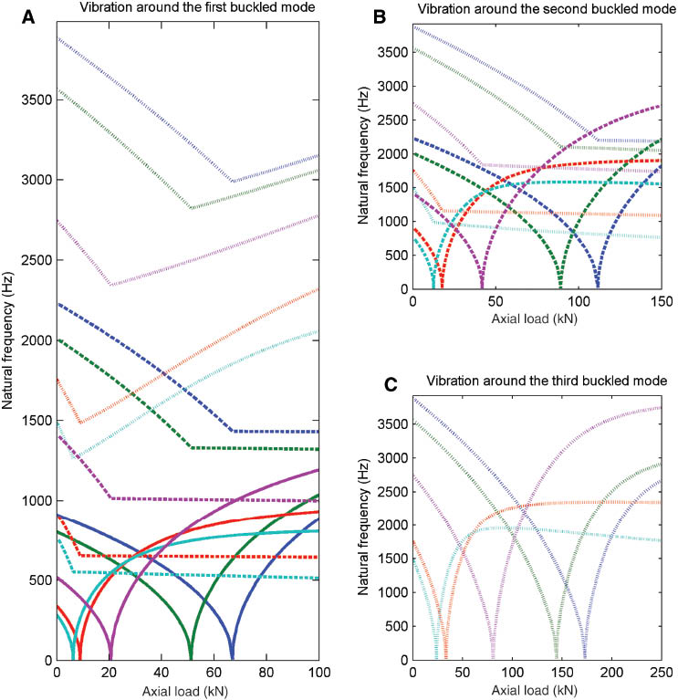
Figures 4–6 represent the variations of natural frequency versus the applied axial load around the first three buckled configurations of composite beams with unidirectional lay-up for SS, SC, and CC boundary conditions, respectively. Around the first buckled configuration, the results corresponding to the first three vibration modes are presented. For the second buckled configuration, the variations of natural frequencies for the second and third vibration modes are shown, and around the third buckled configuration, only the variation of frequencies of third vibration mode is illustrated. It is observed that by increasing the axial load, the natural frequency decreases in the prebuckling domain and approaches to zero, whereas it increases in the postbuckling domain. The intense decrease of natural frequency in the transition area from the prebuckling domain to the postbuckling domain is owing to the severe instability of the beam subjected to an axial load whose value is around the critical value of buckling load. In addition, it is seen that as the axial load increases, the slope of curves decreases in the postbuckling domain.
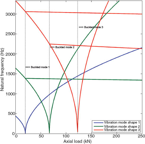
Variation of the natural frequency around the first three buckled configurations with the applied axial load for an SS beam with unidirectional lay-up.

Variation of the natural frequency around the first three buckled configurations with the applied axial load for an SC beam with unidirectional lay-up.

Variation of the natural frequency around the first three buckled configurations with the applied axial load for a CC beam with unidirectional lay-up.
Figures 4–6 reveal that two types of internal resonance might be activated between the vibration modes. The first type includes the internal resonances around the same buckled configurations, and the second one includes the internal resonances around different buckled configurations. If the corresponding mode shape of the natural frequency in the ith vibration mode around the jth buckled configuration is denoted by ϕij, from Figure 4 for an SS beam, it is seen that an internal resonance of the first type might be activated among ϕ11 and ϕ21 at N0≈113 KN. The important finding is that when the axial load exceeds N0≈113 KN, the vibration mode corresponding to the fundamental frequency shifts from 1 to 2. Thus, one may conclude that the beam subjected to axial loads with different magnitudes does not necessarily vibrate at its fundamental frequency in the first vibration mode, and similarly, the second vibration mode is not necessarily associated with the second frequency. Figure 6 for a CC beam also shows that there is a possibility for the activation of an internal resonance of the first type between ϕ11 and ϕ21 at N0≈181 KN, at which the mode of fundamental frequency is changed from 1 to 2. However, from Figure 5, it is observed that unlike the beams under SS and CC boundary conditions, there is no internal resonance of the first type in the graph of an SC beam, and accordingly the path of the first vibration mode around the first buckled configuration is always associated with the fundamental frequency. As shown in Figures 4–6, many internal resonances of the second type might also be activated among the vibration modes. For example, from Figure 6 for a CC beam, an interesting internal resonance between three modes of ϕ11, ϕ21, and ϕ33 might be activated at N0≈189 KN. Moreover, Figures 4 and 5 indicate that there is a possibility for the activation of internal resonances of the second type between ϕ11 and ϕ22 at N0≈83 KN and N0≈115 KN for SS and SC beams, respectively.
The effect of the lay-up configuration on the vibrations of buckled composite beams in both prebuckling and postbuckling domains is shown in Figures 7–9 for SS, SC, and CC boundary conditions, respectively. The colors of the curves in these figures are the same as those used in Figures 1–3 for the type of laminate. Also, the first three vibration modes are indicated by solid, dashed, and dotted lines, respectively. One can find that for all types of boundary conditions and for all vibration modes, the natural frequency in the prebuckling domain increases as the composite beam becomes stiffer. As an example, from Figures 1–3, it was observed that the composite beams with unidirectional lay-up have the maximum value of critical buckling load. Moreover, according to Figures 7–9, one can see that the natural frequencies of the composite beams with unidirectional lay-up in the prebuckling domain are larger than those of composite beams with other laminates. However, it is observed that the vibration of buckled beams in the postbuckling domain is more complicated than that in the prebuckling domain so that there is no such apparent relation between the lay-up configuration and natural frequency in the postbuckling domain. For example, the natural frequencies corresponding to ϕ11 in the postbuckling domain decrease with the increase of the stiffness of the SS beam, while the variation of natural frequencies of ϕ11 for SC and CC beams with the stiffness is dependent on the value of axial load. Also, in the case of the SS beam, in contrast to the natural frequencies of ϕ11 which decrease with the increase of the beam’s stiffness, the natural frequencies of ϕ21 increase as the beam becomes stiffer.

Variation of the natural frequency around the first three buckled configurations with the applied axial load for different laminates of an SS beam.

Variation of the natural frequency around the first three buckled configurations with the applied axial load for different laminates of an SC beam.
Variation of the natural frequency around the first three buckled configurations with the applied axial load for different laminates of a CC beam.
8 Conclusion
In this paper, a numerical solution strategy was proposed to study the postbuckling and vibrations of symmetrically and unsymmetrically composite Timoshenko beams undergoing postbuckling. First, the governing equations and associated boundary conditions were derived using the Hamilton principle. Based on the GDQ method, a set of differential operators was introduced with the aim of discretizing the governing equations and corresponding boundary conditions. The pseudo-arc-length method was used to solve the postbuckling problem. Thereafter, the problem of free vibration around the first three buckled configurations was solved as an eigenvalue problem via the solution obtained from the nonlinear problem in the previous step. Based on the numerical results, the following conclusions can be stated:
The lay-up configuration significantly affects the critical buckling load and postbuckling response of composite beams, and hence the beam behavior can be controlled by the appropriate lay-up configuration of the laminate. This conclusion is helpful for the design of composite beams.
As the applied axial load becomes larger, the natural frequency in the prebuckling domain and in the postbuckling domain, respectively, tends to decrease and increase. The drastic reduction of natural frequency in the transition area from the prebuckling domain to the postbuckling domain is due to the instability of the structure under the axial load around the critical buckling load.
There is a possibility for the activation of internal resonances between vibration modes around the same buckled configurations as well as different buckled configurations. When the frequency curves intersect each other around the same buckled configurations, the vibration mode corresponding to the fundamental frequency might be changed.
The natural frequency in the prebuckling domain increases as the composite beam becomes stiffer, while there is no specific relation between the lay-up configuration and natural frequency of composite beams in the postbuckling domain.
References
[1] Zhang Z, Taheri F. Composites: Part B 2003, 34, 391–398.10.1016/S1359-8368(02)00134-8Search in Google Scholar
[2] Ozturk H, Sabuncu M. Compos. Sci. Technol. 2005, 65, 1982–1995.10.1016/j.compscitech.2005.03.004Search in Google Scholar
[3] Aydogdu M. Compos. Sci. Technol. 2007, 67, 1096–1104.10.1016/j.compscitech.2006.05.021Search in Google Scholar
[4] Sapountzakis EJ, Tsiatas GC. Eng. Struct. 2007, 29, 675–681.10.1016/j.engstruct.2006.06.010Search in Google Scholar
[5] Gupta RK, Gunda JB, Janardhan GR, Rao GV. Compos. Struct. 2010, 92, 1947–1956.10.1016/j.compstruct.2009.12.010Search in Google Scholar
[6] Baghani M, Jafari-Talookolaei RA, Salarieh H. Appl. Math. Model. 2011, 35, 130–138.10.1016/j.apm.2010.05.012Search in Google Scholar
[7] Emam SA. Compos. Struct. 2011, 94, 24–30.10.1016/j.compstruct.2011.07.024Search in Google Scholar
[8] Vosoughi AR, Malekzadeh P, Banan Ma R, Banan Mo R. Int. J. Non-Linear Mech. 2012, 47, 96–102.10.1016/j.ijnonlinmec.2011.11.009Search in Google Scholar
[9] Vo TP, Thai HT. Int. J. Mech. Sci. 2012, 62, 67–76.10.1016/j.ijmecsci.2012.06.001Search in Google Scholar
[10] Ghayesh MH, Amabili M. Int. J. Mech. Sci. 2013, 68, 76–91.10.1016/j.ijmecsci.2013.01.001Search in Google Scholar
[11] Kisa M. Compos. Sci. Technol. 2004, 64, 1391–1402.10.1016/j.compscitech.2003.11.002Search in Google Scholar
[12] Shu D, Della CN. Int. J. Mech. Sci. 2004, 46, 509–526.10.1016/j.ijmecsci.2004.05.008Search in Google Scholar
[13] Dong XJ, Meng G, Li HG, Ye L. Mech. Res. Commun. 2005, 32, 572–581.10.1016/j.mechrescom.2005.02.014Search in Google Scholar
[14] Çalım FF. Compos. Struct. 2009, 88, 413–423.10.1016/j.compstruct.2008.05.001Search in Google Scholar
[15] Arvin H, Sadighi M, Ohadi AR. Compos. Struct. 2010, 92, 996–1008.10.1016/j.compstruct.2009.09.047Search in Google Scholar
[16] Ghayesh MH, Yourdkhani M, Balar S, Reid T. Appl. Math. Comput. 2010, 217, 545–556.10.1016/j.amc.2010.05.088Search in Google Scholar
[17] Kim JS, Wang KW. ASME J. Vib. Acoust. 2010, 132, 041003.Search in Google Scholar
[18] Gunda JB, Gupta RK, Janardhan GR, Rao GV. Compos. Struct. 2011, 93, 870–879.10.1016/j.compstruct.2010.07.006Search in Google Scholar
[19] Ghayesh MH. Acta Mech. Solida Sinica 2011, 24, 373–382.10.1016/S0894-9166(11)60038-4Search in Google Scholar
[20] Jafari-Talookolaei RA, Abedi M, Kargarnovin MH, Ahmadian MT. Int. J. Mech. Sci. 2012, 65, 97–104.10.1016/j.ijmecsci.2012.09.007Search in Google Scholar
[21] Nayfeh AH, Emam SA. Nonlinear Dyn. 2008, 54, 395–408.10.1007/s11071-008-9338-2Search in Google Scholar
[22] Emam SA, Nayfeh AH. Compos. Struct. 2009, 88, 636–642.10.1016/j.compstruct.2008.06.006Search in Google Scholar
[23] Ghayesh MH, Amabili M. Comput. Struct. 2012, 112–113, 406–421.10.1016/j.compstruc.2012.09.005Search in Google Scholar
[24] Ke LL, Yang J, Kitipornchai S. Meccanica 2010, 45, 743–752.10.1007/s11012-009-9276-1Search in Google Scholar
[25] Shu C. Differential Quadrature and Its Application in Engineering. Springer: London, 2000.10.1007/978-1-4471-0407-0Search in Google Scholar
[26] Keller HB. In Proc. Advanced Sem., University of Wisconsin, Madison, WI, 1976, Academic Press: New York, pp. 359–384.Search in Google Scholar
©2016 by De Gruyter
This article is distributed under the terms of the Creative Commons Attribution Non-Commercial License, which permits unrestricted non-commercial use, distribution, and reproduction in any medium, provided the original work is properly cited.
Articles in the same Issue
- Frontmatter
- Review
- The behaviour of aluminium matrix composites under thermal stresses
- Original articles
- Preparation and characterization of graphite/resin composite bipolar plates for polymer electrolyte membrane fuel cells
- Synergistic effect of carbon nanotubes in combination with magnesium hydroxide on the flame retardant poly(ethylene-co-vinyl acetate)
- Preparation and characterization of nano biphasic calcium phosphate/poly-L-lactide composite scaffold
- Durability study of ramie fiber fabric reinforced phenolic plates under humidity conditions
- Synthesis and molecular dynamics simulation of hyperbranched poly(amine-ester)/neodymium nanocomposites
- Investigation on wear properties of AZ31-MWCNT nanocomposites fabricated through mechanical alloying and powder metallurgy
- Probabilistic analysis of a thermosetting pultrusion process
- Analysis of shrinkage and creep behaviors in polymer-coated lightweight concretes
- Investigation of optimum cutting parameters and tool radius in turning glass-fiber-reinforced composite material
- Buckling and vibration analyses of composite laminates with weak interfaces by a coupled meshfree and finite element method
- Free vibration and postbuckling of laminated composite Timoshenko beams