The dynamics of prey–predator model with global warming on carrying capacity and wind flow on predation

1 Introduction

The prey-predator models are vital to understanding the relationship between biological populations and have drawn a lot of interest in mathematical biology. The dynamics of population models are affected by many different natural phenomena, including population size and age distribution. Prey–predator models with chaotic and limit cycle dynamics have received the majority of attention in the study on particular interactions [1]. Although many researchers have employed time as a continuous function in models [2], 3], discrete-time models [4], 5] have received less attention. These discrete-time models may be used to represent the nonlinear dynamics and chaotic behavior of populations of non-overlapping organisms, such as annual plants or insect populations with a single generation every year. To better understand the dynamics of the predator–prey system, several publications have been published [6], 7]. Mondal et al. [8] scrutinised the dynamic behaviour of a predator–prey model that incorporated the impacts of both fear and increased food. They investigated the stability characteristics of various equilibrium points and the presence of a Hopf bifurcation. In a predator–prey model where predation follows the Beddington-DeAngelis functional response, Pal et al. [9] discussed the effect of fear. They studied bifurcation, stability, and persistence. Ghosh et al. [10] investigated the memory impact in the ecological system using a fractional-order, eco-epidemiological model that included the effects of fear, treatment, and hunting cooperation. Deriving the infinitesimal generators of the Lie group symmetries is the first step in the analysis. Next, the algebraic structure of the equation’s symmetries in [11] is examined by building a commutator table and an adjoint table. In [12], the authors present a new pollinator model that includes two pollinator species (Vespa orientalis and honey bees) and flowering plants. The densities of flowering plants were thought to be influenced by the rates at which V. orientalis and honey bees visited the flowers. An effective technique for determining symmetry in nonlinear equations, Lie group theory, is used by the authors in [13] to investigate the simplified Ostrovsky equation. Finding infinitesimal generators is the first step in the process, after which adjoint and commutator tables are built to investigate the connections between the generators. A predator–prey model that takes into account memory effects, fear of predators, and the consequences of climate change is presented in the paper [14]. The effects of climate change are depicted using an exponential decay function. The non-dissipative instance of the strain wave equation’s structure, which takes into consideration numerous dimensions within microcrystalline structures, determines how waves are transmitted in microcrystalline materials, according to the research [15]. The dynamics of a discrete-time predator–prey model that was developed from a continuous framework are examined by the authors in [16], incorporating elements like moonlight, water resources, refuge availability, and prey alertness. The authors of the paper [17] investigate the nonlinear Helmholtz equation using a variety of techniques. First, they use bifurcation analysis, which is illustrated by phase portraits, to examine the system’s dynamic behavior. A mathematical model for the effects of dust pollution and climate change on plant biomass dynamics is presented in the Hakeem and et al. [18] paper. The suggested model is explained in detail. A mathematical model for the impact of dust storms on plant biomass dynamics is presented in Ahmed and his colleagues’ [10] work. The existence, uniqueness, and boundedness of the system’s solution are examined in Majeed and colleagues’ [19] analysis and proposal of the Omnivore–predator–prey model, which includes the II-Holling functional response to the interaction between Predator–Prey and the Nonlinear functional response to the interaction between Omnivore–Prey. The intended model is explained in detail. Assuming that certain beneficial bacteria undergo deleterious mutations as a result of antibiotic exposure, the study’s publication [20] offers a mathematical model explaining how gut microorganisms interact with probiotics and antibiotics. Al Nuaimi and Jawad [21] The dynamics of interactions between four species are examined in this research. Two predators and two competitive prey make up the system; the first predator preys on the first prey. A three-species food chain model that takes into account interactions between small fish, remora fish, and giant fish has been created for the study [22]. The Holling type II functional response is thought to be the mechanism via which huge fish eat little fish.

Global warming is the term used to describe the steady rise in the planet’s average temperature. Although there has been a warming trend for some time, it has accelerated significantly in the last century due to the use of fossil fuels. The number of people on the planet has grown together with the amount of fossil fuels burned [23], [24], [25]. The “greenhouse effect” is the outcome of burning fossil fuels like coal, oil, and natural gas in Earth’s atmosphere [26]. The greenhouse effect is the result of solar radiation entering the atmosphere and reflecting off objects, keeping heat from escaping back into space. Gases released during the combustion of fossil fuels prevent heat from exiting the atmosphere [27]. Among these greenhouse gases are carbon dioxide, water vapor, methane, nitrous oxide, and chlorofluorocarbons. As the name suggests, world warming is the gradual rise in global average temperature brought on by an excess of heat in the atmosphere [28]. A new issue brought on by global warming is climate change. Despite their sometimes synonyms, these phrases have distinct meanings. The phrase “climate change” refers to changes in the weather and growth seasons around the world. It also discusses how warmer oceans and the melting of glaciers and ice sheets cause sea levels to increase. Global warming-related climate change poses a threat to life as we know it by bringing with it extreme weather patterns and widespread flooding. The implications of global warming on Earth are still being studied [29].

About 9 % of all CO₂ emissions come from the animal agriculture industry. These emissions are mostly caused by the production of fertilizer for feed crops, energy costs on farms, the transportation of feed, the processing and transportation of animal products, and changes in land use. As per [30], the combustion of fossil fuels to produce fertilisers for feed crops has the potential to emit 41 million metric tonnes of CO₂ every year. Animal feed on farms is grown using massive amounts of artificial nitrogenous fertilizer, mostly made of corn and soybeans. Most of this fertiliser is produced in companies that use fossil fuels for energy production. Every year, 100 million metric tons of artificial fertilizer for feed crops are produced using the Haber-Bosch process, which yields ammonia and then turns it into nitrogen-based fertilizer. Fossil fuels used for intense confinement operations may release an extra 90 million metric tons of CO₂ annually. Compared to larger, more expansive, or pasture-based farms, these industrial enterprises utilize a lot less energy. While heating, cooling, and ventilation systems consume a significant amount of energy during intensive confinement operations, feed crop production accounts for over half of the energy used. This includes the production of seed, pesticides, and herbicides, as well as the fossil fuels required to run farm machinery [30]. Here is a group of effects that global warming may cause, which negatively affects the ecosystem. Perhaps the most important of these effects is the following [31]:

1. Tracking the Earth’s sea level rise brought on by the melting of Antarctic and Arctic ice. It should be mentioned that this raises the sea and ocean levels, which could result in low-lying islands and coastal cities drowning [32].

2. In addition to causing many species to go extinct, the phenomena of global warming also causes many other species to migrate. This is because some organisms migrated and went extinct since they were unable to adapt to the harsh climate factors [33].

3. In addition to the loss of crops due to storms, hurricanes, and increased rainfall in some areas, numerous calamities that affect agriculture can result in the loss of numerous forests.

4. Due to exposure to periods of extreme heat and drought, the phenomenon of desertification has spread over wide areas in numerous places.

5. Increased likelihood of forest fires as a result of drought in some areas and a lack of precipitation in others [34].

The structure of the paper is as follows: In Section 2, the mathematical model is developed. In Section 3, the positivity and boundedness of the model solutions have been examined. The equilibrium points of the model are determined in Section 4. Section 5 contains the equilibrium points where the model’s stability has been verified. In Section 6, the topic of Hopf bifurcation was examined. In Section 7, some results of numerical simulation are shown. The final portion contains the model analysis results.

2 Model formulation

We have built a model of how prey and predators interact in the context of wind and global warming in this research. This concept is derived from actual life. The densities of global warming, prey, and predator at time t are denoted by N(t), P(t), and g(t), respectively. To build the model, we have made the following assumptions:

1. In the absence of predators and global warming, prey is assumed to grow logistically. It is considered that the predator’s fear has a detrimental effect on the prey’s rate of growth [40]. Global warming is also considered to reduce the carrying capacity of prey species [41], 42].

2. The predator consumes prey using a modified Holling type II functional response [43], and it is assumed that the wind flow affects [44] how frequently the predator attacks prey. Predator collaboration while hunting is assumed to have an impact on the predation process as a whole [45].

3. Moreover, the predator growth model also accounts for the global warming effect, which results in decreased predator growth [46]. So, it is considered that a constant amount of additional food [47] is provided to the predator, denoted by the biomass L.

For their existence, predators are dependent on less dynamic prey. To model the interaction between prey and predator, a generalized Holling type II interaction is used. Our hypothesis states that as the density of the predator population rises, so does the encounter rate between the predator population and the prey. So, by changing the encounter rate to ψ(P) = α + βP, where α is the attack rate of prey and β is the measure of the level of predator cooperation while hunting. By including the effects of wind flow in the consumption of prey by predator with hunting cooperation among predators, the functional form becomes (1 + w)(α + βP)NP, which represents the effective hunting success rate. Again, the term 1 + h(1 + w)(α + βP)N accounts for the additional handling time or difficulty factor h. Then we can construct the following new modified Holling type II functional response

Currently, the following modified Leslie-Gower type functional form is taken into consideration for the change in predator species density over time:

where r ₂, ξ ₂, and L are the growth rate of predator, global warming effect on the growth of predator and the alternate food source for predator respectively.

Next, it is assumed that environmental pollution and gas emissions from factories, laboratories, and others contribute to expanding global warming at a rate a ₁, where prey and predators contribute to global warming at a rate a ₂ and a ₃ respectively. It is assumed that it is possible to reduce the rate of global warming by implementing natural and industrial policies at a rate μ. Then the change of global warming with respect to time may become the following form:

As per the above mentioned assumptions, we have developed the model as follows:

with initial conditions

The description of the model parameters are given in Table 1.

3 Positiveness and boundedness

In this section, we have examined the boundedness and positivity of the solutions to the model.

4 Equilibrium points

In this section, all possible equilibrium points of the model are evaluated as follows:

1. E 0 = k 1 μ − ξ 1 a 1 μ + ξ 1 a 2 , 0 , a 1 + a 2 k 1 μ + ξ 1 a 2 ) which exists when k ₁ μ > ξ ₁ a ₁. The inequality k ₁ μ > ξ ₁ a ₁ guarantees that the population’s growth or recruitment rate exceeds the combined adverse impacts of mortality and interactions (such as competition or predation) that cause the population to shrink.

2. E 1 = 0 , P 1 , a 1 + a 3 P 1 μ where P ₁ is a root of ξ ₂ a ₃ P ² + (μ + ξ ₂ a ₁)P − r ₂ Lμ = 0 which has the root P 1 = − ( μ + ξ 2 a 1 ) + ( μ + ξ 2 a 1 ) 2 + 4 ξ 2 a 3 r 2 L μ 2 ξ 2 a 3 , its clear that P ₁ is positive real root.

3. E* = (N*, P*, g*), we can figure it out by solving the system below:

   (3) r 1 1 + a P 1 − N k 1 − ξ 1 g − ( 1 + w ) ( α + β P ) P 1 + h ( 1 + w ) ( α + β P ) N = 0 r 2 1 + ξ 2 g − P e 1 N + L = 0 a 1 + a 2 N + a 3 P − μ g = 0

Substituting g* in the first and second equations of (3), we have (N*, P*) is the positive intersection point of the following isoclines:

As N → 0, we have

Note that N Δ 1 and N Δ 2 are a roots of the following polynomials respectively

It is clear that N Δ 1 and N Δ 2 = − ( μ + ξ 2 a 1 ) + ( μ + ξ 2 a 1 ) 2 + 4 ξ 2 a 3 r 2 L μ 2 ξ 2 a 3 are unique due to Descartes’s rule of signs and assume that those roots are positive. Also, we take for granted that the next two requirements are met:

So, the slope of Δ₁(N, P) is negative.It is clear that the two isoclines Δ₁(N, P) and Δ₂(N, P) uniquely cross at a point (N*, P*) in the positive N − P plane. Consequently, the interior equilibrium point is real and is defined as E* = (N*, P*, g*). The following result is obtained.

5 Stability analysis

This section looks into the local asymptotic stability of system (1)’s equilibria. By computing the Jacobian matrix at the equilibria, the stability of each of them is analyzed through the roots of the characteristic equation assessed with it. To accomplish this, let J _E (N, P, g) be the Jacobian matrix calculated at any equilibrium E(N, P, g),

where,

then, by calculating, it can be concluded the characteristic equation for J _E (N, P, g) is formulated as

where,

Furthermore, let Δ _E  = Γ₁Γ₂ − Γ₃. Now the following theorems are given to analyze the local stability at steady states E*, E ₁, and E ₀.

6 Hopf bifurcation

Hopf bifurcations are helpful in detecting oscillatory behavior in biological models and offer important details regarding the stability of the solution near equilibrium; ecologically, a stable periodic solution suggests that the model exhibits continuous oscillatory behavior. So, in this section, we focus on the circumstances in which a set of periodic solutions in system (1) bifurcates around the positive steady state point E*, i.e., the potential for a change in a specific parameter to cause a qualitative shift (Hopf bifurcation) in the dynamical behavior of system (1). In the next theorem, we perceive that system (1) undergoes an interior equilibrium point-centered Hopf bifurcation at the threshold value μ = μ _h .

7 Numerical results

We have used the following set of fictitious parameter values in our numerical simulations:

It’s crucial to remember that no experimental real-world data was used to determine these figures. These parameter values are not intended to depict a particular real-world case, even if they were influenced by references in the body of current research [38], [39], [40]. Rather, they were selected to illustrate and assess the theories and notions presented in the theoretical framework.

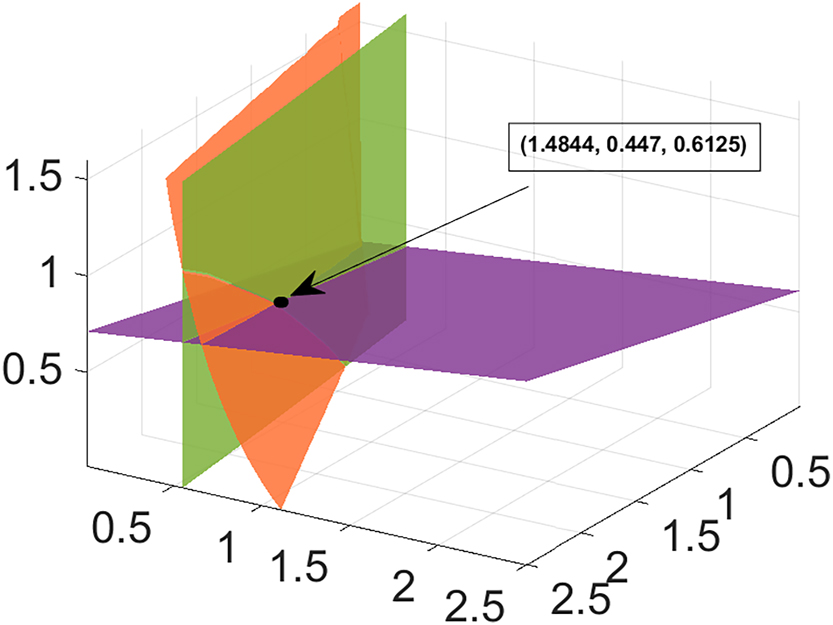
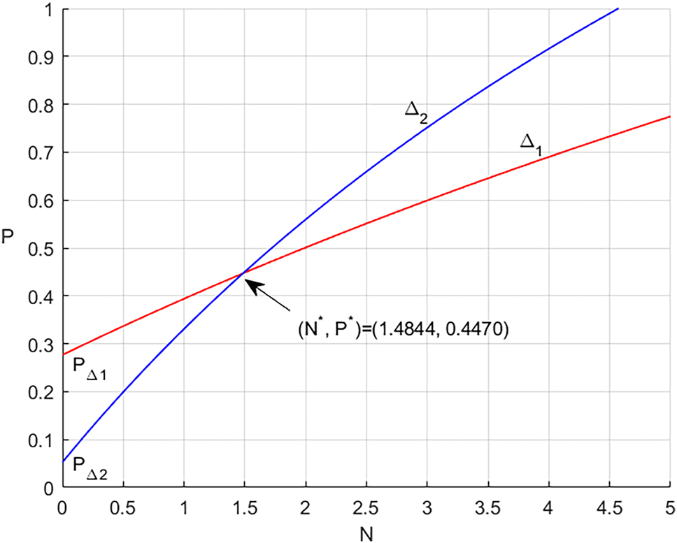
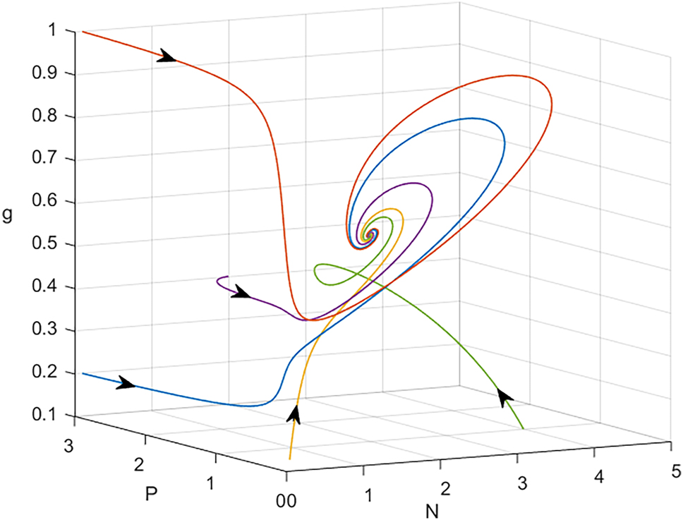
It is difficult to determine the existence of coexistence equilibrium E* using analytical calculations. Therefore, we first confirm the presence of coexistence equilibrium numerically. To do this, we plot the homogeneous model (1) system in N − P − g space, as shown in Figure 1. The image makes it evident that the coexistence equilibrium, or E*, is where three planes join at the pink color at the positive octant. Again, with the same parameter values utilized in Figure 1, in Figure 2, in N − P space the two isoclines Δ₁ and Δ₂ have been plotted. It is found they intersect at a unique interior point (N*, P*) = (1.4844, 0.4470). After that, this outcome is used in equation (4), which yields g* = 0.6132. Moreover, Figure 3 presents a graphical representation of the phase portrait diagrams of system (1) for a number of initial values of N*, P*, and g*. It follows that every solution that begins at one of these initial points converges asymptotically to the coexistence solution (1.4844, 0.447, 0.6132).

Figure 1:

Coexistence equilibrium point E* = (N*, P*, g*) with data set (18) except r ₁ = 0.7.

Figure 2:

Isocline diagram for model (1) in N − P space with data set (18) except r ₁ = 0.7.

Figure 3:

Phase portrait of the model (1) for different initial values, also with the data set (18) except r ₁ = 0.7 converge asymptotically to the coexistence equilibrium point (1.4844, 0.447, 0.6132).

On the other hand, three sub-figures are plotted in Figure 4 with three data sets to show the effect of increasing some parameter values such as Wind flow w, Conversion efficiency e ₁, and Alternative prey concentration L on the stability of prey-free steady state point. Due to the data used in each sub-figure the Jacobin matrix (8) has three characteristic roots. First with data set used in Figure 4(a), J E 1 has λ ₁ = −0.0974, λ ₂ = −2.584 and λ ₃ = −0.5137. While with data set used in Figure 4(b), J E 1 has λ ₁ = −0.0149 and λ _2,3 = −0.5432 ± 0.0631i. Further, with data set used in Figure 4(c), J E 1 has λ ₁ = −0.0589, λ ₂ = −0.7790 and λ ₃ = −0.5098 ± 0.0631i. So, in this case, the solution goes asymptotically to a prey-free steady point. Therefore, based on this figure, it can be concluded that increasing these parameter values might affect the model’s stability.

Figure 4:

Time series for model (1) with data set (18), except at (a) w = 4 & e ₁ = 0.4; (b) w = 4 & L = 0.4; and (c) w = 16, show that the solutions converge asymptotically to prey-free steady point E ₁.

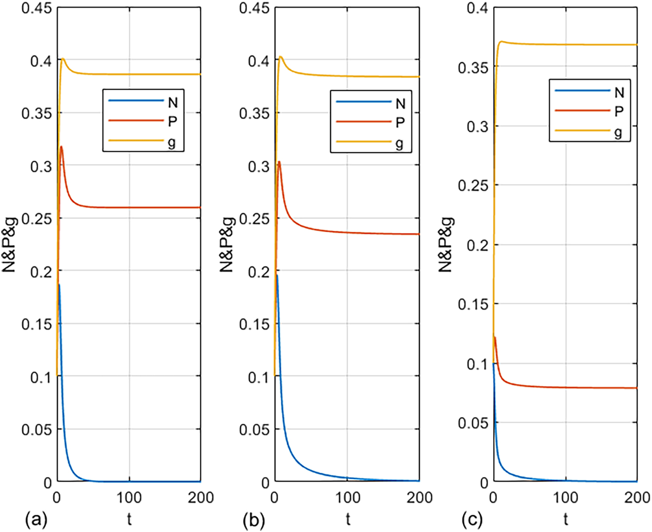
Figure 5 presents the bifurcation diagram of model (1) with respect to the parameter a. The diagram indicates that as a varies from 0.1 to 0.8, the system undergoes a Hopf bifurcation. For 0.1 ≤ a < 0.4763, the predator–prey dynamics exhibit sustained oscillations, whereas for 0.4763 < a ≤ 0.8, the populations tend to settle into a stable steady state. Increasing the parameter a, which reflects the prey’s fear of predators, appears to enhance the system’s stability. This stabilizing effect arises because prey individuals that are more adept at evading predators face a reduced risk of predation, thereby supporting the long-term persistence of the prey population.

Figure 5:

Bifurcation diagram of model (1) with respect to a for the set of parametric values of (18) except e ₁ = 1.5, a ₁ = 0.18.

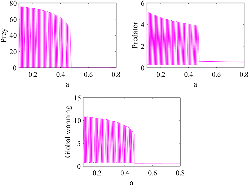
Figure 6 illustrates the bifurcation diagram of model (1) with respect to the parameter β. As β increases from 0.2 to 1.2, the diagram indicates that the system may undergo a Hopf bifurcation. Specifically, for 0.2 ≤ β < 0.32, the predator–prey populations tend to exhibit a stable steady state, whereas for 0.32 < β ≤ 1.2, the system displays unstable dynamics. These findings suggest that greater cooperation among predators, represented by higher values of β, may lead to increased instability in the model.

Figure 6:

Bifurcation diagram of model (1) with respect to β for the set of parametric values (18) except ξ ₂ = 0.9, e ₁ = 0.7.

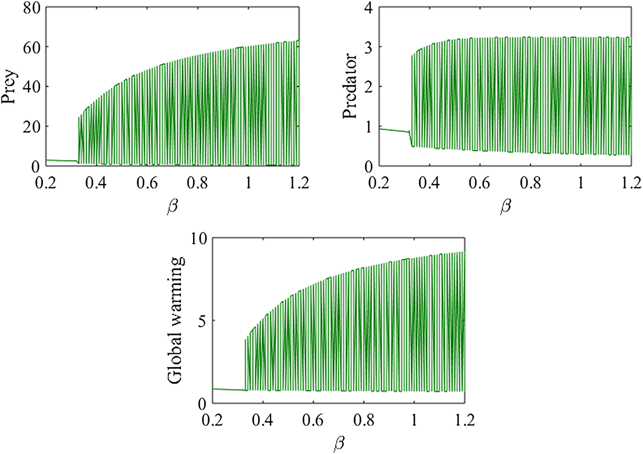
Figure 7 presents the bifurcation diagram of model (1) with respect to the parameter e ₁. The diagram shows that as e ₁ varies from 0.6 to 2.0, the system may undergo a Hopf bifurcation. Specifically, for 0.6 ≤ e ₁ < 0.698 and 1.328 < e ₁ ≤ 2.0, the predator–prey populations tend to remain at a stable steady state, whereas for 0.698 < e ₁ < 1.328, the system exhibits oscillatory dynamics. These results suggest that increasing the prey’s conversion efficiency enhances the stability of the model. When prey efficiently convert resources into biomass, their populations are less prone to dramatic fluctuations, reducing the likelihood of boom-and-bust cycles. This stability in prey populations can cascade through the food web, contributing to greater overall ecosystem stability.

Figure 7:

Bifurcation diagram of model (1) with respect to e ₁ for the set of parametric values (18).

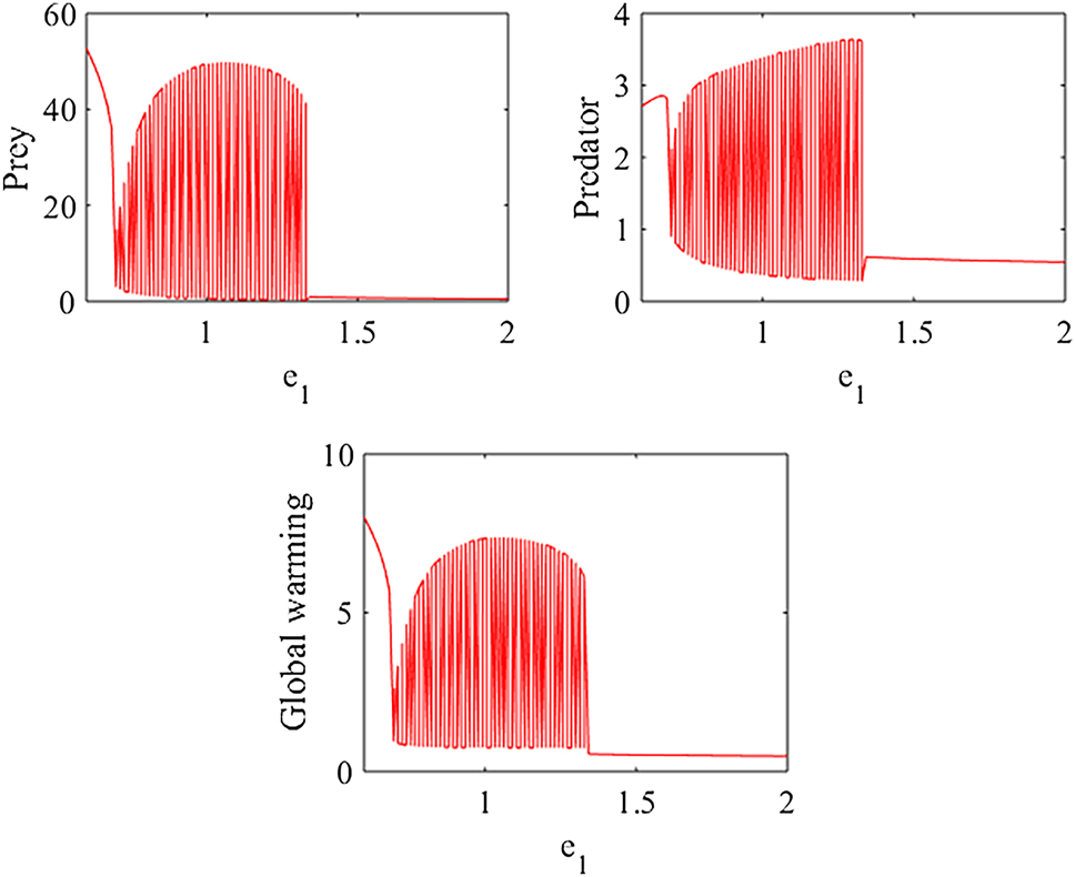
Figure 8 presents the bifurcation diagram of model (1) with respect to the parameter μ. The diagram indicates that as μ varies from 0.5 to 0.7, the system may undergo a Hopf bifurcation. Specifically, for 0.5 ≤ μ < 0.594, the predator–prey populations exhibit oscillatory behavior, while for 0.594 < μ < 0.7, the system tends to maintain a stable steady state. These findings suggest that reducing the effects of global warming through effective natural and industrial policies may help sustain stability in predator–prey dynamics. Natural strategies, such as afforestation, reforestation, and biodiversity conservation, can enhance carbon sequestration and ecosystem resilience. Industrial measures, including the transition to renewable energy, improvements in energy efficiency, and the adoption of carbon capture and storage technologies, can significantly mitigate greenhouse gas emissions, thereby promoting environmental stability.

Figure 8:

Bifurcation diagram of model (1) with respect to μ for the set of parametric values (18) except e ₁ = 0.7.

Figure 9 illustrates the bifurcation diagram of model (1) with respect to the parameter w. The diagram indicates that as w varies from 3.4 to 3.9, the system may undergo a Hopf bifurcation. Specifically, for 3.4 ≤ w < 3.495, the predator–prey populations tend to remain in a stable steady state, whereas for 3.495 < w ≤ 3.9, the system exhibits unstable or oscillatory dynamics. These results suggest that wind direction can influence the dynamics of the ecological system. By affecting the dispersion of scent molecules or the spatial distribution of prey organisms, changes in wind direction may indirectly modify predator–prey interactions. Such shifts could alter the movement patterns of both predators and prey, potentially causing fluctuations in predation rates and impacting the overall stability of the predator–prey system.

Figure 9:

Bifurcation diagram of model (1) with respect to w for the set of parametric values (18) ξ ₂ = 0.9.

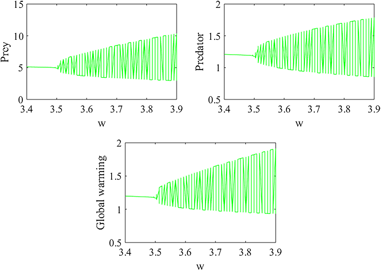
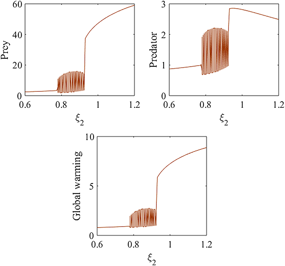
Figure 10 presents the bifurcation diagram of model (1) with respect to the parameter ξ ₂. The diagram shows that for 0.6 ≤ ξ ₂ < 0.774 and 0.93 ≤ ξ ₂ ≤ 1.2, the predator–prey populations tend to maintain a stable steady state, whereas for 0.774 < ξ ₂ < 0.93, the system exhibits unstable or oscillatory behavior. These findings suggest that global warming may reduce the carrying capacity of prey species, thereby affecting ecological stability. Rising temperatures and shifts in precipitation patterns can alter habitat suitability, reducing the availability of food and other critical resources. Additionally, increased heat stress can impair prey physiology, lower reproductive success, and drive changes in species distribution. Such impacts on prey populations may cascade through the food web, influencing the overall stability of predator–prey dynamics.

Figure 10:

Bifurcation diagram of model (1) with respect to ξ ₂ for the set of parametric values (18) except e ₁ = 0.7.

8 Conclusions

This research paper develops a mathematical model to study predator–prey dynamics between two interacting species under the influence of global warming. The model incorporates several ecological and environmental factors. Predator fear is assumed to be inversely related to the prey growth rate, while the carrying capacity of the prey population is considered to decline as global warming intensifies. Predators are assumed to cooperate in hunting prey, and their consumption of prey is influenced by wind direction. The predator growth rate is assumed to decrease with rising global temperatures, and predator populations are further reduced by intraspecific competition, which depends on the density of available prey. Global warming is modeled as increasing at a constant rate, with both predators and prey contributing to its rise, while various industrial and ecological measures are considered as potential means to mitigate it. The study examines the positivity and boundedness of solutions, evaluates multiple equilibrium points, and analyzes the system’s stability around these points. Based on this analysis, the following conclusions have been drawn:

1. Increasing prey fear of predators enhances system stability, shifting dynamics from oscillatory to a stable steady state.

2. Greater predator cooperation increases instability, leading to oscillatory dynamics beyond a threshold.

3. Higher prey conversion efficiency stabilizes the predator–prey system by reducing population fluctuations and preventing boom-and-bust cycles.

4. Mitigating global warming through natural (e.g., afforestation, reforestation) and industrial (e.g., renewable energy, carbon capture) policies can maintain stability in ecological interactions.

5. Changes in wind direction can indirectly affect predator–prey interactions by altering movement patterns and predation rates, potentially causing instability.

6. Global warming may lower the carrying capacity of prey species, which can destabilize the system by reducing resource availability and affecting prey survival and reproduction.

1. Only theoretical: By using fake or placeholder parameters, the model is not empirically calibrated, which compromises its validity and real-world applicability.

2. Data scarcity: Whether as a result of low resolution, inadequate sampling, or a lack of long-term datasets, ecological models typically suffer from a lack of data, which makes parameterization challenging and lowers predicted dependability.

3. Tractability is diminished by high complexity: While adding higher-order variables and nonlinearities (such modified functional responses) enhances dynamics, it also makes analysis more difficult and may result in equifinality, where several parameter choices fit equally well.

4. Uncertainty and structural sensitivity: Predictions may spread unacknowledged uncertainty (in parameters or model form). There are significant hazards associated with structural sensitivity, when little modifications to the model form produce differing results.

References

1. Kooij, RE, Zegeling, A. Qualitative properties of two-dimensional predator-prey systems. Nonlinear Anal 1997;29:693–715. https://doi.org/10.1016/s0362-546x(96)00068-5.Suche in Google Scholar
2. Maiti, AP, Dubey, B, Tushar, J. A delayed prey–predator model with Crowley–Martin-type functional response including prey refuge. Math Methods Appl Sci 2017;40:5792–809. https://doi.org/10.1002/mma.4429.Suche in Google Scholar
3. Jawad, S, Winter, M, Zeb, A. Stability analysis of excessive carbon dioxide gas emission model through following reforestation policy in low-density forest biomass. Baghdad Sci J 2024;22:1335–53. https://doi.org/10.21123/bsj.2024.11370.Suche in Google Scholar
4. Huang, J, Liu, S, Ruan, S, Xiao, D. Bifurcations in a discrete predator–prey model with nonmonotonic functional response. J Math Anal Appl 2018;464:201–30. https://doi.org/10.1016/j.jmaa.2018.03.074.Suche in Google Scholar
5. Singh, A, Elsadany, AA, Elsonbaty, A. Complex dynamics of a discrete fractional-order Leslie-Gower predator-prey model. Math Methods Appl Sci 2019;42:3992–4007. https://doi.org/10.1002/mma.5628.Suche in Google Scholar
6. Owolabi, K, Pindza, E. Mathematical and computational studies of fractional reaction–diffusion system modelling predator–prey interactions. J Numer Math 2018;26:97–110. https://doi.org/10.1515/jnma-2016-1044.Suche in Google Scholar
7. Hassell, MP. The dynamics of arthopod predator-prey systems. (MPB-13). Princeton: Princeton University Press; 2020, vol 13.10.12987/9780691209968Suche in Google Scholar
8. Mondal, S, Maiti, A, Samanta, GP. Effects of fear and additional food in a delayed predator–prey model. Biophys Rev Lett 2018;13:157–77. https://doi.org/10.1142/s1793048018500091.Suche in Google Scholar
9. Pal, S, Majhi, S, Mandal, S, Pal, N. Role of fear in a predator–prey model with Beddington–DeAngelis functional response. Z Naturforsch 2019;74:581–95. https://doi.org/10.1515/zna-2018-0449.Suche in Google Scholar
10. Ahmed, M, Jawad, S, Das, D, Boulaaras, SM, Osman, MS. Impact of dust storms on plant biomass: model structure and dynamic study. Alex Eng J 2025;126:605–22.10.1016/j.aej.2025.04.058Suche in Google Scholar
11. Chou, D, Boulaaras, SM, Abbas, M, Iqbal, I, Rehman, HU. Dynamics of solitons, lie symmetry, bifurcation, and stability analysis in the time-regularized long-wave equation. Int J Theor Phys 2025;64:66.10.1007/s10773-025-05935-5Suche in Google Scholar
12. Jawad, S, Thirthar, AA, Nisar, KS. The impact of climate change on flowering plants-bees-Vespa orientalis model. Results Control Optim 2025;20:100583.10.1016/j.rico.2025.100583Suche in Google Scholar
13. Chou, D, Boulaaras, SM, Rehman, HU, Iqbal, I, Abbas, M. Lie symmetries, soliton dynamics, bifurcation analysis and chaotic behavior in the reduced Ostrovsky equation. Rendiconti Lincei Sci Fis Nat 2024;36:257–75.10.1007/s12210-024-01294-1Suche in Google Scholar
14. Thirthar, AA, Alaoui, AL, Roy, S, Tiwari, PK. Fractional and stochastic dynamics of predator–prey systems: the role of fear and global warming. Eur Phys J B 2025;98:147.10.1140/epjb/s10051-025-00992-5Suche in Google Scholar
15. Chou, D, Boulaaras, SM, Rehman, HU, Iqbal, I, Ma, W. Multiple soliton and singular wave solutions with bifurcation analysis for a strain wave equation arising in microcrystalline materials. Mod Phys Lett B 2024;39:2550088.10.1142/S0217984925500885Suche in Google Scholar
16. Mokni, K, Thirthar, AA, Ch-Chaoui, M, Jawad, S, Abbasi, MA. Stability and bifurcation analysis in a novel discrete prey-predator system incorporating moonlight, water availability, and vigilance effects. Int J Dyn Control 2025;13:219.10.1007/s40435-025-01718-2Suche in Google Scholar
17. Iqbal, I, Boulaaras, SM, Althobaiti, S, Althobaiti, A, Rehman, HU. Exploring soliton dynamics in the nonlinear Helmholtz equation: bifurcation, chaotic behavior, multistability, and sensitivity analysis. Nonlinear Dyn 2025;113:16933–54. https://doi.org/10.1007/s11071-025-10961-3.Suche in Google Scholar
18. Hakeem, E, Jawad, S, Ali, AH, Kallel, M, Neamah, HA. How mathematical models might predict desertification from global warming and dust pollutants. MethodsX 2025;14:103259.10.1016/j.mex.2025.103259Suche in Google Scholar PubMed PubMed Central
19. Majeed, SJ, Naji, RK, Thirthar, AA. The dynamics of an omnivore-predator-prey model with harvesting and two different nonlinear functional responses. AIP Conf Proc 2019b;2096:020008.10.1063/1.5097805Suche in Google Scholar
20. Ahmed, M, Jawad, S. Bifurcation analysis of the role of good and bad bacteria in the decomposing toxins in the intestine with the impact of antibiotic and probiotics supplement. AIP Conf Proc 2024;3097:080033.10.1063/5.0209388Suche in Google Scholar
21. Al Nuaimi, M, Jawad, S. Modelling and stability analysis of the competitional ecological model with harvesting. Commun Math Biol Neurosci 2022;2022:47.Suche in Google Scholar
22. Thirthar, AA, Mahdi, ZA, Panja, P, Biswas, S, Abdeljawad, T. Mutualistic behaviour in an interaction model of small fish, remora and large fish. Int J Model Simul 2024b:1–14. https://doi.org/10.1080/02286203.2024.2392218.Suche in Google Scholar
23. Allan, RP, Arias, PA, Berger, S, Canadell, JG, Cassou, C, Chen, D, et al.. Intergovernmental panel on climate change (IPCC). Summary for policymakers. In: Climate change 2021: the physical science basis. Contribution of working group I to the sixth assessment report of the intergovernmental panel on climate change. Cambridge, UK and New York, USA: Cambridge University Press; 2023:3–32 pp.10.1017/9781009157896.001Suche in Google Scholar
24. Lee, H, Calvin, K, Dasgupta, D, Krinner, G, Mukherji, A, Thorne, P, et al.. IPCC, 2023: climate change 2023: synthesis report, summary for policymakers. Contribution of working groups I, II and III to the sixth assessment report of the intergovernmental panel on climate change [Core Writing Team, H. Lee and J. Romero (eds.)]. Geneva, Switzerland: IPCC; 2023.Suche in Google Scholar
25. Wuebbles, D, Fahey, D, Takle, E, Hibbard, K, Arnold, J, DeAngelo, B, et al.. Climate science special report: fourth national climate assessment (NCA4). Washington, DC, USA: U.S. Global Change Research Program; 2017, vol I.10.7930/J0DJ5CTGSuche in Google Scholar
26. Chiari, L, Zecca, A. Constraints of fossil fuels depletion on global warming projections. Energy Policy 2011;39:5026–34. https://doi.org/10.1016/j.enpol.2011.06.011.Suche in Google Scholar
27. Stephens, GL, L’Ecuyer, T. The Earth’s energy balance. Atmos Res 2015;166:195–203.10.1016/j.atmosres.2015.06.024Suche in Google Scholar
28. Setzer, J, Higham, C. Global trends in climate change litigation: 2022 snapshot. London: Grantham Research Institute on Climate Change and the Environment and Centre for Climate Change Economics and Policy, London School of Economics and Political Science; 2022.Suche in Google Scholar
29. Soutter, ARB, Mõttus, R. “Global warming” versus “climate change”: a replication on the association between political self-identification, question wording, and environmental beliefs. J Environ Psychol 2020;69:101413.10.1016/j.jenvp.2020.101413Suche in Google Scholar
30. Steinfeld, H, Gerber, P, Wassenaar, TD, Castel, V, De Haan, C. Livestock’s long shadow: environmental issues and options. Rome, Italy: Food & Agriculture Org; 2006.Suche in Google Scholar
31. Dincer, I, Colpan, CO, Kadioglu, F, editors. Causes, impacts and solutions to global warming. New York, NY, USA: Springer Science & Business Media; 2013.10.1007/978-1-4614-7588-0Suche in Google Scholar
32. Magnan, AK, Garschagen, M, Gattuso, JP, Hay, JE, Hilmi, N, Holland, EA, et al.. Low-lying islands and coasts. In: Pörtner HO, Roberts DC, Masson-Delmotte V, Zhai P, Tignor M, Poloczanska E, et al., editors. IPCC special report on the ocean and cryosphere in a changing climate. Cambridge, UK and New York, NY, USA: Cambridge University Press; 2019:657–74 pp.Suche in Google Scholar
33. Species, M, Change, C. Impacts of a changing environment on wild animals. In: UNEP/cms convention on migratory species and DEFRA. Bonn, Germany: United Nations Environment Programme (UNEP)/CMS Secretariat; 2006.Suche in Google Scholar
34. Richardson, D, Black, AS, Irving, D, Matear, RJ, Monselesan, DP, Risbey, JS, et al.. Global increase in wildfire potential from compound fire weather and drought. npj Clim Atmos Sci 2022;5:23. https://doi.org/10.1038/s41612-022-00248-4.Suche in Google Scholar
35. Thirthar, AA, Panja, P, Khan, A, Alqudah, MA, Abdeljawad, T. An ecosystem model with memory effect considering global warming phenomena and an exponential fear function. Fractals 2023;31:2340162. https://doi.org/10.1142/s0218348x2340162x.Suche in Google Scholar
36. Thirthar, AA, Sk, N, Mondal, B, Alqudah, MA, Abdeljawad, T. Utilizing memory effects to enhance resilience in disease-driven prey-predator systems under the influence of global warming. J Appl Math Comput 2023;69:4617–43. https://doi.org/10.1007/s12190-023-01936-x.Suche in Google Scholar
37. Panja, P, Kar, T, Jana, DK. Impacts of global warming on phytoplankton–zooplankton dynamics: a modelling study. Environ Dev Sustainability 2024;26:1–19. https://doi.org/10.1007/s10668-023-04430-3.Suche in Google Scholar
38. Thirthar, AA, Jawad, S, Abbasi, MA. The modified predator–prey model response to the effects of global warming, wind flow, fear, and hunting cooperation. Int J Dyn Control 2024;13:3.10.1007/s40435-024-01504-6Suche in Google Scholar
39. Thirthar, AA, Jawad, S, Panja, P, Mukheimer, A, Abdeljawad, T. The role of human shield in prey, crop-raiders and top predator species in southwestern Ethiopia’s coffee forests: a modeling study. J Math Comput SCI-JM 2025;36:333–51. https://doi.org/10.22436/jmcs.036.03.08.Suche in Google Scholar
40. Sheriff, MJ, Krebs, CJ, Boonstra, R. The sensitive hare: sublethal effects of predator stress on reproduction in snowshoe hares. J Anim Ecol 2009;78:1249–58. https://doi.org/10.1111/j.1365-2656.2009.01552.x.Suche in Google Scholar PubMed
41. Deutsch, CA, Tewksbury, JJ, Huey, RB, Sheldon, KS, Ghalambor, CK, Haak, DC, et al.. Impacts of climate warming on terrestrial ectotherms across latitude. Proc Natl Acad Sci 2008;105:6668–72. https://doi.org/10.1073/pnas.0709472105.Suche in Google Scholar PubMed PubMed Central
42. Wilmers, CC, Post, E, Hastings, A. The anatomy of predator–prey dynamics in a changing climate. J Anim Ecol 2007;76:1037–44. https://doi.org/10.1111/j.1365-2656.2007.01289.x.Suche in Google Scholar PubMed
43. Beddington, JR. Mutual interference between parasites or predators and its effect on searching efficiency. J Anim Ecol 1975;44:331–40. https://doi.org/10.2307/3866.Suche in Google Scholar
44. Shields, EJ, Testa, AM. Effects of wind speed on the flight behaviors of two parasitoid wasps. Environ Entomol 1999;28:1117–22.Suche in Google Scholar
45. Packer, C, Ruttan, L. The evolution of cooperative hunting. Am Nat 1988;132:159–98. https://doi.org/10.1086/284844.Suche in Google Scholar
46. Post, E, Forchhammer, MC. Climate change reduces reproductive success of an arctic herbivore through trophic mismatch. Philos Trans Biol Sci 2008;363:2369–75. https://doi.org/10.1098/rstb.2007.2207.Suche in Google Scholar PubMed PubMed Central
47. Boutin, S. Food supplementation experiments with terrestrial vertebrates: patterns, problems, and the future. Can J Zool 1990;68:203–20. https://doi.org/10.1139/z90-031.Suche in Google Scholar
© 2026 the author(s), published by De Gruyter, Berlin/Boston
This work is licensed under the Creative Commons Attribution 4.0 International License.
Artikel in diesem Heft
- Research Articles