A second order numerical method for a class of parameterized singular perturbation problems on adaptive grid
-


Abstract
A nonlinear singularly perturbed boundary value problem depending on a parameter is considered. First, we solve the problem using the backward Euler finite difference scheme on an adaptive grid. The adaptive grid is a special nonuniform mesh generated through equidistribution principle by a positive monitor function depending on the solution. The behavior of the solution, the stability and the error estimates are discussed. Then, the Richardson extrapolation technique is applied to improve the accuracy of the computed solution associated to the backward Euler scheme. The proofs of the uniform convergence for the backward Euler scheme and the Richardson extrapolation are carried out. Numerical experiments validate the theoretical estimates and indicates that the estimates are sharp.
1 Introduction
The study of singularly perturbed problems (SPPs) is exceptionally useful because they describe many problems of practical interest. These types of problems are identified by the differential equations in which a small parameter (ε) known as perturbation parameter multiplies the highest order derivative. It is well known that the classical numerical methods for solving SPPs are unstable and fail to give accurate results when ‘ε’ is very small, 0 < ε ≪ 1. Therefore, special approaches are required for obtaining a good approximation. So, it is important to develop such methods, whose accuracy do not depend on ε. The layer-adapted meshes: Shishkin type meshes (standard Shishkin mesh (S-mesh), Bakhvalov-Shishkin mesh (B-S-mesh)) and newly developed adaptive grid can be used to obtain parameter uniform numerical methods. In recent years, development of parameter uniform numerical methods based on layer adapted meshes have witnessed substantial progress. For more details on the singular perturbation and layer adapted meshes, one can refer the books ([7, 13, 19]) and the references therein.
Consider the following singularly perturbed Boundary Value Problem(BVP) depending on a parameter:
where 0 < ε ≪ 1 and λ known as the control parameter. Here s0, s1 are the given constants. The function f(x,u,λ) is assumed to be sufficiently smooth and satisfies the following bounds:
With these assumptions, the BVP (1.1) possesses a unique solution having a boundary layer of width O(ε) near x = 0 (refer [1, 17, 18]). The parameter λ has no connection with the eigenvalue of the nonlinear differential equation. Since there are two unknowns, two boundary conditions are given in (1.1) to determine it exactly.
Parameterized BVP have been considered for many years. The existence and uniqueness of the solution for the BVP(1.1) were first considered by Pomentale [17]. Jankowski [8] and Liu [11] constructed monotonic iterative methods for these problems. But the above-mentioned articles were concerned with the regular case. In recent years, many researchers considered the singular perturbation cases for these problems. Amiraliyev et. al. [1] gave a uniform finite difference method on a standard Shishkin mesh [7] for BVP(1.1) and shown that the method is first order convergent up to a logarithmic factor i.e. of the order O(N− 1 ln N). A hybrid difference scheme which combines upwind scheme on the fine mesh with the midpoint upwind scheme on the coarse mesh was considered by Cen [3]. Xie et. al. [23] used the boundary layer correction technique to solve the parameterized problem. Turkyilmazoglu [21] constructed a methodology based on the homotopy analysis technique to approximate the analytic solution. A uniform difference scheme was developed by Amiraliyeva et. al. [2] for parameterized delay differential equation. Recently, Das [6] provide a comparison of apriori and posteriori meshes for BVP (1.1).
Here, we have considered two types of numerical schemes: the backward Euler scheme and the post-processing Richardson extrapolation technique on the adaptive grid generated via equidistribution principle. Richardson extrapolation is a technique where two computed solutions are approximated by an average to provide a better approximation. This technique has the advantage that it can be extended to problems in more than one dimensions. Vulanovic et. al. [22] used this technique for singularly perturbed reaction-diffusion problem using Bakhvalov mesh. Its application to the numerical solution of singularly perturbed convection-diffusion problem was examined in [16] by Natividad and Stynes. Using this idea, Mohapatra and Natesan [14] constructed a second order post processing technique for solving singularly perturbed delay differential equation. In this work, we have solved the BVP (1.1) by backward Euler difference scheme on an adaptive grid. Then, we have successfully applied the Richardson extrapolation technique on computed solution to enhance the accuracy from first order to second order.
This paper is organized as follows: In section 3, we describe the numerical scheme for the problem (1.1). In section 4, a brief description of the nonuniform mesh is presented. The error estimates for the approximate solution are obtained for the proposed schemes in section 5. Finally, in section 6, we present two numerical examples, which validate the theoretical estimates. Throughout this paper ‘C’ denotes a generic positive constant independent of both ε and N which can take different values at different places and subscripted C’s are fixed constants. Here, we denote g(xi) = gi.
2 Analytical results
Lemma 2.1
The BVP (1.1)has a unique solution {u(x), λ} ∈ C1([0, 1] × ℝ).
Proof
Following the proof of Theorem 2.1 in [23], one can prove the above Lemma. □
Lemma 2.2
The solution {u(x), λ} of(1.1)satisfies the following the inequalities:
Proof
The proof for k = 0, 1 is given in Lemma 1 of [1], same argument can be used to prove for k = 2,3. □
3 Numerical schemes
In this section, we describe a difference scheme for BVP (1.1). On a arbitrary nonuniform mesh ΩN:0 < x0 < x1 < … < xN, define the operator:
where hi = xi − xi − 1. The BVP (1.1) is discretized by the following difference scheme:
In order to increase the accuracy of the difference scheme (3.1), we follow the idea described in [16]. We construct a new nonuniform mesh
We are interested in the extrapolated solution defined on the mesh ΩN by
4 The nonuniform mesh
Numerical methods using the standard finite difference schemes on uniform meshes are inadequate for solving SPPs [7, 13]. Special approaches are required to dealt with these problems. Layer-adapted meshes are of great interest, not only because they capture the layer behaviour, but also because they can result in numerical approximation whose accuracy is guaranteed independent of the width of the layer. These meshes can be divided into two categories: a priori mesh, for which a prior information about the location and the width of the solution is required and a posteriori mesh, for which we do not need such information. In past few years, different approaches are developed to get uniform convergence where the mesh is chosen apriori. Very few literature are available for the posteriori meshes. One of such approach is the adaptive grid. In [10], an adaptive grid based numerical method is developed for solving a quasi-linear one-dimensional convection-diffusion problem. Mackenzie [12] constructed the uniform convergent upwind method for a convection-diffusion problem on an adaptive grid generated via equidistribution principle. Chen [4] provided uniform convergence of finite difference approximation for SPP on an adaptive grid. Mohapatra and Natesan [15] proved the uniform convergence of upwind scheme for approximating the global solution and the global normalized flux using the grid equidistribution. Here, our aim is to construct efficient numerical method on an adaptively generated posteriori mesh.
Adaptive grid is one of the special kind of nonuniform mesh. A commonly-used technique to generate the adaptive grid is based on equidistribution of an arbitrary non-negative function M(u(x),x) defined on [0, 1] known as the monitor function. A grid ΩN is said to be equidistributed if
The monitor functions are usually depend on the gradient of the solution. The solution of (4.1) along with a discretized version of the BVP (1.1) produces the numerical approximation to the solution of the BVP (1.1).
We shall follow the similar mesh generation algorithm for solving the parameterized BVP (1.1). The following adaptive algorithm is used to generate the appropriate nonuniform mesh (One may refer [4, 10, 12] for more details on the adaptive algorithm).
Adaptive mesh generation algorithm
Step 1: Consider the initial mesh {0, 1/N,2/N,…1} as uniform.
Step 2: Solve the discrete problem for k = 0, 1, … on the mesh
Step 3: Define D2 = D+D−, where
by defining
where hi = xi + 1 − xi for i = 1,2,⋯, N − 1.
Step 4: Let C0 be a user chosen constant with C0 > 1. Now if,
Step 5: Generate a new mesh by equidistributing the monitor function using the current computed solution from Step 2 and
Step 6: Set
5 Error estimates
In this section, we wish to establish the uniform convergence of the extrapolation scheme on the layer-adapted mesh. To investigate the error function of the method, the error function is denoted as
For, i = 1,2,…,N, we use the Taylor’s expansion for f around (xi,ui,λ) which gives,
where,
It is easy to verify that the matrix associated with LN is an M-matrix. Hence, we can use the discrete maximum principle, which states “If
Lemma 5.1
For the pair
Proof
One can refer Lemma 4.2 of [1] for the proof. □
The next theorem gives the error estimate of the solution before extrapolation.
Theorem 5.2
Let {u(x), λ} and {
Proof
From (5.3) for Ri, we use Taylor’s series expansion for u(x) around xi to obtain
Combining the above with (5.4), we get the desired bound. □
Now, we will prove the estimate on the adaptive grid after extrapolation. Equation (1.1) can be written as:
where,
So, the backward Euler scheme for (5.6) is given as:
The operator LN enjoys the following stability property:
Lemma 5.3
Let ζ be the solution of the following parameterized BVP:
Proof
We know
Integrating 𝔏 ξ = b(x)λ + F(x) over (xi, xN), we get
Combining (5.12) and (5.13), we get (5.11). □
From Lemma 5.3, the error LN(u − UN) of the scheme is given by:
where g(x) = (F(x) − a(x)u(x)). Thus,
Both terms in RHS of (5.15) are of first order.
Let ψ, the leading term of the error expansion be the solution of the following problem:
Then by Lemma 5.3, we have
Now, consider the first term in RHS of (5.17). Differentiating (5.6) twice, we get εu″+(a(x)u)′ = b′(x)λ + F′(x) and ε u‴ = b″(x)λ + F″(x)−(a(x)u)″ which implies that |ε u‴| ≤ C(1 + |u″|). So, we have
From Taylor’s expansion, we obtain
So, we can deduce
Thus,
Combining the above estimates, we have
Thus, from the stability property,
In order to provide idea of extrapolation, consider the discrete problem for i = 1, 2, … 2N − 1:
Following the similar procedure as we follow for (5.6) we can prove that
Then using the triangle inequality and combining (5.23) with (5.25), we get
Finally on the adaptive grid, we can state the following convergence result for the Richardson extrapolation technique.
Theorem 5.4
Let {u(x),λ} and
6 Numerical Results
We consider two test problems to show the applicability and efficiency of the proposed methods.
Example 6.1
Consider the singularly perturbed problem
The exact solution is not available for Example 6.1. In order to calculate the maximum point-wise error
Example 6.2
Consider the following singularly perturbed problem:
Let u(x) be the exact solution. Let the numerical solution before and after extrapolation be
Figure 1(a) and Figure 1(b) represent the numerical solution before and after extrapolation for Example 6.1 and Example 6.2 respectively for N = 40 and ε = 2−8. The error behaviour of the scheme for Example 6.1 and 6.2 for N = 20 and ε = 10−2 are displayed in the Figure 2. One can clearly observe that the error in the layer region as well as in the outer region is less after extrapolation. In Figure 3(a) and Figure 3(b), the maximum pointwise error versus the number of mesh interval is plotted in the logarithmic scale for ε = 10−8. These figures show the effectiveness and accuracy of the extrapolation scheme. In Table 1, we represent the maximum pointwise error and the corresponding rate of convergence for Example 6.1 with ε = 10−4, 10−8 which is enough to show the singularly perturbed nature of the problem. The rapid decrease in the error after extrapolation can be observed from these results. Moreover, improvement in the rate of convergence from first order to second order is also evident as claimed by the theoretical finding. The proposed improvement is compared with results on Shishkin type meshes in Table 2 for Example 6.2 with ε=10−8. The numerical approximation on the B-S-mesh also results in first-order convergence before extrapolation and second order convergence after extrapolation. But the advantage of the adaptive grid is that it does not need any apriori information about the location and width of the layer. The numerical results are the clear illustration of the error estimates.
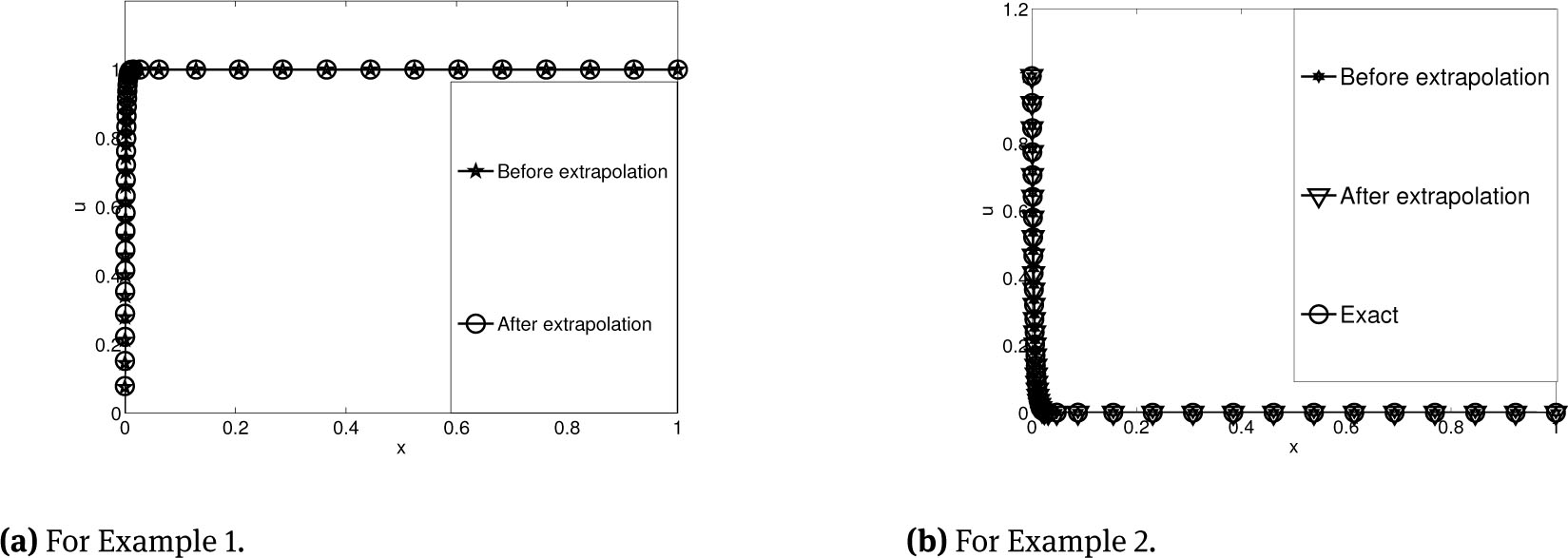
Numerical solution with N = 40 and ε = 2−8.

Error behaviour with N = 20 and ε = 10−2.
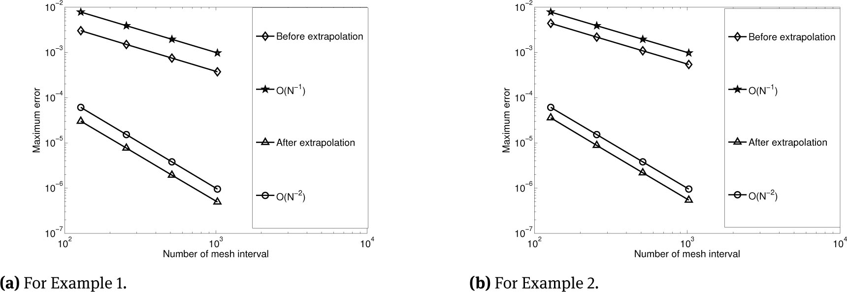
Loglog plot of maximum point-wise errors with ε = 10−8.
| ε | Number of intervals N | |||||||
|---|---|---|---|---|---|---|---|---|
| 16 | 32 | 64 | 128 | 256 | 512 | 1024 | ||
| 1e − 4 | before | 2.577e-2 | 1.238e-2 | 6.093e-3 | 3.020e-3 | 1.502e-3 | 7.503e-4 | 3.749e-4 |
| rate | 1.059 | 1.023 | 1.013 | 1.008 | 1.001 | 1.001 | ||
| after | 2.370e-3 | 5.182e-4 | 1.230e-4 | 2.998e-5 | 7.405e-6 | 1.974e-6 | 5.921e-7 | |
| rate | 2.193 | 2.075 | 2.037 | 2.018 | 1.908 | 1.737 | ||
| 1e − 8 | before | 2.796e-2 | 1.332e-2 | 6.188e-3 | 3.033e-3 | 1.504e-3 | 7.506e-4 | 3.742e-4 |
| rate | 1.069 | 1.106 | 1.029 | 1.012 | 1.003 | 1.004 | ||
| after | 2.776e-3 | 5.849e-4 | 1.269e-4 | 3.023e-5 | 7.678e-6 | 1.937e-6 | 4.947e-7 | |
| rate | 2.246 | 2.204 | 2.070 | 1.977 | 1.987 | 1.969 | ||
| N | S-mesh | B-S-mesh | Adaptive grid | |
|---|---|---|---|---|
| before | 1.488e-2 | 1.545e-2 | 1.859e-2 | |
| 32 | rate | 0.705 | 0.932 | 0.959 |
| after | 4.643e-4 | 3.850e-4 | 6.346e-4 | |
| rate | 1.403 | 1.769 | 1.998 | |
| before | 5.399e-3 | 4.141e-3 | 4.411e-3 | |
| 128 | rate | 0.794 | 0.983 | 1.014 |
| after | 6.154e-5 | 4.647e-5 | 3.590e-5 | |
| rate | 1.586 | 1.968 | 2.028 | |
| before | 1.759e-3 | 1.053e-3 | 1.087e-3 | |
| 512 | rate | 0.843 | 0.995 | 1.003 |
| after | 6.557e-6 | 4.181e-6 | 2.185e-6 | |
| rate | 1.686 | 1.986 | 2.007 | |
7 Concluding remarks
In this work, a higher order accurate method is used to compute the solution of a class of parameterized nonlinear singularly perturbed differential equation. First, we use the backward Euler difference scheme on the adaptive grid, then Richardson extrapolation technique is used on the computed solution. Clearly, after extrapolation the error of the numerical solution is considerably decreased. Theoretical estimates are supported with the help of numerical results. The advantage of the adaptive grid over Shishkin type meshes is evident from the theoretical estimates obtained as well as from the numerical results shown.
Acknowledgement
The authors express their sincere thanks to the anonymous referees for their valuable suggestions to improve the quality of the manuscript. The authors also express their sincere thanks to DST, Govt. of India for supporting this work under research grant no. SR/FTP/MS-027/2012 and for providing INSPIRE fellowship (IF 150650).
References
[1] Amiraliyev, G.M. and Duru, H. A note on parameterized singular perturbation problem. J. Comput. Appl. Math., 182:233–242 (2005).10.1016/j.cam.2004.11.047Search in Google Scholar
[2] Amiraliyeva, I.G. and Amiraliyev, G.M. Uniform difference method for a parameterized singularly perturbed delay differential equations. Numer. Alog., 52:509–521 (2009).10.1007/s11075-009-9295-ySearch in Google Scholar
[3] Cen, Z. A second-order difference scheme for a parameterized singular perturbation problem. J. Comput. Appl. Math., 221:174–182 (2008).10.1016/j.cam.2007.10.004Search in Google Scholar
[4] Chen, Y. Uniform convergence analysis of finite difference approximations for singularly perturbation problem on an adaptive grid. Adv. Comput. Math., 24:197–212 (2006).10.1007/s10444-004-7641-0Search in Google Scholar
[5] Das, P. and Srinivasan, N. Richardson extrapolation method for singularly perturbed convection-diffusion problems on adaptively generated mesh. Comput. Model. Eng. Sci., 90:463–485 (2013).Search in Google Scholar
[6] Das, P. Comparison of A priori and A posteriori Meshes for Singularly Perturbed Nonlinear Parameterized Problems. J. Comput. Appl. Math., 290:16–25 (2015).10.1016/j.cam.2015.04.034Search in Google Scholar
[7] Farrell, P.A., Hegarty, A.F., Miller, J.J.H., O’Riordan, E. and Shishkin, G.I. Robust Computational Techniques for Boundary Layers. Chapman & Hall/CRC Press, Boca Raton, FL (2000).10.1201/9781482285727Search in Google Scholar
[8] Jankowski, T. and Lakshmikantham, V. Monotone iterations for diffrential equation with parameter. J. Appl. Math. stoch. Anal., 10(3):273–278 (1997).10.1155/S1048953397000348Search in Google Scholar
[9] Kellogg, R.B. and Tsan, A. Analysis of some differences approximations for a singular perturbation problem without turning point. Math. Comp., 32: 1025–1039 (1978).10.1090/S0025-5718-1978-0483484-9Search in Google Scholar
[10] Kopteva, N. and Stynes, M. A robust adaptive method for a quasi-linear one dimensional convection-diffusion problem. SIAM J. Numer Anal., 39:1446–1467 (2001).10.1137/S003614290138471XSearch in Google Scholar
[11] Liu, X. and Mcare, F.A. A Monotone iterative methods for boundary value problems of parameteric differential equation. J. Appl. Math. stoch. Anal., 14(2):183–187 (2001).10.1155/S1048953301000132Search in Google Scholar
[12] Mackenzie, J. Uniform convergence analysis of an upwind finite differences approximation of a convection-diffusion boundary value problem on an adaptive grid. IMA J. Numer Anal., 19:233–249 (1999).10.1093/imanum/19.2.233Search in Google Scholar
[13] Miller, J.J.H., O’Riordan, E. and Shishkin, G.I. Fitted numerical methods for singular perturbation problems revised edition. World Scientific, Singapore (2012).10.1142/8410Search in Google Scholar
[14] Mohapatra, J. and Natesan, S. Unformaly convergent second-order numetical method for singularly perturbed delay differential equations. Neural Parallel Sci. Comput., 16:353–370 (2008).Search in Google Scholar
[15] Mohapatra, J. and Natesan, S. Parameter–uniform numerical method for global solution and global normalized flux of singularly perturbed boundary value problems using grid equidistribution. Comput. Math. Appl., 60:1924–1939 (2010).10.1016/j.camwa.2010.07.026Search in Google Scholar
[16] Natividad, M.C. and Stynes, M. Richardson extrapolation for a convection-diffusion problem using a Shishkin mesh. Appl. Numer. Math., 45:315–329 (2003).10.1016/S0168-9274(02)00212-XSearch in Google Scholar
[17] Pomentale, T. A constructive theorem of existence and uniqueness for problem y′ = f(x, y,λ), y(a) = α, y(b) = β. Z. Angrew. Math. Mech., 56(8):387–388 (1976).10.1002/zamm.19760560806Search in Google Scholar
[18] Ronto, M. and Csikos-Marinets, T. On the investigation of some non-linear boundary value problems with parameter. Math. Notes, Miscolc., 1:157–166 (2000).10.18514/MMN.2000.29Search in Google Scholar
[19] Roos, H.G., Stynes, M. and Tobiska, L. Numerical methods for singularly perturbed differential equations. Springer, Berlin (1996).10.1007/978-3-662-03206-0Search in Google Scholar
[20] Shakti, D. and Mohapatra, J. Layer-adapted meshes for parameterized singular perturbation problem. Procedia Engineering, 127:539–544, (2015).10.1016/j.proeng.2015.11.342Search in Google Scholar
[21] Turkyilmazoglu, M. Analytic approximate solutions of parameterized unperturbed and singularly perturbed boundary value problems. Appl. Math. Model., 35:3879–3886 (2011).10.1016/j.apm.2011.02.011Search in Google Scholar
[22] Vulanović, R., Herceg, D. and Petrović, N. On the extrapolation of a singulalrly perturbed boundary value problem. Computing, 36:69–79 (1986).10.1007/BF02238193Search in Google Scholar
[23] Xie, F., Wang, J., Zhang, W. and He, M. A novel method for a class of parameterized singularly perturbed boundary value problems. J. Comput. Appl. Math., 213:258–267 (2008).10.1016/j.cam.2007.01.014Search in Google Scholar
© 2017 Walter de Gruyter GmbH, Berlin/Boston
This article is distributed under the terms of the Creative Commons Attribution Non-Commercial License, which permits unrestricted non-commercial use, distribution, and reproduction in any medium, provided the original work is properly cited.
Articles in the same Issue
- Frontmatter
- Velocity and thermal slip effects on MHD third order blood flow in an irregular channel though a porous medium with homogeneous/ heterogeneous reactions
- Boundary Layer Flow and Heat Transfer of fluid particle suspension with nanoparticles over a nonlinear stretching sheet embedded in a porous medium
- Thermal Analysis of porous fin with uniform magnetic field using Adomian decomposition Sumudu transform method
- Two dimensional kinematic surfaces with constant scalar curvature in Lorentz-Minkowski 7-space
- Influence of nonlinear thermal radiation and viscous dissipation on three-dimensional flow of Jeffrey nano fluid over a stretching sheet in the presence of Joule heating
- A second order numerical method for a class of parameterized singular perturbation problems on adaptive grid
- The generalized fractional order of the Chebyshev functions on nonlinear boundary value problems in the semi-infinite domain
- Nonlinear Dynamics Analysis for the Taut Inclined Cable Excited by Deck Vibration