Analytical and numerical validation for solving the fractional Klein-Gordon equation using the fractional complex transform and variational iteration methods

1 Introduction

Fractional differential equations (FDEs) have recently been applied in various areas of engineering, science, finance, applied mathematics, bio-engineering and others [1]. Consequently, considerable attention has been given to the solutions of FDEs of physical interest. This kind of equations is more complex than ordinary differential equations. In the field of numerical treatment of this kind, a great attention has been recently dedicated to the development efficient and accurate numerical methods [2]. Among of these methods are, variational iteration method [3], homotopy perturbation method [4], Adomian decomposition method [5], homotopy analysis method [6] and collocation methods [7].

The Klein-Gordon equation plays a significant role in mathematical physics and many scientific applications, such as solid-state physics, nonlinear optics, and quantum field theory. The equation has attracted much attention in studying solitons ([8], [9]) and condensed matter physics, in investigating the interaction of solitons in a collisionless plasma, the recurrence of initial states, and in examining the nonlinear wave equations [10]. The study of numerical solutions of the Klein-Gordon equation has been investigated considerably in the last few years. For example, Wazwaz has obtained the various exact traveling wave solutions such as, compactions, solitons and periodic solutions by using the tanh method [11]. In the previous studies, the most papers have carried out different spatial discretization of the equation ([12], [13]). Where the numerical solution of this equation is given using, radial basis functions in [14], collocation and finite difference-collocation methods in [15], and the spline approach in [16]. Also, recently, an integral equation formalism in [17], the implicit RBF meshless approach [18] and the compact difference scheme [19] are given to solve numerically the FKGE. {The main aim of this paper is devoted to implement the fractional complex transform method to convert the nonlinear FKGE to an ODE and then use the VIM to solve the resulting problem.

We describe some necessary definitions and mathematical preliminaries of the fractional calculus theory which will be used further in this work.

2 Chain rule for fractional calculus

In previous papers ([22]-[24]), the authors used the following chain rule

to convert a fractional differential equation with Jumarie's modification of Riemann-Liouville derivative into its classical differential partner. In [25], the authors showed that this chain rule is invalid by giving a counter example as follows: Assume, s = t^α, 0 < α < 1 and u = s^m, i.e., u = t^mα, then

Now we calculate ∂u∂s∂αs∂tα.

Since ∂u∂s=msm−1=mtαm−α and

Then,

This shows that, ∂αu∂tα≠∂u∂s∂αs∂tα. In [25] the authors show that

where σ_t denotes the sigma index. These formula is called the modified chain rule. From the above example we can see that σt=Γ(1+mα)mΓ(1+mα−α). For more details, see [26].

3 Reducing the nonlinear FKGE to ordinary differential equation

In this section, to demonstrate the effectiveness of our approach, we will apply the complex transformation of Li and He to construct an approximate solution for the nonlinear fractional Klein-Gordon equation. Consider the following general form of FKGE

where Dtα denotes the fractional derivative of order α with respect to t, Dxβ denotes the fractional derivative of order β with respect to x, u(x, t) is unknown function, and a, b, c and γ are known constants with γ ∈ ℝ, γ ≠ ±1. We also assume the following initial conditions

and the following boundary conditions u(0, t) = u(1, t) = 0.

Li and He proposed a fractional complex transform for converting fractional differential equations into ordinary differential equations, so that all analytical methods for advanced calculus can be easily applied to fractional calculus ([23], [24]).

Now, we will reduce the given nonlinear fractional Klein-Gordon equation (3) to an ordinary differential equation in the following steps.

1. Take the following fractional complex transform:

   u(x,t)=U(ξ), ξ=Kt2αΓ(1+2α)+Lx2βΓ(1+2β),(5)

   where K and L are constants.

2. By using the fractional modified chain rule (2), we can obtain the following forms:

   Dt2αu=σtd2udξ2Dt2αξ,Dx2βu=σxd2udξ2Dx2βξ.(6)

3. With the help of formula (1), we find that:

   Dt2αt2α=Γ(1+2α),Dx2βx2β=Γ(1+2β).(7)

4. Use the equations (6) and (7) in Eq.(5) we can obtain:

   Dt2αu=σtKU″,Dx2βu=σxLU″,(8)

   where the prime denotes the derivative with respect to ξ.

5. Without loss of generality we can take σ_t = σ_x = ℓ where ℓ is a constant. So, Eq.(3) will convert to the following ordinary differential equation:

   (Kℓ+aLℓ)U″+bU+cUγ=0.

6. Rewrite the above ODE in the form:

   U″(ξ)+χ1U(ξ)+χ2Uγ(ξ)=0,(9)

   where χ1=b(Kℓ+aLℓ) and χ2=c(Kℓ+aLℓ).

4 Procedure of solution with VIM

In this section, we implement VIM for solving nonlinear ODE (9) with suitable boundary conditions. According to VIM, we construct the following recurrence formula

where λ is a general Lagrange multiplier. Making the above correction functional stationary

where δU~n, is considered as restricted variation, i.e., δU~n=0, yields the following stationary conditions (by comparison the two sides in the above equation)

Eqs.(11) are called Lagrange-Euler equation and its natural boundary conditions, the Lagrange multiplier, therefore

Now, by substituting from (12) in (10), the following variational iteration formula can be obtained

Now, we start with initial approximation

for some constants A = U(0) and B = U′(0). By using the above iteration formula (13), we can directly obtain the first components of the solution of (9) as follows

and so on. The unknown variables A and B are computed if we satisfy the boundary conditions.

5 Numerical simulation

In this section, we solve numerically the nonlinear fractional Klein-Gordon equation where we use the complex transformation method to reduce it as ODE, then we solve the resulting ODE using VIM. Some numerical examples are presented to validate the solution scheme [27]. To achieve this propose, we consider the following three cases.

Fig. 1

The behavior of the approximate solution using RK4 (Top) and VIM (Bottom) with different values of α and β.

Fig. 2

The behavior of the approximate solution using RK4 (Top) and VIM (Bottom) with different values of a, b and c.

Fig. 3

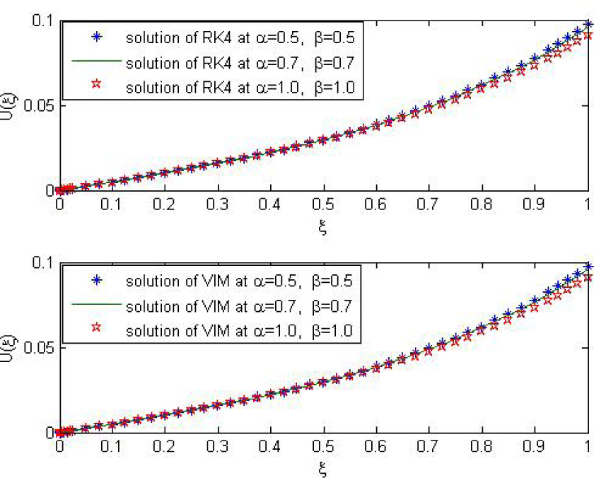
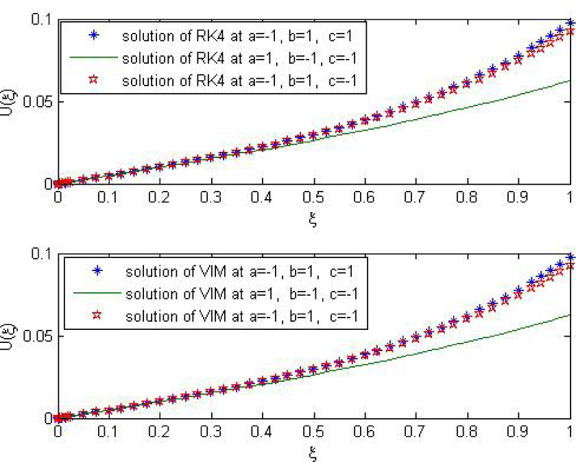
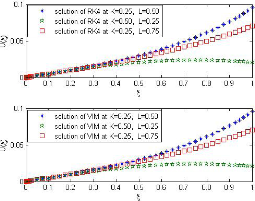
The behavior of the approximate solution using RK4 (Top) and VIM (Bottom) with different values of K and L.

6 Conclusion and remarks

In this article, the properties of the fractional complex transform method are used to reduce the nonlinear fractional Klein-Gordon equation to ordinary differential equation. The resulting ODE is solved by using variational iteration method. The obtained approximate solution using the suggested methods is in excellent agreement with the numerical solution using the forth order Runge-Kutta method and show that these approaches can be solved the problem effectively and illustrates the validity and the great potential of the proposed technique. All computation in this paper are done using Matlab 8.0.

References

[1] I. Podlubny, Fractional Differential Equations, Academic Press, New York, 1999.Search in Google Scholar
[2] N. H. Sweilam, M. M. Khader and A. M. Nagy, Numerical solution of two-sided space-fractional wave equation using finite difference method, J. of Computional and Applied Mathematics, 235, p.(2832-2841), 2011.10.1016/j.cam.2010.12.002Search in Google Scholar
[3] J. H. He, Approximate analytical solution for seepage flow with fractional derivatives in porous media, Computer Methods in Applied Mechanics and Engineering, 167(1-2), p.(57-68), 1998.10.1016/S0045-7825(98)00108-XSearch in Google Scholar
[4] A. M. A. El-Sayed, A. Elsaid and D. Hammad, A reliable treatment of homotopy perturbation method for solving the nonlinear Klein-Gordon equation of arbitrary (fractional) orders, Journal of Applied Mathematics, 2012, p.(1-13), 2012.10.1155/2012/581481Search in Google Scholar
[5] M. M. Khader, A new formula for Adomian polynomials and the analysis of its truncated series solution for the fractional non-differentiable IVPs, ANZIAM J., 55, p.(69-92), 2014.10.1017/S1446181113000321Search in Google Scholar
[6] I. Hashim, O. Abdulaziz and S. Momani, Homotopy analysis method for fractional IVPs, Commun. Nonlinear Sci. Numer. Simul., 14, p.(674-684), 2009.10.1016/j.cnsns.2007.09.014Search in Google Scholar
[7] M. M. Khader, The use of generalized Laguerre polynomials in spectral methods for fractional-order delay differential equations, J. of Computational and Nonlinear Dynamics, 8, p.(041018:1-5), 2013.10.1115/1.4024852Search in Google Scholar
[8] R. Sassaman and A. Biswas, Soliton solutions of the generalized Klein-Gordon equation by semi-inverse variational principle, Mathematics in Engineering Science and Aerospace, 2(1), p.(99-104), 2011.Search in Google Scholar
[9] R. Sassaman and A. Biswas, 1-soliton solution of the perturbed Klein-Gordon equation, Physics Express, 1(1), p.(9-14), 2011.Search in Google Scholar
[10] S. M. El-Sayed, The decomposition method for studying the Klein-Gordon equation, Chaos, Solitons and Fractals, 18(5), p.(1026-1030), 2003.10.1016/S0960-0779(02)00647-1Search in Google Scholar
[11] A. M. Wazwaz, Compacton solitons and periodic solutions for some forms of nonlinear Klein-Gordon equations, Chaos, Solitons and Fractals, 28(4), p.(1005-1013), 2006.10.1016/j.chaos.2005.08.145Search in Google Scholar
[12] A. K. Golmankhaneh and D. Baleanu, On nonlinear fractional Klein-Gordon equation, Signal Processing, 91, p.(446-451), 2011.10.1016/j.sigpro.2010.04.016Search in Google Scholar
[13] E. Yusufoglu, The variational iteration method for studying the Klein-Gordon equation, Applied Mathematics Letters, 21(7), p.(669-674), 2008.10.1016/j.aml.2007.07.023Search in Google Scholar
[14] M. Dehghan and A. Shokri, Numerical solution of the nonlinear Klein-Gordon equation using radial basis functions, Journal of Computational and Applied Mathematics, 230, p.(400-410), 2009.10.1016/j.cam.2008.12.011Search in Google Scholar
[15] M. Lakestani and M. Dehghan, Collocation and finite difference-collocation methods for the solution of nonlinear Klein-Gordon equation, Computer Physics Commun., 181, p.(1392-1401), 2010.10.1016/j.cpc.2010.04.006Search in Google Scholar
[16] J. Rashidini and R. Mohammadi, Tension spline approach for the numerical solution of nonlinear Klein-Gordon equation, Computer Physics Communications, 181, p.(78-91), 2010.10.1016/j.cpc.2009.09.001Search in Google Scholar
[17] T. S. Jang, An integral equation formalism for solving the nonlinear Klein-Gordon equation, Appl. Math. Comput. 243, p.(322-338), 2014.10.1016/j.amc.2014.06.004Search in Google Scholar
[18] M. Dehghan, M. Abbaszadeh and A. Mohebbi, An implicit RBF meshless approach for solving the time fractional nonlinear sine-Gordon and Klein-Gordon equations, Eng. Anal. Bound Elem. 50, p.(412-434) 2015.10.1016/j.enganabound.2014.09.008Search in Google Scholar
[19] S. Vong and Z. Wang, A compact difference scheme for a two dimensional fractional Klein-Gordon equation with Neumann boundary conditions, J. Comput. Phy., 274, p.(268-282), 2014.10.1016/j.jcp.2014.06.022Search in Google Scholar
[20] M. M. Khader, On the numerical solutions for the fractional diffusion equation, Communications in Nonlinear Science and Numerical Simulations, 16, p.(2535-2542), 2011.10.1016/j.cnsns.2010.09.007Search in Google Scholar
[21] K. B. Oldham and J. Spanier, The Fractional Calculus, Academic Press, New York, 1974.Search in Google Scholar
[22] R. W. Ibrahim, Fractional complex transforms for fractional differential equations, Advan. in Diff. Equat., 2012 192, 2012, doi:10.1186/1687-1847-2012-192.Search in Google Scholar
[23] Z. B. Li and J. H. He, Fractional complex transformation for fractional differential equations, Math. Comput. Appl., 15, p.(970-973), 2010.10.3390/mca15050970Search in Google Scholar
[24] Z. B. Li and J. H. He, Application of the fractional complex transform to fractional differential equations, Nonlinear Sci. Lett. A, 2(3), p.(121-126), 2011.Search in Google Scholar
[25] J. H. He, S. K. Elagan and Z. B. Li, Geometrical explanation of the fractional complex transform and derivative chain rule for fractional calculus, Phys. Lett. A, 376, p.(257-259), 2012.10.1016/j.physleta.2011.11.030Search in Google Scholar
[26] M. Saad, S. K. Elagan, Y. S. Hamed and M. Sayed, Using a complex transformation to get an exact solution for fractional generalized coupled MKDV and KDV equations, International Journal of Basic & Applied Sciences 13(1), p.(23-25), 2013.Search in Google Scholar
[27] M. M. Khader, An efficient approximate method for solving linear fractional Klein-Gordon equation based on the generalized Laguerre polynomials, International Journal of Computer Mathematics, 90(9), p.(1853-1864), 2013.10.1080/00207160.2013.764994Search in Google Scholar
© 2016 Walter de Gruyter GmbH, Berlin/Boston
This article is distributed under the terms of the Creative Commons Attribution Non-Commercial License, which permits unrestricted non-commercial use, distribution, and reproduction in any medium, provided the original work is properly cited.
Articles in the same Issue
- Frontmatter
- Original Articles
- Dynamic Analysis of Coupled Vehicle-Bridge System with Uniformly Variable Speed
- Research Article
- A note on soliton solutions of Klein-Gordon-Zakharov equation by variational approach