Homotopy analysis transform algorithm to solve time-fractional foam drainage equation

1 Introduction

In the past few decades, developments of the fractional derivative and fractional differential equations are the emerging tools in the field of fractional calculus [1, 2]. Fractional differential equations (FDEs) have been the focus of many studies due to their frequent appearances in various applications in fluid mechanics, viscoelasticity, biology, physics, electrical network, control theory of dynamical systems, chemical physics, optics and signal processing, as they can be modeled by linear and non-linear fractional order differential equations [3-5].

In the open literature there exist no methods that produce an exact solution fractional differential equations, especially it is hard to obtained for nonlinear equations. Only approximate solutions can be derived using linearization or successive or perturbation methods. Some of these are Adomian’s decomposition method [6], variation iteration method [7], homotopy perturbation method [8], homotopy analysis method [9, 10], homotopy asymptotic method [11] and differential transform method [12].

In recent years, many authors have paid attention to studying the solutions of linear and nonlinear partial differential equations by using various methods combined with the Laplace transform. These include the Laplace decomposition methods [13], the homotopy perturbation transform method [14] and the homotopy analysis transform method [15, 16].

The aim of this paper is to apply for the first time the homotopy analysis transform method to study the solution of time-foam drainage model described by [17]

subject to the initial condition:

It is a simple model of the flow of liquid through channels (Plateau borders) and nodes (intersection of four channels) between the bubbles, driven by gravity and capillarity [18]. Previously the Eq. (1) have been studied by different researcher using the methods like Adomian’s decomposition method [19] and homotopy analysis method \cite{amr}. But as far the possible information of the authors this is the first attempted for finding the approximate analytical solution of Eq. (1) by using MHATM method.

Rest of the paper organized as follows: paper stated with introduction and some basic needful definition. Basic idea of modified homotopy analysis transforms method is presented in section 2. Application and numerical discussion of the MHATM method for approximate solution of time-fractional foam drainage model is given in section 3. Finally, conclusions are drawn in section 4.

2 Basic idea of modified homotopy analysis transforms method

To demonstrate the elementary idea of the MHATM for the fractional partial differential equation, we consider the following general fractional partial differential equation:

where R[x] is a linear operator in x, N[x] is a nonlinear operator in x, g(x, t) is a continuous function. For simplicity, we ignore all boundary or initial conditions, which can be treated in the similar way. Now the methodology consists of applying Laplace transform first on both sides of Eq. (2.1), we get

Now, using the differentiation property of the Laplace transform, we have

We define the nonlinear operator

where q ∈ [0, 1] be an embedding parameter and ϕ(x, t; q) is the real function of x, t and q. By means of generalizing the traditional homotopy analysis methods [21, 22], construct the zero order deformation equation

where ħ is a nonzero auxiliary parameter which helps us to increase the convergence results, H(x, t) an auxiliary function, u₀(x, t) is an initial guess of u(x, t) and ϕ(x, t; q) is an unknown function. It is important that one has great freedom to choose auxiliary parameters in MHATM. This freedom plays an important role in establishing the keystone of validity and flexibility of MHATM. Obviously, when q = 0 and q = 1, it holds

respectively. Thus, as q increases from 0 and 1, the solution varies from the initial guess u₀(x, t) to the solution u(x, t). Expanding ϕ(x, t; q) in Taylor’s series with respect to q, we have

where um(x,t)=1m!∂mϕ(x,t;q)∂qm|q=0.

For the sake of convenience, the expression in nonlinear operator form has been modified in homotopy analysis transforms method i,e the nonlinear term N[x, t]u(x, t) is expanded in terms of homotopy polynomials [23] as

If the auxiliary linear operator, the initial guess, the auxiliary parameter ħ and the auxiliary function are properly chosen, the series (2.6) converges at q = 1, we have

which must be one of the solutions of original nonlinear equations. Defines the vectors

Differentiating equation (2.5)m time with respect to embedding parameter q and then setting q = 0 and finally dividing them by m!, we obtain the m−th order deformation equation

Operating the inverse Laplace transform on both sides, we get

where

and ξm={0,m≤1,1 m>1.

In this way, it is easy to obtain u_m(x, t) for m ≥ 1, at M−th order, we have

when M → ∞, we get an accurate approximation of the original equation (2.1).

The novelty of our proposed algorithm is that a new correction functional in the nonlinear term as a series of homotopy polynomials in the u_m(x, t). We combine the new hybrid iterative algorithm for nonlinear fractional partial differential equations arising in science and engineering.

3 Application of MHATM and numerical discussions

For the application of MHATM, we have consider time-fractional foam drainage model as follows:

subject to the initial condition:

For α = 1, the exact solutions of Eq. (3.1) is given by [17],

Applying the Laplace transform on both sides in Eq. (3.1) and after using the differentiation property of Laplace transform for fractional derivative, we get

We choose the linear operator as

with property 𝓛[c] = 0, where c is a constant. We now define a nonlinear operator as

Using the above definition, with assumption H(x, t) = 1, we construct the so-called zeroth-order deformation equation

Obviously, when q = 0 and q = 1

Thus, we obtain the m−th order deformation equation

Operating the inverse Laplace transform on both sides in Eq. (3.7), we get

where

Now the solution of m−th order deformation equations (3.7) is

Where Pm1,  Pm2 and Pm3 are homotopy polynomials given by

where ϕ(x, t; q) is given by

Finally, we have

Using the initial approximation u0(x,t)=u(x,0)=−c  tanh(c  x) and the iterative scheme (3.10), we obtain the various iterates

Proceeding in this manner, the rest of the components u_m(x, t) for m ≥ 3 can be completely obtained and the series solutions are thus entirely determined.

Hence, the solution of equation (3.1) is given as

3.1 Numerical discussion

In this section, we discussed the obtained results from the previous section through different graphical representations. Figure 1 represents comparisons of the 4th order approximate solution of the function u(x, t) for different values of the fractional derivative α with the known exact solution. It can be noted that there exist a very good agreement between them.

Fig. 1

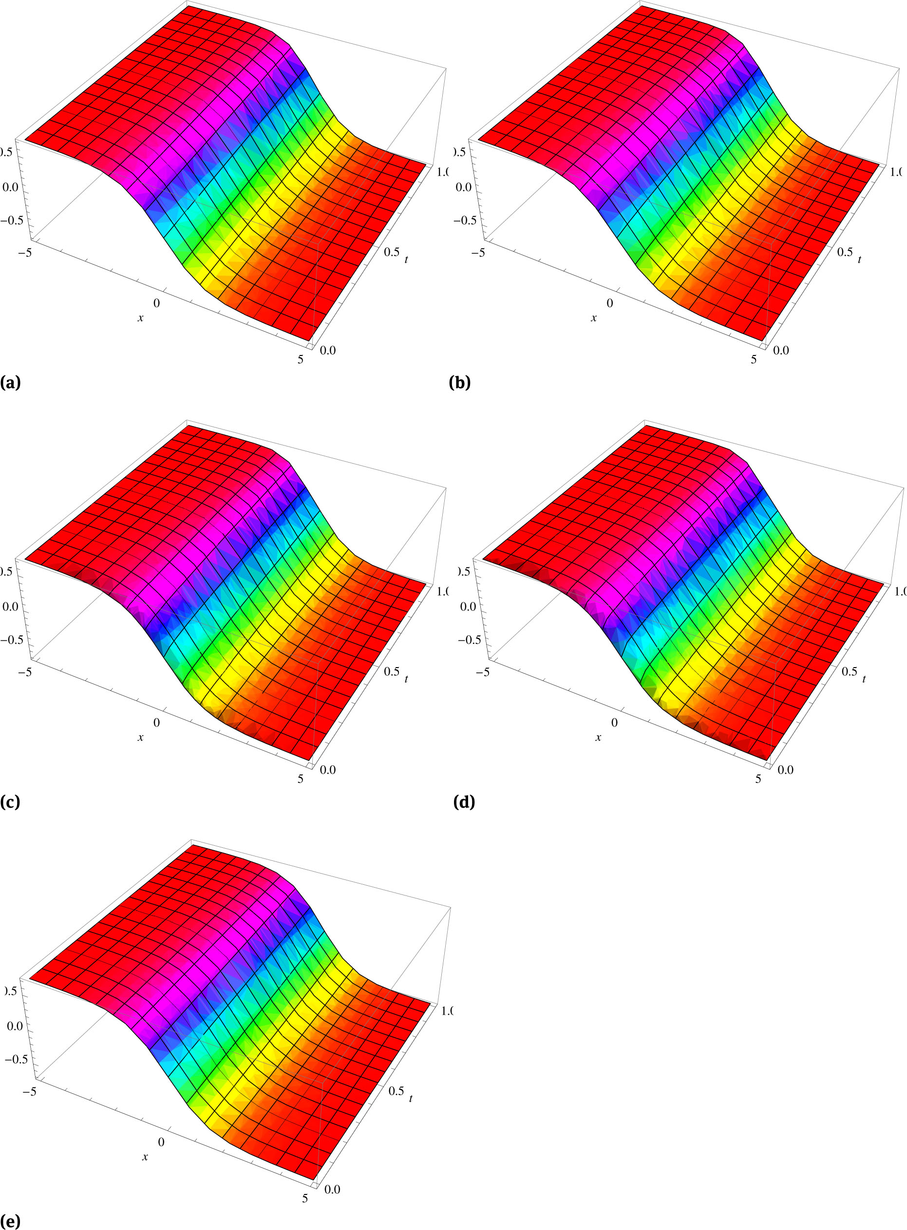
The 4th order approximate solution of the Foam model: (a) u₄(x, t) when α = 1. (b) u₄(x, t) when α = 0.75. (c) u₄(x, t) when α = 0.5. (d) u₄(x, t) when α = 0.25. (e) Exact solution u(x, t) when α = 1.

To validate the efficiency and accuracy of the analytical scheme, we give the absolute error curve E4 = |u(x, t) − u₄(x, t)|. Figure 2 shows that our solution obtained by proposed methods converges very rapidly to the exact solutions in only 4th order approximations.

Fig. 2

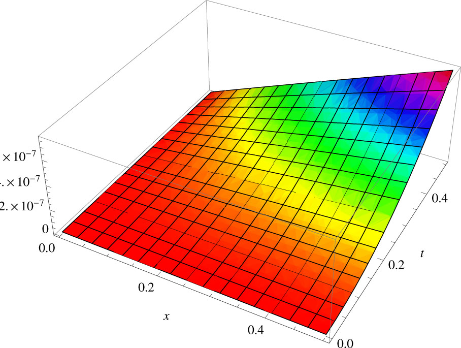
Plot of absolute error E₄ = |u(x, t) − u₄(x, t)|.

The behavior of the approximate analytical solution of Eq. (3.1) obtained by the MHATM for different fractional Brownian motions α = 0.7, α = 0.8, α = 0.9 and standard motions, i.e. α = 1 is shown in fig. 3. It is seen from fig. 3 that the solution obtained by MHATM method increases very rapidly with the increases in t at the value of x = 1.

Fig. 3

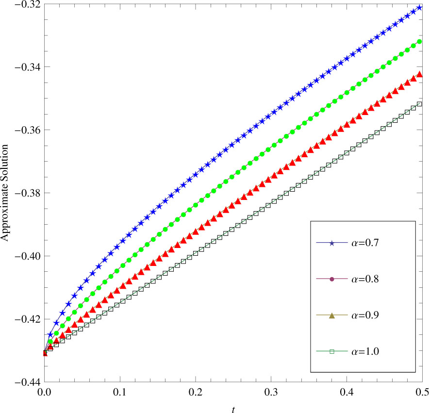
Plot of u₄(x, t) vs. time t at x = 1 and different value of α.

Table 1

The absolute error in the solution of time fractional STO equation using MHATM at different points of xand twhen α= 1.

(x, t)	|uexact − uMHATM|
(0.1,0.1)	6.17055 × 10−5
(0.1,0.2)	2.44401 × 10−4
(0.1,0.3)	5.42701 × 10−4
(0.2,0.1)	1.20503 × 10−4
(0.2,0.2)	4.75281 × 10−4
(0.2,0.3)	1.05033 × 10−3
(0.3,0.1)	1.74288 × 10−4
(0.3,0.2)	6.85009 × 10−4
(0.3,0.3)	1.50823 × 10−3

Table 2

L₂ and L₁ error norm in case of STO equation using MHATM at various points of xwhen α= 1.

X	L2 norm for u(x, t)	L∞ norm for u(x, t)
0.1	2.82936 × 10−4	5.42701 × 10−4
0.2	5.48705 × 104	1.05033 × 10−3
0.3	7.89176 × 10−4	1.50823 × 10−3

4 Conclusions

In this paper we have successfully applied MHATM for finding the approximate analytical solution of a timefractional foam drainage model. The main output of this work is the nonlinear operator has been modified in homotopy analysis transforms method i,e the nonlinear term N[x, t]u(x, t) is expanded in terms of homotopy polynomials, as a result we get a rapid convergence of the series solution. To validate the obtained result different types of graphs are presented. The above procedure shows that the MHATM method is efficient and powerful in solving wide classes of equations in particular evolution fractional order equations like foam drainage model. It, therefore, provides more realistic series solutions that generally converge very rapidly in real physical problems.

References

[1] K. S. Miller, B. Ross, An Introduction to the Fractional Calculus and Fractional Differential Equations, Wiley, New York 1993.Search in Google Scholar
[2] K. B. Oldham, J. Spanier, The Fractional Calculus: Integrations and differentiations of arbitrary order, Academic Press, New York 1974.Search in Google Scholar
[3] I. Podlubny, Fractional differential equations, Academic Press, San Diego, New York 1999.Search in Google Scholar
[4] K. Diethelm, An algorithm for the numerical solution of differential equations of fractional order, Electron. Trans. Numer. Anal., 5 (1997) 1–6.Search in Google Scholar
[5] K. Diethelm, N.J. Ford, Analysis of fractional differential equations, J. Math. Anal. Appl., 265 (2002) 229–248.10.1007/978-3-642-14574-2Search in Google Scholar
[6] D.J. Evans, H. Bulut, A new approach to the gas dynamics equation: an application of the decomposition method, Inter. J. Comput. Math., 79 (7) (2002) 817–822.10.1080/00207160211297Search in Google Scholar
[7] M. G. Sakar, F. Erdogan, A. Yildirim, Variational iteration method for the time-fractional Fornberg – Whitham equation, Comput. Math. Appl., 63 (2012) 1382–1388.10.1016/j.camwa.2012.01.031Search in Google Scholar
[8] P. K. Gupta, M. Singh, Homotopy perturbation method fractional Fornberg–Whitham equation, Comput. Math. Appl., 61 (2011) 250–254.10.1016/j.camwa.2010.10.045Search in Google Scholar
[9] S. J. Liao, On the homotopy analysis method for nonlinear problems, Appl. Math. Comput., 147 (2004) 499–513.10.1016/S0096-3003(02)00790-7Search in Google Scholar
[10] K. Vishal, S. Kumar, S. Das, Application of homotopy analysis method for fractional swift Hohenberg equation-revisited, Appl. Math. Modell., 36 (8) (2012) 3630–3637.10.1016/j.apm.2011.10.001Search in Google Scholar
[11] R.K. Pandey, O.P. Singh, V.K. Baranwal, An analytic algorithm for the space-time fractional advection-dispersion equation, Comput. Phys. Commun., 182 (2011) 1134–1144.10.1016/j.cpc.2011.01.015Search in Google Scholar
[12] V.K.Srivastava, M.K. Awasthi, S. Kumar, Analytical approximations of two and three dimensional time-fractional telegraphic equation by reduced differential transform method, Egypt J. Bas. Appl. Sci., 1 (2014) 60–66.10.1016/j.ejbas.2014.01.002Search in Google Scholar
[13] A.M. Wazwaz, The combined Laplace transform-Adomian decomposition method for handling nonlinear Volterra integrodifferential equations, Appl. Math. Comput., 216 (4) (2010) 1304–1309.10.1016/j.amc.2010.02.023Search in Google Scholar
[14] S. Kumar, A numerical study for solution of time fractional nonlinear shallow water equation in oceans, Z. Naturforschung 68 a (2013) 1–7.10.5560/zna.2013-0036Search in Google Scholar
[15] S. Kumar, M.M. Rashidi, New analytical method for gas dynamic equation arising in shock fronts, Comput. Phys. Commun., 185 (2014) 1947–1954.10.1016/j.cpc.2014.03.025Search in Google Scholar
[16] S. Kumar, A new analytical modelling for telegraph equation via Laplace transform, Appl. Math. Modell., 38 (2014) 3154– 3163.10.1016/j.apm.2013.11.035Search in Google Scholar
[17] G. Verbist, D. Weuire, A.M. Kraynik, The foam drainage equation, J. Phys. Condens. Matter 8 (1996) 3715–3731.10.1088/0953-8984/8/21/002Search in Google Scholar
[18] D. Weaire, S. Hutzler, S. Cox, M.D. Alonso, D. Drenckhan, The fluid dynamics of foams, J. Phys. Condens. Matter 15(2003) S65– S73.10.1088/0953-8984/15/1/307Search in Google Scholar
[19] Z. Dahmani, M.M. Mesmoudi, R. Bebbouch, The Foam Drainage equation with time- and space-fractional derivatives solved by the Adomian method, Electron. J. Qual. Theory Differ. Equ., 30 (2008) 1–10.10.14232/ejqtde.2008.1.30Search in Google Scholar
[20] H.H. Fadravi, H.S. Nik, R. Buzhabadi, Homotopy analysis method for solving Foam Drainage equation with space- and time-fractional derivatives, Int. J. Differ. Equ., (2011) (Article ID 237045).10.1155/2011/237045Search in Google Scholar
[21] S.J. Liao, The proposed homotopy analysis technique for the solution of nonlinear problems, Ph.D thesis, Shanghai Jiao Tong Univ. (1992)Search in Google Scholar
[22] S.J. Liao, Homotopy analysis method: A new analytical technique for nonlinear problems, Commun. Nonlinear Sci. Numer. Simul., 2 (1997) 95–100.10.1016/S1007-5704(97)90047-2Search in Google Scholar
[23] Z. Odibat, A.S. Bataineh, An adaptation of homotopy analysis method for reliable treatment of strongly nonlinear problems: construction of homotopy polynomials, Math. Meth. Appl. Sci., 38(5) (2015) 991–1000.10.1002/mma.3136Search in Google Scholar
© 2016 Walter de Gruyter GmbH, Berlin/Boston
This article is distributed under the terms of the Creative Commons Attribution Non-Commercial License, which permits unrestricted non-commercial use, distribution, and reproduction in any medium, provided the original work is properly cited.
Articles in the same Issue
- Frontmatter
- Original Articles
- Dynamic Analysis of Coupled Vehicle-Bridge System with Uniformly Variable Speed
- Research Article
- A note on soliton solutions of Klein-Gordon-Zakharov equation by variational approach
- Analytical and numerical validation for solving the fractional Klein-Gordon equation using the fractional complex transform and variational iteration methods
- Thermal radiation and chemical reaction effects on boundary layer slip flow and melting heat transfer of nanofluid induced by a nonlinear stretching sheet