New Insights on the Multivariate Skew Exponential Power Distribution

Jorge M. Arevalillo; Hilario Navarro

doi:10.1515/ms-2023-0039

Article Open Access

New Insights on the Multivariate Skew Exponential Power Distribution

Jorge M. Arevalillo and Hilario Navarro

Published/Copyright: March 31, 2023

Published by

Become an author with De Gruyter Brill

Author Information Explore this Subject

From the journal Mathematica Slovaca Volume 73 Issue 2

ABSTRACT

The multivariate exponential power is a useful distribution for modeling departures from normality in data by means of a tail weight scalar parameter that regulates the non-normality of the model. The incorporation of a shape asymmetry vector into the model serves to account for potential asymmetries and gives rise to the multivariate skew exponential power distribution. This work is aimed at revisiting the skew exponential power distribution taking as a starting point its formulation as a scale mixture of skew-normal distributions. The paper provides some highlights and theoretical insights on the role played by its parameters to assess two complementary aspects of the multivariate non-normality such as directional asymmetry and tail weight behavior regardless of the asymmetry. The intuition behind both issues relies on well-known mathematical ideas about skewness maximization and convex transform stochastic orderings.

2020 Mathematics Subject Classification: Primary 62H99; 60E15; Secondary 60E99

Keywords: Skew exponential power; asymmetry; skewness; tail weight; kurtosis

1. Introduction

The exponential power (EP) distribution has an ancient history in statistics which dates back to Subbotin’s pioneer work [42] with an early multivariate generalization introduced by De Simoni [41], later on quoted by the follow-up [24]; it can also be considered as a particular case of the Kotz-type family of distributions [31] as highlighted in [19: Section 3.2]. Unlike other non-normal distributions, like for example the t distribution, the EP family has the advantage of including distributions having heavier and lighter tails than the normal one with the normal model being an intermediate distribution within the family. Due to its flexibility and wide scope, a lot of research has been carried out since the aforementioned foundational works with contributions that show its usefulness both in univariate [1, 13, 14, 18, 25, 39, 45, 46] and multivariate settings [20, 22, 23, 32, 35], a matrix generalization of the model [40], its study in the context of the general class of elliptically contoured distributions [3, 21, 30, 38], some caveats about its limitation to remain closed under marginalization [27], as well as related variants to assess asymmetry [2, 6, 12] and some other models under which this family can be considered [37, 38].

This paper adopts the approach of several of the aforementioned works [19, 21, 24, 27] to define the multivariate EP distribution as follows: we say that an input vector X follows a p-dimensional exponential power distribution with location vector ξ and full rank scale matrix Ω if its probability density function (pdf) is given by

1.1 f(x;ξ,Ω,β)=βΓ(p2)πP/2Γ(P2β)2p/2β| Ω|−1/2exp{ −12[ (x−ξ)┬Ω−1(x−ξ) ]β },

x∈ℝp, where β > 0 is a tail weight parameter accounting for the peakedness of the model. The notation X ~ EP_p(ξ, Ω, β) is used to indicate that X has a distribution with pdf in (1.1). Note that when β = 1 the EP vector has a multivariate normal distribution N_p(ξ, Ω). Figure 1 illustrates the differences of peakedness by visual comparison of the shapes of the bidimensional normal (β = 1) and double exponential (β = 1/2) density functions.

Figure 1.

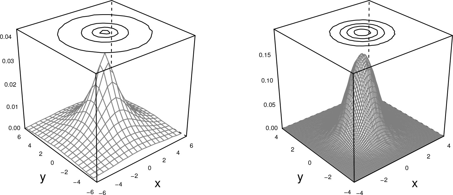
Probability density functions for the bivariate double exponential (left) and normal (right) variables with location ξ = (0,0) and scale matrix Ω = I₂.

The skew exponential power (SEP) class arises when asymmetry is injected into a EP distribution so that a skewed model is obtained as a result; some past works have addressed the issue dealing with different variants of skewed EP distributions: see the works [2, 6, 12] or the alternative formulation as a scale mixture of skew-normal (SMSN) distributions [15: Section 3]. This paper examines the multivariate SEP family from the latter representation, from which analytical closed expressions for moments can be obtained [16, 28], a relevant issue when addressing skewness maximization. The paper is organized as follows: The next section gives some background about the multivariate SN distribution and the SMSN representation of the SEP vector. Section 3 discusses the role played by the shape vector and the tail weight β as parameters that account for the multivariate non-normality of the model; some novel insights regarding the assessment of directional asymmetry, through the direction that yields the maximal skewness projection, as well as the connection of the tail weight parameter with well established multivariate convex transform stochastic orderings, are studied in order to enhance their interpretation in the assessment of the multivariate non-normality. Finally, Section 4 recaps the main findings of the paper suggesting yet unexplored ideas to advance progress towards future research directions.

2. The multivariate skew exponential power distribution

This section deals with some material aimed at presenting the SMSN formulation of the SEP distribution. Firstly, some background about the SN distribution and its extension to the SMSN family is provided; then the representation of the multivariate exponential power distribution as a scale mixture of normal (SMN) distributions is used in order to introduce the SMSN representation of the SEP model in a natural way.

2.1. The multivariate skew-normal and SMSN families

The multivariate skew-normal (SN) distribution was introduced by [9] to regulate asymmetry departures from normality. Here, it is adopted the notation of the original seminal works [8, 9] to define the pdf of a p-dimensional SN vector with location vector ξ = (ξ₁, …, ξ_p)^┬ and scale matrix Ω as follows:

2.1 f(x;ξ,α, Ω)=2ϕP(x−ξ;Ω)Φ(α┬ω−1(x−ξ)),x∈ℝp,

where ϕ_p(·; Ω ) denotes the pdf of a p-dimensional normal variate with zero mean and covariance matrix Ω, Φ is the distribution function of a standard N(0, 1) scalar variable, ω = diag(ω₁, …, ω_p) is a scale diagonal matrix with non negative entries such that Ω¯=ω−1Ωω−1 is a correlation matrix and α is a p-dimensional shape vector that regulates the asymmetry of the model. If α = 0, then the pdf in (2.1) reduces to the density of a normal vector with mean vector ξ and covariance matrix Ω. We use the notation X ~ SN_p(ξ, Ω, α) to indicate that X follows a p-dimensional skew-normal distribution with pdf given by (2.1).

Note that the diagonal matrix ω can be written as ω = (Ω ☉ I_p)^1/2, where the symbol ☉ denotes the entry-wise matrix product. It also holds that X = ξ + ωZ, where Z is a normalized multivariate skew-normal variable with pdf given by

2.2 f(z;0, α,Ω¯)=2ϕP(z;Ω¯)Φ(α┬z).

The normalized SN variate has a simple pdf and a tractable stochastic representation which enables its extension to the wider SMSN family in a natural way [11, 16, 17] (with reference [17] a posthumous reprint of [16]). This paper adopts the formulation from the aforementioned works to define a SMSN vector as follows:

Definition 1.

Let Z be a random vector such that Z~SNp(0,Ω¯,α), with pdf (2.2), and let S be a non negative scalar variable independent of Z. The random vector X = ξ + ωSZ, where ω is a diagonal matrix with non negative entries, is said to follow a multivariate SMSN distribution.

We put X ~ SMSN_p(ξ, Ω, α, H) with H the distribution function of the mixing variable S and Ω=ωΩ¯ω, to indicate that X follows a p-dimensiontal SMSN distribution. Note that when H is degenerate at S = 1, then X becomes a SN_p(ξ, Ω, α) vector.

2.2. The SMSN formulation of the skew exponential power distribution

The SMSN distribution reduces to a scale mixture of normal distributions when the shape vector is equal to the p-dimensional zero vector, a = 0_p, since the vector Z from Definition 1 has a p-dimensional normal distribution, i.e. Z~Np(0,Ω¯). We put X ~ SMN_p(ξ, Ω, H) to indicate that X follows a SMN distribution. The multivariate EP distribution with pdf (1.1) admits a SMN formulation as long as the tail weight parameter satisfies that 0 < β ≤ 1, as the following proposition shows [23].

Proposition 2.1

Let X be a p-dimensional vector such that X ~ EP_p(ξ, Ω, β). Then it holds that X ~ SMN_p(ξ, Ω, H) if and only if 0 < β ≤1. When β ϵ(0, 1) the distribution H of the mixing variable is absolutely continuous and it has pdf given by

2.3 hβ(s)=2P2(1−1β)Γ(1+P2)Γ(1+P2β)sp−3Sβ(12s−2;2−1β),s>0,

where Sβ(⋅;2−1β) denotes the pdf of a non-negative stable distribution having characteristic function φ(t)=exp{ −12|t|βe−iπ2β sign (t) }. On the other hand, when β = 1, H is the degenerate distribution at S = 1.

The result of Proposition 2.1 motivates to define the skew EP distribution as follows.

Definition 2.

Let Z be a vector such that Z~SNp(0,Ω¯,α) with pdf (2.2) and let S be a non negative scalar variable, independent of Z, with the density function of Proposition 2.1 for any β ϵ (0,1]. If ω is a diagonal matrix with non-negative entries, then we say that the random vector X = ξ + ωSZ follows a multivariate skew exponential power distribution.

We write X ~ SEP_p(ξ, Ω, α, β) to indicate that X follows a p-dimensional SEP distribution with location ξ, scale matrix Ω=ωΩ¯ω, shape vector α and tail weight parameter β ϵ (0,1]. It is worthwhile noting that the SEP family of distributions belongs to the wider skew-elliptical class of distributions [15] and it is also closed under full-rank affine transformations.

From the stochastic representation of the SEP vector in Definition 2, the mean vector and the covariance matrix of the model are obtained by combining (6.18) of [11] with Lemma 2.1:

Lemma 2.1.

Let X be a vector such that X ~ SEP_p(ξ, Ω, α, β). Then the moments of the mixing variable are given by E(Sk)=2k/2βΓ(p2)Γ(p+k2β)2k/2Γ(p2β)Γ(p+k2).

Proof. See the appendix. □

Then it can be shown in an easy way that

E(X)=ξ+E(S)2πγandvar(X)=E(S)2Ω−Ε(S)22πγγ′

with

E(S)=21−β2βΓ(p2)Γ(p+12β)Γ(p2β)Γ(p+12),E(S2)=21−ββ2Γ(p+22β)pΓ(p2β),γ=Ωη1+η′Ωηandη=ω−1α.

The stochastic representation also provides a natural strategy for the simulation of observations from a p-dimensional SEP vector. Although the observations from the SN vector ωZ can be obtained in an easy way using the functionalities of the sn R package [7], the non tractability of the density function (2.3) makes the simulation of the mixing variable a difficult task. However, for some specific tail weight parameters the mixing variable has a well-known distribution; in such cases we can simulate observations from S: for example, when β = 1, the model becomes the SN distribution, whereas β = 1/2 corresponds to the skewed version of the multivariate double exponential distribution, with the mixing variable S following a generalized gamma distribution [23]. Figure 2 displays the plots of the pdf for the skewed bivariate double exponential; it illustrates the effect caused by the parametric vector α on the shape of the densities as well as the contoured plots obtained after injection of asymmetry across different directions.

Figure 2.

Density functions of the bivariate double exponential (β = 1/2), with location ξ = (0, 0) and scale matrix Ω = I₂, for different shape vectors.

3. Insights on the multivariate non-normality of the model

This section examines the role played by the parameters of the SEP model to assess multivariate non-normality; some ideas on kurtosis and directional asymmetry are discussed next.

3.1. Assessment of kurtosis

First of all, we introduce some notation: Let X be SEP vector such that X ~ SEP_p(ξ, Ω, α, β) and let us denote by X₀ the vector obtained when α = 0_p, where 0_p is the p-dimensional zero vector so that X₀ ~ EP_p(ξ, Ω, β). Let us consider the quadratic forms Q_X and Q_X₀, associated to X and X₀, given by Q_X = (X – ξ)^┬Ω⁻¹(X – ξ) and Q_X₀ = (X₀ – ξ)^┬Ω⁻¹(X₀ – ξ). Finally, let us denote by SEP the class of skew exponential power distributions having a SMSN representation, which is given by

SEP={ X~SEPp(ξ, Ω,α, β):ξ∈ℝp,Ω∈ℝp×ℝp,α∈ℝp, 0<β≤1 }.

Since X₀ follows an elliptical distribution, the quadratic form Q_X₀ has the same distribution as the so called modular variable, Rβ2, from the stochastic representation of the elliptical vector X₀ [21]. On the other hand, as the SEP distribution belongs to the SMSN class – which in turn has the perturbed symmetry structure of [11: Proposition 1.1] (see [12: p. 872] or [11: p. 172]) – then the SEP vector meets the modulation invariance property from [11: Proposition 1.4] or [10: Proposition 2] so we can assert that Q_X and Q_X₀ are equally distributed, i.e. QX=dQX0. This finding could also follow from [11: Corollary 5.9], as a consequence of the modulation invariance property. Therefore, we conclude that QX=dQX0=dRβ2.

We now define a stochastic relation between SEP vectors as follows:

Definition 3.

Let X₁ and X₂ be two vectors such that X_i ~ SEP_p(ξ_i, Ω_i, α_i, β_i) : i = 1, 2. We say that X₁ and X₂ are modular related, and we denote it by X1ℛX2, if their corresponding quadratic forms Q_X₁ and Q_X₂ have the same distribution, i.e. QX1=dQX2.

It can be shown that ℛ defines an equivalence relation. The equivalence classes that form the quotient space induced by ℛ are characterized as follows: for each vector Y such that Y ~ SEP_p(ξ, Ω, α, β*), its equivalence class is the subset in SEP that contain the vectors fulfilling QX=dQY; it is given by

SEPβ*={X~SEPp(ξ, Ω,α, β):ξ∈ℝp,Ω∈ℝp×ℝp,α∈ℝp, β=β*}

so it holds that SEP=∪β∈(0,1]SEPβ. Hence, SEP can be partitioned in accordance to the tail weight parameter, with each equivalence class being characterized by all the p-dimensional SEP distributions having the same tail weight parameter. This is a revealing insight that motivates the kurtosis stochastic comparison of equivalence classes borrowing some ideas of previous works [3, 44] on Van Zwet’s convex transform ordering [43]. The next definition formalizes this intuition.

Definition 4 (Kurtosis ordering between SEP vectors).

Let us consider X and Y two SEP vectors such that X ~ SEP_p(ξ₁, Ω₁, α₁, β₁) and Y ~ SEP_p(ξ₂, Ω₂, α₂, β₂). We say that X is less than or equal to Y in kurtosis, and we denote it by X ≤_k Y, if and only if FQY−1(FQX(r)) is convex for r ≥ 0, where F_{Q_X} and F_{Q_Y} are the distribution functions of their corresponding quadratic forms: QX=(X−ξ1)┬Ω1−1(X−ξ1) and QY=(Y−ξ2)┬Ω2−1(Y−ξ2).

The k-ordering handles the comparison of SEP vectors by setting the problem in terms of the convex transform ordering of their quadratic forms Q_X and Q_Y. The next theorem shows that the order in Definition 4 is actually a total ordering in the same direction as the tail weight parameter β.

Theorem 3.1.

Let us consider two random vectors X and Y such that X ~ SEP_p(ξ₁ Ω₁, α₁ β₁) and Y ~ SEP_p(ξ₂, Ω₂, α₂, β₂). If 0 < β₁ ≤ β₂ ≤ 1, then Y ≤ _k X when p > 2.

Proof. We must proof the convexity of the function FQX−1(FQY(r)) for r ≥ 0.

The proof follows from a simple argument that uses the definition of the relation ℛ as follows: from the properties of quadratic forms of SN vectors [11] and the properties of the multivariate exponential power distribution [21] it is obtained that QX=dRβ12 and QY=dRβ22, where Rβ12 and Rβ22 are the modular variables associated with exponential power vectors X₀ and Y₀ such that X₀ ~ EP_p(ξ₁, Ω₁, β₁) and Y₀ ~ EP_p(ξ₂, Ω₂, β₂). Taking into account [3: Proposition 3], we can assert that FRβ12−1(FRβ22(r)) is a convex function for r ≥ 0 from which the convexity of the function FQX−1(FQY(r)) follows. □

Theorem 3.1 provides intriguing theoretical insights. In addition to providing a mathematically sounded result for the stochastic comparison of equivalence classes from the relation ℛ, it also enhances the role played by the tail weight parameter β as an indicator of kurtosis compatible with the multivariate convex transform k-ordering. Thus, the implications are twofold: on the one hand, it serves to carry out multivariate stochastic comparisons between SEP vectors irrespective of their location, scale and shape asymmetry vector by comparing their tail weight parameters; on the other hand, it allows to assess the multivariate kurtosis of wide subclasses within SEP, as determined by the equivalence classes SEP_β, using a single parameter β which has a meaningful interpretation in terms of a kurtosis convex transform ordering.

3.2. Assessment of directional asymmetry

While the tail weight parameter β regulates the peakedness of the distribution irrespective of its asymmetry, the shape vector α —or its equivalent counterpart η = ω⁻¹α— is aimed at accounting for multivariate asymmetry in a directional fashion. In order to delve into its role to handle directional asymmetry, we set out the problem of finding directions that yield maximal skewness projections when the input vector X follows a SEP distribution. The problem can be formally described as follows:

Let X be a p-dimensional input vector such that X ~ SEP_p(ξ, Ω, α, β) with 0 < β ≤ 1. Our goal is to find the vector c for which the scalar variable Y = c^┬X attains the maximal skewness, that is, the vector yielding the maximal skewness proyection. This goal is accomplished by solving the optimization problem: maxc∈ℝ0pγ1(c┬X), with γ₁ the standard third moment skewness measure defined by γ1(Y)=E2(Y−μYσY)3 and ℝ0p the set of all non null p-dimensional vectors.

Since γ₁ is scale invariant, without loss of generality, we can confine to vectors such that c^┬Ωc = 1; hence, the problem can be formulated as

3.1 maxc∈Spγ1(c┬X)

where Sp={ c∈ℝp:c┬Ωc=1 }.

The maximal skewness γ1,pD=maxc∈Spγ1(c┬X), with the superscript D standing for directional skewness, is a well-known measure that allows to capture the directional nature of the asymmetry [36]. Theorem 3.2 shows that the maximal skewness projection is attained at the direction of the shape vector of the SEP model, regardless of the value of the tail weight parameter. Its proof uses the following auxiliary lemmas.

Lemma 3.1.

Let S be the mixing variable of a scale mixture model with density function (2.3). Then it holds the moment inequality E(S³) – E(S)E(S²) ≥ 0.

Proof. See the appendix. □

Lemma 3.2.

Let X be a vector such that X ~ SEP_p(ξ, Ω, α, β). Then the moments of the mixing variable meet the following inequality: 4πE(S)E(S3)−E(S2)2≥0

Proof. See the appendix. □

Lemma 3.3.

Let X be a vector such that X ~ SEP_p(ξ, Ω, α, β). Then it holds the following inequality: E(S3)+4πE(S3)−2E(S)E(S2)≥0.

Proof. See the appendix. □

The result on directional asymmetry is now stated in the next theorem.

Theorem 3.2.

Let X be a random vector such that X ~ SEP_p(ξ, Ω, α, β) with 0 < β ≤ 1. Then the maximum skewness in (3.1) is attained at the direction of the shape vector η^┬ = α^┬ω⁻¹, specifically at c*┬=α┬ω−1/α┬Ω¯α=η┬/η┬Ωη.

Proof. When β = 1, the input vector X follows a SN; so the proof follows from [33]. In order to prove the statement when β ϵ (0,1), we use the lemmas in the Appendix in combination with some of the arguments deployed by [4, 33].

Since γ₁ is location invariant, we can assume that ξ = 0 for the sake of simplicity. Taking into account the SMSN representation of the SEP vector, the properties of the SN under linear transformations – see [11: (5.42) and (5.43)] or alternatively the earlier work [8] – and the assumption c^┬Ωc = 1 for the vector driving the direction, it follows that the scalar variable Y = c^┬X = SZ, with Z = c^┬ωZ, has a SN distribution such that Z – SN₁(0,1, λ), where the shape scalar parameter λ is given by

λ=c┬ωΩ¯α1+α┬Ω¯α-(c┬ωΩ¯α)2.

Therefore, Y admits a SNSM formulation so that we can apply Proposition 3 from [16] to get

3.2 γ1(Y)=E2(Y−μYσY)3=2πδ2(aδ2−3b)2σY6: 0≤δ2<1,

where the quantities appearing in (3.2) are defined by a=E(S)34π−E(S3), b=E(S)E(S2)−E(S3), σY2=E(S2)−2πE(S)2δ2 and δ2=λ21+λ2. Note that simple calculus using Lemma 2.1 with the expectations involved in γ₁(Y) would give an explicit expression for the skewness on any direction.

We now show that γ₁(Y) is non decreasing function with respect to δ². Its first derivative is given by

3.3 ∂γ1(Y)∂δ2=6π(aδ2−3b)(aδ2−b)σY2+E(S)2(2/π)δ2(aδ2−3b)2σY8.

The quantities appearing in the expression above can be rearranged to give

∂γ1(Y)∂δ2=6π(aδ2−3b)h(δ2)σY8.

where h(δ²) = δ² − bE(S²) with c=E(S3)[ 4πE(S)2−E(S2) ].

Lemmas 3.1 and 3.3 show that −b ≥ 0 and a −2b ≥ 0 which implies that a −3b ≥ 0. We now study the sign of the factors aδ² – 3b and h(δ²) from the expression above.

If it happened that α ≥ 0, then we would obtain that aδ² – 3b ≥ 0 whereas if a < 0, it would result that aδ² – 3b > a – 3b so aδ² – 3b ≥ 0 once again. To study the sign of h(δ²), we also distinguish two cases: if c ≥ 0, then it suffices to invoke Lemma 3.1 once again to get h(δ²) ≥ 0; meanwhile, if it happened that c < 0, then, taking into account Lemma 3.2, we obtain that h(1) − c – bE(S²) ≥ 0; so we conclude that h(δ²) > h(1) ≥ 0.

The non negativity of aδ² – 3b and h(δ²) shows that γ₁(Y) is a non decreasing function of δ². Therefore, the maximization of the skewness measure γ₁(c^┬X) is equivalent to the maximization of the quantity

δ2=λ21+λ2=(c┬ωΩ¯α)21+α┬Ω¯α,

where c┬ωΩ¯α=(c┬Ω1/2)(Ω1/2/ω−1α) with Ω^1/2 a positive definite symmetric matrix such that Ω^1/2Ω^1/2 = Ω. Hence, using an analogous argument as in [33: Proposition 2.2], we can assert that (c┬ωΩ¯α)2≤α┬Ω¯α from which we conclude that the maximal skewness is attained at the direction of the vector c*┬=α┬ω−1/α┬Ω¯α, as we aimed to prove.

Note that if we replace δ² in expression (3.2) by the quantity δ*2=λ*21+λ*2, where λ*2=α┬Ω¯α=η┬Ωη is the value of λ² at the maximal skewness direction c*┬, we would obtain the skewness attained at the maximal skewness projection. It is given by

3.4 γ1,pD=2λ*2[ (4πE3(S)−3E(S)E(S2)+2E(S3))λ*2−3(E(S)E(S2)−E(S3)) ]2π[ E(S2)+(E(S2)−2πE2(S))λ*2 ]3

where the moments appearing in this expression can be calculated from their general expression in Lemma 2.1. Actually, the quantity above provides an analytical formula for Malkovich-Afifi’s measure of skewness [36] under SEP multivariate distributions.

For the specific case of a tail weight parameter β = 1, the mixing variable is degenerate at S = 1 so that E(S) = E(S²) = E(S³) = 1; hence, the quantity in expression (3.4) becomes

3.5 γ1,pD=2(4−π)2{ η┬Ωηπ+(π−2)η┬Ωη }3.

This quantity corresponds to Mardia’s and Malkovich-Afifi’s measures of multivariate skewness under the multivariate SN distribution [8, 11, 33] as was expected to happen.

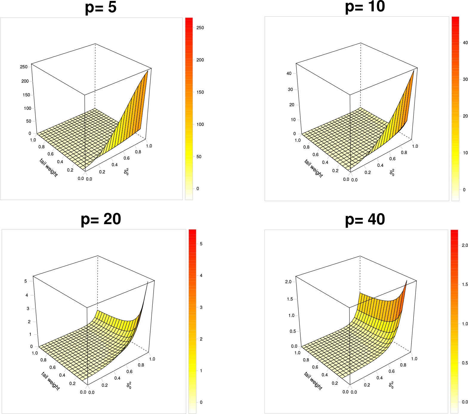
Figure 3 displays the heat color surfaces that depict the skewness measure γ1,pD as a function of the non-normality pair (β,δ*2) with 0 β ≤ 1 and δ*2=λ*21+λ*2 ranging in the interval [0,1). We can see that, due to the difficulties for computing large gamma functions in the expectations of the mixing variable, some blanks appear in the plots specially for the higher dimensions. Overall, it can be observed that the skewness decreases as the dimension increases. In addition, the curves on the skewness surface that trace the lines with equal tail weight show a dominance relation which means that, as the tail weight parameter β decreases, the corresponding skewness curve appear each one above the preceding one; this dominance relationship is illustrated by the plots displayed in Figure 4.

Figure 3.

Skewness surfaces with respect to the quantities δ*2=λ*21+λ*2 and the tail weight parameter β for dimensions p = 5 (top left), p = 10 (top right), p = 20 (bottom left) and p = 40 (bottom right).

Figure 4.

Skewness curves for the tail weight parameters: β = 3/4 (solid line), β = 1/2 (dashed line), β = 1/4 (dotted line) and dimensions p = 5 (top left), p = 10 (top right), p = 20 (bottom left) p = 40 (bottom right).

4. Concluding remarks

In this paper we have examined the multivariate skew exponential power distribution and have studied some of its theoretical properties in order to delve into the role played by the parameters of the model to handle the multivariate non-normality. It has been assumed that the tail weight parameter meets the condition 0 < β ≤ 1 so that the skew exponential power vector admits a SMSN stochastic representation. The SMSN formulation is useful to show that the tail weight parameter accounts for multivariate kurtosis regardless of the shape asymmetry vector, whereas the shape vector regulates the multivariate asymmetry in a directional fashion; specifically, it is shown that such a shape vector lies on the direction yielding the maximal skewness projection regardless of the value of the tail weight parameter. When the tail weight equals to β = 1, the underlying model reduces to the SN distribution and our result on directional skewness agrees with previous work for SN vectors [33]. Summing up, we advocate the unique and singular role of the tail weight and the shape vector of multivariate skew exponential power model to account independently for different facets of the non-normality.

The theoretical results from Theorems 3.1 and 3.2 have implications for research in the statistical practice including but not limited to: skewness-based projection pursuit, the modeling of non-normal asset returns, model-based clustering and the role played by the SEP parameters as well as the sensitivity of gaussian bayesian networks to deviations from normality along the lines of previous work [35]. Moreover, an explicit expression of the pdf of the SEP model would enable inferential work; research in this direction may benefit from the approach followed in Section 4.1 of [10].

Our findings also highlight some other problems for future research: A major advantage of the exponential power distribution is that it can model both light and heavy tails; as the Kotz-type distribution has the same characteristic and additionally it can also model holes [29], we wonder whether the properties studied for SEP distributions would also be valid for skewed generalizations of Kotz-type distributions. Moreover, the consideration of other SEP formulations, like those ones introduced in [2,12], may deserve further investigation on kurtosis assessment and directional skewness for the case β > 1. On the other hand, the skew-normal Cauchy model can be represented as a shape-scale mixture of SN distributions whose properties, including third moments and cumulants, have been investigated by [26] and are closely related to those ones of the SEP model; the study of directional asymmetry under shape-scale mixtures of SN vectors is also an open problem. Another issue is concerned with the consideration of other measures of multivariate skewness that depend on third moments [34].

As an afterthought, the results derived in this work also point out further research regarding the stochastic comparison of SMSN vectors: the SMSN representation of the multivariate skew exponential power model suggests looking into the role played by the non-normality parameters of the SMSN class by means of an ad hoc convex transform stochastic ordering; research effort along this line would complement previous related work on the issue [3, 5, 44].

(Communicated by Gejza Wimmer)

Appendix

proofs of auxiliary lemmas

Proof of Lemma 2.1.

The proof relies on a property about quadratic forms of SN vectors. Taking into account [11: Corollary 5.1] or the property appearing in expression (5.7) of [11: Section 5.7], we can assert that the quadratic form Q = (X – ξ)^┬Ω⁻¹(X – ξ) = S²Y^┬Ω⁻¹Y − with Y a vector such that Y ~ SN_p(0_p, Ω, α) – has the same distribution as S2Y0┬Ω−1Y0 with Y₀ a normal vector such that Y₀ ~ N_p(0_p, Ω). Hence, Q=dS2Y0┬Ω−1Y0=dS2G2, where G² is a scalar variable, independent of the mixing variable S, following a χp2 distribution. On the other hand, we also know that the quadratic form Q has the same distribution as the squared of the modular variable R associated to the p-dimensional elliptically contoured vector with distribution EP_p(ξ, Ω, β) [22]. The density function of R has been derived by [21]; it is given by

hR(r)=pΓ(1+p2β)2p2βrp−1exp{ −12r2β }I(o,∞)(r).

Since the scalar variables R² and Q have the same distribution, we can put:

E(Rk)=E(Sk)E(Gk).

from which we get

E(Sk)=E(Rk)E((G2)k/2).

The expectations appearing in E(S^k) can be calculated in an easy way due to the tractability of the density functions of R and G²; simple integral calculus gives

E(Rk)=2k/2βΓ(p+k2β)Γ(p2β)andE(Gk)=E((G2)k/2)=2k/2Γ(p+k2)Γ(p2)

which in turn leads to the expression of the statement. □

Proof of Lemma 3.1.

The result follows from the next property: if f and g are two increasing functions, then it holds that Cov(f(X), g(X)) ≥ 0 provided that the second order moments and cross moments of f(X) and g(X) exist. Since S is a non negative random variable the statement of the lemma will follow putting f(S) = S² and g(S) = S. □

Proof of Lemma 3.2.

Using the general expression from Lemma 2.1, we get

4.1 4πE(S)E(S3)−E(S2)2=22/βΓ2(p2)22Γ2(p2β)[ 4πΓ(p+12β)Γ(p+32β)Γ(p+12)Γ(p+32)−Γ2(p+22β)Γ2(p+22) ]=22/βp2Γ2(p+22β)Γ2(p2β)[ 4π2p+1Γ2(p+22)Γ2(p+12)Γ(p+12β)Γ(p+32β)Γ2(p+22β)−1 ].

We now define the function: g0(x)=g(x+ω2)−g(x) with g(x) = xψ(x), x ≥ 1, ω ≥ 1 and ψ the digamma function. This instrumental function will also be used in the proofs of Lemmas 3.2 and 3.3.

From the series expansion of the digamma function given by

ψ(z)=−γ−1z+∑n=1∞(1n−1n+z),

where γ is the Euler-Mascheroni constant, we obtain

g″(x)=2ψ′(x)+xψ″(x)=2∑n=1∞n(n+x)3.

Hence, g is a convex function which implies that g′(x) and g₀(x) are non decreasing functions, with the latter one being non decreasing because g0'(x)=g′(x+ω/2)−g′(x). Therefore,

g0(p2ω+ω)−g0(p2ω+ω2)=ω[ p+12ψ(p+12ω)−(p+2)ψ(p+22ω)+p+32ψ(p+32ω) ]=ω(log f(ω))′>0,

with f the function defined by f(ω)=Γ(p+12ω)Γ(p+32ω)Γ2(p+22ω), ω≥1, ω ≥ 1 and (log f(ω))′ its first log derivative.

The previous expression shows that f is non decreasing; so putting ω=1β, we get

f(1β)=Γ(p+12β)Γ(p+32β)Γ2(p+22β)≥f(1)=Γ(p+12)Γ(p+32)Γ2(p+22)=p+12Γ2(p+12)Γ2(p+22),

which implies that the quantity (4.1) is non negative, as we aimed to prove. □

Proof of Lemma 3.3.

From the general expression of the moments of the mixing variable in Lemma 2.1, we obtain after simple calculations

E(S3)+4πE(S)3−2E(S)E(S2)=2E(S)3[ 2π+f(ω) ],

where ω=1β and f is a function defined as follows:

f(ω)=Γ2(p+12)Γ2(p2)f1(ω)[f2(ω)−1],ω≥1

with f₁ and f₂ functions given by

f1(ω)=2Γ(p+22ω)Γ(p2ω)pΓ2(p+12ω)andf2(ω)=pΓ(p+32ω)Γ(p2ω)2(p+1)Γ(p+12ω)Γ(p+22ω).

Their first derivatives are

f1'(ω)=f1(ω)[ g0(p+12ω)−g0(p2ω) ]ωandf2'(ω)=f2(ω)[ g0(p+22ω)−g0(p2ω) ]ω.

with g₀ the same function as the one defined in the proof of the previous lemma. Using analogous arguments as before, we can conclude that f₁ and f₂ are non decreasing which implies

f1(ω)≥Γ2(p2)Γ2(p+12)andf2(ω)≥1/2.

We now calculate the first derivative of f:

f'(ω)=Γ2(p+12)Γ2(p2)f1(ω)×{ [ p+22ψ(p+22ω)+p2ψ(p2ω)−(p+1)ψ(p+12ω) ] [ f2(ω)−1 ]+f2(ω)[ p+32ψ(p+32ω)+p2ψ(p2ω)−p+12ψ(p+12ω)−p+22ψ(p+21ω) ] }.

Taking into account the lower bound for f₂, we get

Γ2(p2)Γ2(p+12)f′(ω)f1(ω)≥−12[p+22ψ(p+22ω)+p2ψ(p2ω)−(p+1)ψ(p+12ω)] +12[p+32ψ(p+32ω)+p2ψ(p2ω)−p+12ψ(p+12ω)−p+22ψ(p+22ω)]=12{p+32ψ(p+32ω)−(p+2)ψ(p+22ω)+p+12ψ(p+12ω)}=12ω{g0(p+22ω)−g0(p+12ω)}≥0.

Therefore, we can assert that f is also a non decreasing function for ω ≥ 1; consequently f(ω) ≥ f(1) = −1/2 which implies that

E(S3)+4πE(S)3−2E(S)E(S2)=2E(S)3[ 2π+f(ω) ]≥2E(S)3[ 2π−12 ]≥0

as we aimed to prove. □

Acknowledgement

The authors are grateful to the reviewers for their useful recommendations that contributed to improve the draft version of this paper. JMA also acknowledges the support received by NextGenerationEU.

References

[1] Agrò, G.: Maximum likelihood estimation for the exponential power function parameters, Comm. Statist. Simulation Comput. 24(2) 1995, 523–536.10.1080/03610919508813255Search in Google Scholar

[2] Arellano-Valle, R.—Richter, W.-D.: On skewed continuous l_n,p-symmetric distributions, Chil. J. Stat. 3 (2012), 193–212.Search in Google Scholar

[3] Arevalillo, J. M.—Navarro, H.: A study of the effect of kurtosis on discriminant analysis under elliptical populations, Multivariate Anal. 107 (2012), 53–63.10.1016/j.jmva.2012.01.011Search in Google Scholar

[4] Arevalillo, J. M.—Navarro, H.: A note on the direction maximizing skewness in multivariate skew-t vectors, Statist. Probab. Lett. 96 (2015), 328–332.10.1016/j.spl.2014.10.014Search in Google Scholar

[5] Arevalillo, J. M.—Navarro, H.: A stochastic ordering based on the canonical transformation of skew-normal vectors, TEST 28(2) (2019), 475–498.10.1007/s11749-018-0583-5Search in Google Scholar

[6] Azzalini, A.: Further results on a class of distributions which includes the normal ones, Statistica 46 199-208, 1986; Reprinted with annotations and corrigenda 80 (2020), 161–175.Search in Google Scholar

[7] Azzalini, A.: The R package sn: The Skew-Normal and Related Distributions such as the Skew-t and the SUN (version 2.0.0), Università di Padova, Italia, 2021.Search in Google Scholar

[8] Azzalini, A.—Capitanio, A.: Statistical applications of the multivariate skew normal distribution, J. R. Stat. Soc. Ser. B. Stat. Methodol. 61(3) (1999), 579–602.10.1111/1467-9868.00194Search in Google Scholar

[9] Azzalini, A.—Dalla Valle, A.: The multivariate skew-normal distribution, Biometrika 83(4) (1996), 715–726.10.1093/biomet/83.4.715Search in Google Scholar

[10] Azzalini, A.—Capitanio, A.: Distributions generated by perturbation of symmetry with emphasis on a multivariate skew t-distribution, J. R. Stat. Soc. Ser. B. Stat. Methodol. 65(2) (2003), 367–389.10.1111/1467-9868.00391Search in Google Scholar

[11] Azzalini, A.—Capitanio, A.: The Skew-Normal and Related Families. IMS Monographs, Cambridge University Press, 2014.10.1017/CBO9781139248891Search in Google Scholar

[12] Azzalini, A.—Regoli, G: Some properties of skew-symmetric distributions, Ann. Inst. Statist. Math. 64(4) (2012), 857–879.10.1007/s10463-011-0338-5Search in Google Scholar

[13] Box, G. E. P.: A note on regions for tests of kurtosis, Biometrika 40(3–4) (1953), 465–468.10.1093/biomet/40.3-4.465Search in Google Scholar

[14] Box, G. E. P.—Tiao, G. C.: Bayesian Inference in Statistical Analysis, Addison-Wesley Publishing Company, 1973.Search in Google Scholar

[15] Branco, M. D.—Dey, D. K.: A general class of multivariate skew-elliptical distributions, J. Multivariate Anal. 79(1) (2001), 99–113.10.1006/jmva.2000.1960Search in Google Scholar

[16] Capitanio, A: On the canonical form of scale mixtures of skew-normal distributions, https://arxiv.org/abs/1207.0797.Search in Google Scholar

[17] Capitanio, A: On the canonical form of scale mixtures of skew-normal distributions, Statistica 80(2) (2020), 145–160.Search in Google Scholar

[18] Choy, S. T. B.—Smith, A. F. M.: Hierarchical models with scale mixtures of normal distributions, TEST 6(1) (1997), 205–221.10.1007/BF02564434Search in Google Scholar

[19] Fang, K. T.—Kotz, S.—NG, K.-W.: Symmetric Multivariate and Related Distributions. Monographs on Satistics and Applied Probability, Chapman & Hall, 1990.10.1007/978-1-4899-2937-2Search in Google Scholar

[20] Gómez-Villegas, M. A.—Main, P.—Navarro, H.—Susi, R.: Assessing the effect of kurtosis deviations from gaussianity on conditional distributions, Appl. Math. Comput. 219(21) (2013), 10499–10505.10.1016/j.amc.2013.04.031Search in Google Scholar

[21] Gómez, E.—Gómez-Villegas, M. A.—Marín, J. M.: A multivariate generalization of the power exponential family of distributions, Comm. Statist. Theory Methods 27(3) (1998), 589–600.10.1080/03610929808832115Search in Google Scholar

[22] Gómez-Sánchez-Manzano, E.—Gómez-Villegas, M. A.—Marín, J. M.: Sequences of elliptical distributions and mixtures of normal distributions, J. Multivariate Anal. 97(2) (2006), 295–310.10.1016/j.jmva.2005.03.008Search in Google Scholar

[23] Gómez-Sánchez-Manzano, E.—Gómez-Villegas, M. A.—Marín, J. M.: Multivariate exponential power distributions as mixtures of normal distributions with bayesian applications, Comm. Statist. Theory Methods 37(6) (2008), 972–985.10.1080/03610920701762754Search in Google Scholar

[24] Goodman, I. R.—Kotz, S.: Multivariate θ-generalized normal distributions, J. Multivariate Anal. 3(2) (1973), 204–219.10.1016/0047-259X(73)90023-7Search in Google Scholar

[25] Hazan, A.—Landsman, Z.—Makov, U. E.: Robustness via a mixture of exponential power distributions, Comput. Statist. Data Anal. 42(1) (2003), 111–121.10.1016/S0167-9473(02)00153-6Search in Google Scholar

[26] Kahrari, F.—Rezaei, M.—Yousefzadeh, F.—Arellano-Valle, R. B.: On the multivariate skew-normal-cauchy distribution, Statist. Probab. Lett. 117 (2016), 80–88.10.1016/j.spl.2016.05.005Search in Google Scholar

[27] Kano, Y.: Consistency property of elliptic probability density functions, J. Multivariate Anal. 51(1) (1994), 139–147.10.1006/jmva.1994.1054Search in Google Scholar

[28] Kim, H.-M.—Kim, C.: Moments of scale mixtures of skew-normal distributions and their quadratic forms, Comm. Statist. Theory Methods 46(3) (2017), 1117–1126.10.1080/03610926.2015.1011339Search in Google Scholar

[29] Kollo, T.—Roos, A.: On Kotz-type elliptical distributions, In: Contemporary Multivariate Analysis and Design of Experiments, World Scientific, 2005, pp. 159–170.10.1142/9789812567765_0010Search in Google Scholar

[30] Korolev, V.: Some properties of univariate and multivariate exponential power distributions and related topics, Mathematics 8(11) (2020), Art. No. 1918.10.3390/math8111918Search in Google Scholar

[31] Kotz, S.: Multivariate distributions at a cross road. In: A Modern Course on Statistical Distributions in Scientific Work (G. P. Patil, S. Kotz, and J. K. Ord, eds.), Springer Netherlands, Dordrecht, 1975, pp. 247–270.10.1007/978-94-010-1842-5_20Search in Google Scholar

[32] Kuwana, Y.—Kariya, T.: Lbi tests for multivariate normality in exponential power distributions, J. Multivariate Anal. 39(1) (1991), 117–134.10.1016/0047-259X(91)90009-QSearch in Google Scholar

[33] Loperfido, N.: Canonical transformations of skew-normal variates, TEST 19(1) (2010), 146–165.10.1007/s11749-009-0146-xSearch in Google Scholar

[34] Loperfido, N.: Singular value decomposition of the third multivariate moment, Linear Algebra Appl. 473(2015), 202–216.10.1016/j.laa.2014.05.043Search in Google Scholar

[35] Main, P.—Navarro, H.: Analyzing the effect of introducing a kurtosis parameter in gaussian bayesian networks, Reliab. Eng. Syst. Safety 94(5) (2009), 922–926.10.1016/j.ress.2008.10.004Search in Google Scholar

[36] Malkovich, J. F.— Afifi, A. A.: On tests for multivariate normality, J. American Statist. Assoc. 68(341) (1973), 176–179.10.1080/01621459.1973.10481358Search in Google Scholar

[37] Morán-Vásquez, R. A.—Ferrari, S. L. P.: Box–cox elliptical distributions with application, Metrika 82(5) (2019), 547–571.10.1007/s00184-018-0682-zSearch in Google Scholar

[38] Morán-Vásquez, R. A.—Ferrari, S. L. P.: New results on truncated elliptical distributions, Commun. Math. Stat. 9(3) (2021), 299–313.10.1007/s40304-019-00194-3Search in Google Scholar

[39] NADARAJAH, S.: A generalized normal distribution, J. Appl. Stat. 32(7) (2005), 685-694.10.1080/02664760500079464Search in Google Scholar

[40] Sánchez-Manzano, E. G.—Gómez-Villegas, M. A.—Marín-Diazaraque, J.-M.: A matrix variate generalization of the power exponential family of distributions, Comm. Statist. Theory Methods 31(12) (2002), 2167-2182.10.1081/STA-120017219Search in Google Scholar

[41] Simoni, S.: Su una estensione dello schema delle curve normali di ordina r alle variabili doppie, Statistica 28 (1968), 151–170.Search in Google Scholar

[42] Subbotin, M. T.: On the law of frequency of error, Mat. Sbornik 31(2) (1923), 296–301.Search in Google Scholar

[43] Van Zwet, W. R.: Convex Transformations of Random Variables, Mathematish Centrum, Amsterdam, 1964.Search in Google Scholar

[44] Wang, J: A family of kurtosis orderings for multivariate distributions, J. Multivariate Anal. 100(3) (2009), 509–517.10.1016/j.jmva.2008.06.001Search in Google Scholar

[45] Wang, M.—Lu, T.: A matching prior for the shape parameter of the exponential power distribution, Statist. Probab. Lett. 97 (2015), 150–154.10.1016/j.spl.2014.11.016Search in Google Scholar

[46] West, M.: On scale mixtures of normal distributions, Biometrika 74(3) (1987), 646–648.10.1093/biomet/74.3.646Search in Google Scholar

Received: 2022-01-11

Accepted: 2022-06-02

Published Online: 2023-03-31

Published in Print: 2023-04-01

This work is licensed under the Creative Commons Attribution 4.0 International License.

Articles in the same Issue

https://doi.org/10.1515/ms-2023-0039

Keywords for this article

Skew exponential power; asymmetry; skewness; tail weight; kurtosis

Creative Commons

BY 4.0