Deep learning-based image super resolution methods in microscopy – a review
-
Andreas Jansche

 ,
Patrick Krawczyk
,
Miguelangel Balaguera
,
Anoop Kini
,
Timo Bernthaler
und
Gerhard Schneider
,
Patrick Krawczyk
,
Miguelangel Balaguera
,
Anoop Kini
,
Timo Bernthaler
und
Gerhard Schneider

Abstract
Deep learning-based image super resolution (SR) is an image processing technique designed to enhance the resolution of digital images. With the continuous improvement of methods and the growing availability of large real-world datasets, this technology has gained significant importance in a wide variety of research fields in recent years. In this paper, we present a comprehensive review of promising developments in deep learning-based image super resolution. First, we give an overview of contributions outside the field of microscopy before focusing on the specific application areas of light optical microscopy, fluorescence microscopy and scanning electron microscopy. Using selected examples, we demonstrate how the application of deep learning-based image super resolution techniques has resulted in substantial improvements to specific use cases. Additionally, we provide a structured analysis of the architectures used, evaluation metrics, error functions, and more. Finally, we discuss current trends, existing challenges, and offer guidance for selecting suitable methods.
1 Introduction
From a conventional perspective, super resolution in microscopy refers to an imaging technique that achieves a higher resolution than traditional light optical microscopy. In particular, approaches such as stimulated emission depletion (STED) microscopy [1], structured illumination microscopy (SIM) [2] and stochastic optical reconstruction microscopy (STORM) [3] are well known. However, this review paper is dedicated to an alternative method for generating high-resolution images: deep learning-based image super resolution (SR). This method is independent of the acquisition technique and is therefore used in light optical microscopy [4], [5], [6], [7], [8] including fluorescence microscopy [9], [10], [11], [12], [13], [14] and other imaging techniques such as scanning electron microscopy [8], [15], [16], [17], [18], [19], [20] and ultrasound localization microscopy [21]. It is even possible to combine conventional imaging techniques for super resolution (like STED, SIM, STORM) with the deep learning-based image super resolution presented in this work [5], [6]. The approach is based on the digital upscaling of images by a trained deep learning model, which can be done either in situ during the acquisition or for already acquired images in a post-processing step. This makes image SR using deep learning an extremely flexible and versatile method for image quality enhancement in spatial resolutions (minimal separation distance between two objects with high contrast points), temporal resolutions (frequency at which images can be retrieved) and even for noise reduction [22].
Our focus in this review paper is on the application of deep learning-based image super resolution specifically in the field of microscopy. The aim is to provide a comprehensive overview of the scenarios in which this technology is used and the added value its application offers. Compared to other super resolution review publications, which mainly focus on technical aspects, improvement of conventional SR methods or other domains [23], [24], [25], [26], [27], [28], [29], [30] this review aims towards the detailed consideration of microscopy-specific applications.
The main contribution of this work is as follows:
We provide a comprehensive survey of image super resolution methods as well as their applications. We describe and show how super resolution has enabled significant improvements.
We provide a systematic overview of the available methods, their areas of application, as well as the datasets and metrics used.
Finally, we discuss current trends, existing challenges, and provide guidance for the selection of suitable methods.
Furthermore, the review is structured as follows to provide a comprehensive understanding of both the basic methods and their specific applications.
Fundamentals: Provides an explanation of the most important terms and concepts. It provides a general overview of different architectural designs for deep learning-based image super resolution and illustrates their successful application outside of microscopy.
Deep learning-based image super resolution in microscopy: The emphasis in this section is on the application of super resolution methods in microscopy, with a particular focus on light optical microscopy and scanning electron microscopy.
Summary: In this section we provide the special characteristics of the deep learning-based image super resolution methods derived from this literature review.
Challenges and Opportunities: This section provides final thoughts on the challenges and opportunities of image super resolution using deep learning methods, focusing on real-world data, evaluation metrics, loss functions and architectures.
2 Fundamentals
2.1 Problem definition
The aim of deep learning-based image super resolution is to reconstruct a high-resolution image from a low-resolution image, which can be described by the formula in Equation (1).
Problem definition of image super resolution.
where IHR represents the high-resolution image, ILR the low-resolution image, N the noise factor based on the acquisition system and ↑(*) the upsampling method, which is the focus of this literature survey. The upsampling of images is an ill-posed problem, as there are theoretically an infinite number of possible results for the interpolation and reconstruction of individual pixel values. In other words, image super resolution is based on an estimate of what the original, low-resolution image might look like in an enlarged version. Therefore, the reconstruction result should be interpreted with caution. It is essential to carefully validate the trained deep learning models with respect to their specific use case.
2.2 Terminology and concepts
This chapter is intended to help introduce the topic of image super resolution by providing a brief summary of important keywords and their descriptions.
2.2.1 Convolutional Neural Networks (CNN)
A Convolutional Neural Network (CNN) uses filters to extract local features such as edges and textures from an image with a sliding window (Figure 1). During training, the filters are dynamically adjusted so that the network learns to recognize relevant features for a specific task. A typical CNN consists of a convolutional layer, an activation function and an up- or downsampling layer. This modular structure makes it possible to implement a wide variety of architectures that can be adapted to specific requirements. A very common CNN architecture are encoder-decoder networks like U-Net, that consist of an encoder network to extract and condense relevant image features into a so-called latent space representation and a decoder network (similar to the one shown in Figure 1, often a symmetrical inverse of the encoder) that reconstructs an image from a latent space representation.

Schematic illustration of a CNN architecture using the example of a decoder that generates a higher resolution from a lower resolution. In the figure, the size of the feature maps (colored) increases as the layers progress, while the number of feature maps decreases. The white square within the feature maps is the learned filter, with each feature map having its own filter.
In the field of image super resolution, Dong et al. [31] presented one of the first CNN models called SRCNN, whose convolutional filters have learned a function to map an LR image to an HR image. The fact that an HR output is directly generated from an LR input makes the model one of the first end-to-end models. To ensure that their model can also be used for real-time requirements, the authors optimized their first model SRCNN for speed and named it Fast Super-Resolution Convolutional Neural Network (FSRCNN) [32]. They achieved a speed improvement of roughly 40× without sacrificing quality and were able to upscale videos to 720p with 24 fps by directly using the LR as input and reducing the filter sizes to 3×3. A further advance was achieved by the authors Berger et al. [33] with QuickSRNet which extracts architecture features from a VGG-like structure, without input-to-output residual connections. The authors claimed that their architecture produces 1080p outputs via 2× upscaling in only 2.2 ms for a single frame on a modern smartphone, which makes it ideal for high-fps real-time applications.
2.2.2 Generative Adversarial Networks (GAN)
A Generative Adversarial Network (GAN) consists of two networks: a generator and a discriminator (Figure 2). These are involved in an adversarial learning process in which the generator attempts to deceive the discriminator, while the discriminator becomes continuously better at recognizing generated data. During training, the generator improves and produces more realistic images over time. During inference, the discriminator is no longer needed and only the generator is used. In image super resolution, the generator produces a HR image from a LR image.

Schematic illustration of a training processes of a GAN architecture. The generator generates a new HR image from an LR image. The discriminator tries to distinguish between real and fake images. Eventually the generator learns to generate realistic images.
One of the first GAN architectures for image super resolution was the Super-Resolution GAN (SRGAN) proposed by Ledig et al. [34]. SRGAN comprises a generator based on residual networks and incorporates perceptual loss for texture recovery in the generated HR images. SRGAN effectively upscales images by a factor of 4× while maintaining perceptual quality. The authors emphasized the focus of this work for perceptual quality rather than computational efficiency. Using the performance metric mean opinion score (MOS), SRGAN outperformed its predecessors, as shown on datasets like Set5 [35], Set14 [36], and BSD 100 [37]. Wang et al. [38] proposed ESRGAN, an architecture based on SRGAN, with a residual-in-residual dense block (RRDB) architecture not using batch normalization. It allowed for better feature extraction and improved visual quality in the generated images. It also utilizes a perceptual loss function that focuses on high-level features extracted from pre-trained networks, as a final remark ESRGAN has been also used in other works such as [8], [39]. CycleGAN [40] proposed by Zhu et al. is another example, although primarily known for style transfer, can also be adapted for super resolution tasks by learning to map low-resolution images to high-resolution counterparts even without requiring paired training data. In the landscape of GAN models, Conditional GAN (CGAN) [41] is another variant that incorporates additional information (like class labels) into the GAN framework. This can be beneficial for certain super resolution tasks where conditional information is also available.
2.2.3 Transformer
Transformer models have overtaken CNNs and GANs and are now considered state-of-the-art in many areas of image processing. Their success is primarily based on self-attention layers and good scalability. In contrast to CNNs, which can only capture local dependencies through their filters, self-attention enables the capture of global dependencies. This means that information from different image areas can be processed together. Figure 3 shows a self-attention layer. The input is first transformed into query, key and value. The similarity between query and key is then calculated. Finally, the values are summed up in a weighted manner to generate a new representation of the input. An extended concept is multi-head attention, in which several self-attention modules are stacked. Each head can focus on different features, allowing the model to perform a more comprehensive analysis of the input information.
![Figure 3:
Schematic illustration of a self-attention module, as is commonly used in a Transformer model. Key, query and value are labeled K, Q and V respectively, and []T indicates a transposed matrix.](/document/doi/10.1515/mim-2024-0032/asset/graphic/j_mim-2024-0032_fig_003.jpg)
Schematic illustration of a self-attention module, as is commonly used in a Transformer model. Key, query and value are labeled K, Q and V respectively, and []T indicates a transposed matrix.
One of the first transformer models for image super resolution was introduced by Yang et al. with TTSR [42]. This model belongs to the field of reference-based super-resolution. During training, an HR image is used in addition to the LR image to transfer features. Even after training, the model requires an HR image that is similar to the input image in terms of colors and textures. The Swin Transformer, developed by Liu et al. [43], achieves state-of-the-art results without requiring an HR image as additional input. By applying local self-attention mechanisms in a hierarchical structure, the model reduces the computational complexity compared to vision transformer approaches. The linear computational complexity in relation to the image size makes the Swin Transformer very efficient. Forigua et al. [44] have adapted the Swin Transformer for 3D data and developed the SuperFormer model. This model was specifically designed for volumetric medical imaging, for example for MRI scans. SuperFormer integrates local self-attention mechanisms and 3D-relative position coding to enable high-resolution 3D reconstructions with fine details. In addition, the Efficient Super-Resolution Transformer (ESRT) by Lu et al. [45] combines a Lightweight Transformer Backbone (LTB) with a Lightweight CNN Backbone (LCB). As a result, long-range dependencies are captured while the computational effort remains low. The unique selling point of this work lies in lower memory requirements. Compared with the original Transformer [46] which occupies 16 GB GPU memory, ESRT needed 4 GB of GPU memory during training with a patch size of 48×48 and a batch size of 16. The Multi-Attention Fusion Transformer (MAFT) proposed by Li et al. [47] integrates multiple attention mechanisms for improved reconstruction of super-resolved images. By attempting to balance the dependency between short-term and long-term spatial information, shifted windows are introduced, leading to better image quality. Compared to state-of-the-art methods, the proposed MAFT achieved 0.09 dB gains on the Urban100 [48] dataset for 4× SR task while containing merely 32.55 % fewer parameters and 38.01 % lower floating-point operations (FLOPs), respectively. Most recently Bommanapally et al. [8] used popular state of the art transformer-based super resolution techniques SwinIR [49] and HAT [50], to evaluate their performance in different deep learning approaches, using supervised, contrastive and noncontrastive self-supervised learning. They found that when using SR images, the supervised and self-supervised approach outperforms by 2–6 % those architectures that do not use SR images. This demonstrates the versatility of implementation that transformers architectures might have in super-resolution related tasks.
2.2.4 Diffusion models
A diffusion model is a generative model that is divided into two phases. In the first phase, noise is gradually added to the LR image until no original image information is apparent. In the second phase, the first process is reversed. Deep learning models are used which gradually reduce the noise in order to produce an HR image. However, the calculation is very time-consuming as it consists of many individual steps. More recent models therefore use an encoder to transfer the input image into the latent space, which makes the process more efficient. The entire process is illustrated in Figure 4.
![Figure 4:
Schematic illustration of a diffusion model operating in latent space. Z represents a feature map in the latent space, T represents the number of steps in the diffusion process. The DL model (deep learning model, often a U-Net) gradually reduces the noise. The schematic is a simplified representation of the architecture from [51].](/document/doi/10.1515/mim-2024-0032/asset/graphic/j_mim-2024-0032_fig_004.jpg)
Schematic illustration of a diffusion model operating in latent space. Z represents a feature map in the latent space, T represents the number of steps in the diffusion process. The DL model (deep learning model, often a U-Net) gradually reduces the noise. The schematic is a simplified representation of the architecture from [51].
The first diffusion models for image super resolution include SR3 [52], IDM [53] and ResShift [54]. SR3 proposed by Saharia et al. was developed specifically for general data and focuses particularly on the super resolution of faces and nature images. It uses a U-Net model for noise reduction and can upsample images from 64×64 to 256×256 and from 256×256 to 1024×1024. In a survey with participants, the generated images achieved a fool rate of 50 %. IDM proposed by Gao et al. was tested on the same datasets as SR3 and showed improved performance. Unlike SR3, IDM uses only the encoder of the U-Net for noise reduction, while the decoder was replaced by a special architecture for an implicit neural representation. In addition, a coordinate-based multi-layer perceptron (MLP) is used to encode images as features in continuous space, enabling highly detailed reconstructions. Another advantage of IDM is its flexible scaling: while conventional methods often only support scaling factors of exponents of 2, for instance of 4× or 16×, IDM also enables any intermediate levels such as a 10× magnification. ResShift proposed by Yue et al. takes a different approach by reducing the number of diffusion steps to make the super resolution process more efficient. It does this by using a Markov chain that shifts the residual between HR and LR images to improve transition efficiency. In addition, ResShift has a flexible noise scheduler that adjusts the shifting speed and noise strength during the diffusion process to achieve a better balance between image quality and computational effort. Recently, Cheng et al. [55] proposed DiT-SR, an diffusion transformer that adopts a U-shaped architecture for multi-scale hierarchical feature extraction. It uses a uniform isotropic design for transformer blocks across different stages. A frequency-adaptive time-step conditioning module also gets incorporated for improved processing of distinct frequency information during the diffusion process.
2.2.5 Up- and downsampling
In the field of image super resolution, which aims to increase the resolution of an image, upsampling methods play a central role. These can be divided into two categories: Fixed methods and learnable methods. Fixed methods upsample an image or a feature map based on predefined calculation parameters. Well-known algorithms are bilinear and bicubic interpolation, resize convolution, unpooling (max unpooling, average unpooling), nearest-neighbor and sub-pixel convolution [56]. Compared to fixed methods, learnable methods such as deconvolution and Meta-Upscale Module [57] adapt dynamically during training. The downsampling of images and feature maps can also be divided into fixed methods such as pooling layers (max pooling, average pooling), wavelet transformations and anti-aliasing filters, as well as methods that can be learned such as strided convolutions.
Finally, a detailed analysis of the advantages and disadvantages of the algorithms is presented in the summary of this paper.
2.2.6 Loss functions
The loss function is one of the most important hyperparameters when training a model. It plays a central role in evaluating the deviation between the output generated by the model and the actual training labels. A high deviation is penalized by the loss function more than a low one, forcing the model to update its parameters to minimize errors and improve accuracy. There are two main categories of loss functions: pixel-based and perceptual-based loss functions.
Pixel-based loss functions calculate the direct deviation between the pixel values of the model prediction and those of the label. They are widely used and are almost always applied. Well-known pixel-based error functions include the mean absolute error (MAE, L1), the mean squared error (MSE, L2), root mean squared error (RMSE), binary cross entropy loss (BCE) and dice coefficient. In addition to these common loss functions, there are also specialized variants such as the Carbonnier Loss, the Barlow Twins Loss and the Cosine Similarity, which can be preferred depending on the use case.
However, pixel-based loss functions do not capture human perception very well, which is why perception-based loss functions are being developed specifically for this purpose. These compare extracted features of the model prediction with those of the training label. As with pixel-based error functions, larger deviations are penalized more heavily. One of the most well-known perceptual loss functions is based on the VGG network and was developed by K. Simonyan and A. Zisserman of the Visual Geometry Group (VGG) at Oxford University – hence the name VGG [58]. Originally designed as a convolutional network for object recognition, it has been widely used due to its high performance and free availability. The architecture of the VGG network enables the extraction of deep features, making it particularly well suited for perceptual error features.
The training of a model can be significantly improved by selecting the right loss function or rather combination of loss functions, since it has a direct influence on the adaptation of the model parameters and thus on the model performance.
2.2.7 Performance metrics
Metrics are used to evaluate the performance of a trained model. The literature offers a variety of such metrics for different application areas. These can be roughly divided into two categories: Reference-based and non-reference-based metrics. The difference is that reference-based metrics require a reference to evaluate a comparison or performance. In contrast, non-reference-based metrics do not require a reference; these metrics can be applied directly to the model output. The most well-known non-reference-based metrics include Perception-Based Image Quality Evaluator (PIQE) [59], Natural Image Quality Evaluator (NIQE) [60] and Blind/Referenceless Image Spatial Quality Evaluator (BRISQUE) [61].
Similar to the loss functions, reference-based metrics can be divided into two categories: Distortion-based and perceptual-based metrics. It is noteworthy that loss functions described above are also listed as reference-based metrics. In principle, metrics can be used as loss functions and vice versa - however, the model training could become unstable. Distortion-based metrics are often based on pixel or frequency-based methods. Well-known representatives are Peak Signal-to-Noise Ratio (PSNR), MAE, MSE, RMSE, Structural Similarity Index Measure (SSIM) and Multi-Scale Structural Similarity Index Measure (MS-SSIM). The perceptual-based metrics, which also include feature-based metrics, include Learned Perceptual Image Patch Similarity (LPIPS) [62], PieAPP [63], SAMScore [64], Inception Score (IS) and Fréchet Inception Distance (FID) [65].
A detailed description of the advantages and disadvantages of these metrics can be found in the Summary and in the Challenges and Opportunities section at the end of this paper.
2.2.8 Geometric registration approach
Geometric registration is a very important topic for image super resolution. The aim is to ensure that the positions of the structures in the low-resolution image (LR) match the positions of the structures in the high-resolution image. The better the match, the more promising the model training. The simplest approach of geometric registration is with synthetic datasets. Here, the HR images are downsampled, which ensures that there is a match between LR and HR. A problem only arises with real datasets. Depending on the acquisition technique, a match between LR and HR can lead to extreme overhead. A one hundred percent match is often not feasible due to the tolerances of the acquisition system, which is why the training data already contains deviations. Fortunately, this does not mean that the model training is unsuccessful. However, the model performance decreases with increasing deviation in the dataset. In the summary section the subject of geometric registration is addressed again.
3 Deep learning-based image super resolution in microscopy
Besides the factors governing the performance of deep-learning-based super resolution methods, and its potential applications in microscopy such as optimization of imaging parameters, image denoising, acceleration of image speed and cross-modality super-resolution reconstruction [66], this section aims to show the different approaches that have been developed to implement deep learning-based image super resolution techniques for quality enhancement of microscopy images.
3.1 Light optical microscopy
In classical light optical microscopy, the optical resolution indicates the minimum distance at which two closely spaced points still appear as separate units in the image. As originally proposed, the resolution is limited by the Abbe diffraction limit, which is around 200 nm for visible light [67]. This limit is determined by the wavelength of the light used and the numerical aperture (NA) of the objective. Fluorescence microscopy, which is a variant of light optical microscopy, is one of the most popular techniques in the field of biology. This is given that this method possesses a high sensitivity, specificity (ability to specifically mark molecules and structures of interest), and simplicity, which makes it possible to be used on living cells and organisms [68]. This technique also has different modalities, such as widefield where the entire sample is exposed to the light source whenever there is a change of position in the axial direction [69], light-field which uses light field theory to scan volumetric images of the sample at high speed [70], bright-field which is considered one of the simplest techniques, where the sample is illuminated throughout and the visual contrast is facilitated when the light is absorbed in its denser areas [71], and finally, dark-field technique that enhances contrast in materials which are difficult to image under normal lighting conditions by using oblique illumination [72]. Even though the existing limitations of this techniques might undermine the generation of images with an appropriate contrasts and higher quality, modern deep learning-based image super resolution methods offer the possibility to help overcome both the Abbe’s diffraction limit and these limitations to significantly improve the image [73].
3.1.1 Convolutional neural networks
One case of a successful implementation is found in Nehme et al. [12] where they designed an approach that uses a deep convolutional neural network which is trained and evaluated with both simulated and experimental data of blinking emitters. To generate the simulated data they used the ThunderSTORM plugin [74] and ImageJ which is a popular digital image processing software [75], [76]. The experimental data was collected using SMLM (single-molecule localization microscopy) technique with an inverted fluorescence microscope. Furthermore, in order to achieve a variety of SNRs and emitter densities, images were taken with several levels of laser powers and combined in post processing. The architecture of this approach encodes the image into a dense, aggregated feature representation, through three 3×3 convolutional layers with increasing depth, interleaved with 2×2 max-pooling layers. Subsequently the output goes through the decoding stage, which has three successive deconvolution layers, each consisting of 2×2 up-sampling modules, interleaved with 3×3 convolutional layers with decreasing depth. Here the spatial dimensions are processed in order to have the same shape as the input image.
A representation of the model’s capabilities on image reconstruction can be seen in Figure 5(II). Results of this work report microtubule reconstructions obtained on a 12.5 nm pixel grid and QD reconstructions on a grid with a 13.75 nm pixel size. Furthermore, the authors reported an increment in the minimal resolvable distance between stripes behaving as a function of emitter density with values ranging from at least 19 nm for 1
![Figure 5:
The encoder-decoder CNN Deep-STORM. (I) Simple depiction of the Deep-STORM model for super resolution. (II) Examples of the diffraction limited input images (a) and a super-resolved result (b) [12].](/document/doi/10.1515/mim-2024-0032/asset/graphic/j_mim-2024-0032_fig_005.jpg)
The encoder-decoder CNN Deep-STORM. (I) Simple depiction of the Deep-STORM model for super resolution. (II) Examples of the diffraction limited input images (a) and a super-resolved result (b) [12].
Later in 2021, Vizcaíno et al. [78] presented a deep learning approach to reconstruct confocal microscopy 3D image stacks of mouse brain with the size of 1287×1287×64 voxels (112×112×57.6 µm3) from a single light field image of size 1287×1287 pixels. Their network called LFMNet has a first layer with a 4D convolutional layer, the image that is output by this is converted to a 2D image trough a mapping function, later a U-Net carries out convolutions as downscaling operators, completes the feature extractions and then the 3D reconstruction. In order to assess the performance of their method they compared two different variants of its network architecture a shallow U-Net composed by 2 down/up-sample operations with a receptive field of 19 pixels and a full U-Net composed by 4 down/up-sample operations with a receptive field of 104 pixels. Then they measured the PSNR and SSIM metrics to quantify the improvements and identify which had the best performance on reconstructing a HR version of the ground truth. For instance, their shallow model in the final design outperforms the remaining methods with a PSNR value of 34.45 and a SSIM index of 0.87 and a time for reconstructing a super-resolved image of 20 ms. Based on these results and their analysis they demonstrated that by using the appropriate deep learning model they can reduce considerably the image acquisition time, and improve the capability for imaging in highly dynamic and light-sensitive events, such as live cells and biology-related tasks in general.
Furthermore, transfer learning has taken participation in super resolution enhancement proceedings in microscopy. Christensen et al. [79] created a method called ML-SIM that aimed to work out the drawbacks of traditional SIM reconstruction process, these being time consuming and tendency to produce artefacts especially for images with low signal-to-noise ratios, which is a scenario where traditional methods would produce the wrong reconstructions by confusing noise as signal. The proposed methodology uses transfer learning, with a parameter-free model that aims to generalize further in the reconstruction process of data recorded by a determined imaging device as well as a specific sample type. They selected RCAN [80] as the baseline for their the ML-SIM architecture, which has around 100 convolutional layers and 10 residual groups with 3 residual blocks. The model was trained with the DIV2K image dataset which is a popular repository used by other authors in the field. Additionally, they generated synthetic data so they were able to use it as input as well for the supervised learning approach.
In the evaluation stage of their approach, they compared the wide-field image with the reconstructed version produced by their approach. They observed a noticeable resolution improvement, quantified by a PSNR increase of over 7 dB and a SSIM index that was 28.09 % higher. A visual representation of this improvements can be seen in Figure 6. These outcomes show that ML-SIM reconstructions contain less noise and a considerably reduced number of artefacts than the other methods, it also improves visual quality in terms of resolution which benefits the structured illumination microscopy image acquisition process and can potentially be used in biology and cellular studies that involve SIM.
![Figure 6:
ML-SIM results compared to OpenSIM, CC-SIM and FairSIM, with the original wide-field input image on the left. Fluorescent beads, as well as the endoplasmic reticulum and cell membrane [79]. (Image cropped from the original version).](/document/doi/10.1515/mim-2024-0032/asset/graphic/j_mim-2024-0032_fig_006.jpg)
ML-SIM results compared to OpenSIM, CC-SIM and FairSIM, with the original wide-field input image on the left. Fluorescent beads, as well as the endoplasmic reticulum and cell membrane [79]. (Image cropped from the original version).
Further work was developed by Shah et al. [6] proposing a residual convolutional neural network (RED-Net) designed to denoise and reconstruct data generated with SIM microscopy. In the first part of their work, they introduce an end-to-end architecture along with a baseline related to existing work combining SIM and deep learning. They proposed a network called super resolution residual encoder–decoder structured illumination microscopy (SR-REDSIM), which takes raw SIM images as input and generates a super-resolved image as output. In the second part, they presented Residual Encoder–Decoder FairSIM (REDfairSIM), which combines standard computational SIM reconstruction with a deep learning network. This method focuses on reconstructing images using typical frequency-domain algorithms while leveraging a deep convolutional neural network for artifact reduction and denoising. In addition to the aforementioned, they also provide a workflow called preRED-fairSIM, where deep learning is applied to the raw SIM images for denoising before SIM reconstruction. This approach aimed to evaluate the model’s generalization capabilities under four different noise levels: level 0 for the highest SNR at timestamp 0, level 1 for timestamps 25–40 level 2 for timestamps 75–100, level 3 for timestamps 125–150 and level 4 for timestamps 175–200. The architecture seen in Figure 7 follows an encoding–decoding framework with symmetric convolutional–deconvolutional layers along with skip-layer connections. In addition, they used and Adam optimizer and the least squares error.
![Figure 7:
SR-REDSIM vs. SR-REDSIM vs. Red-Net. (I) SR-REDSIM model architecture for cell structure image enhancement, composed of three different blocks: Convolutional layers, deconvolutional layers and upsampling layers. Red-Net (as used by RED-fairSIM) does not have the upsampling layers. (II) Qualitative evaluation of the proposed method at different noise levels [6].](/document/doi/10.1515/mim-2024-0032/asset/graphic/j_mim-2024-0032_fig_007.jpg)
SR-REDSIM vs. SR-REDSIM vs. Red-Net. (I) SR-REDSIM model architecture for cell structure image enhancement, composed of three different blocks: Convolutional layers, deconvolutional layers and upsampling layers. Red-Net (as used by RED-fairSIM) does not have the upsampling layers. (II) Qualitative evaluation of the proposed method at different noise levels [6].
The dataset used to train the models was composed of 101 different cell structures. The model performance was evaluated by measuring the PSNR and SSIM at different noise levels and comparing the metrics against other state-of-the-art approaches. The results demonstrated that their networks display a fair robustness and a good performance in terms of image quality reconstruction. This was evidenced by testing all methods on 500 images. For instance, at noise level 4, SR-REDSIM achieved an 11.31 % improvement in PSNR and a 57.97 % improvement in SSIM compared to the fairSIM baseline. Similarly, U-Net-fairSIM showed an 11.90 % increase in PSNR and a 57.35 % increase in SSIM, while RED-fairSIM achieved the highest improvements, with a 15.59 % increase in PSNR and a 59.15 % increase in SSIM. These results have shown that image reconstruction and subsequent denoising via RED-Net produce outputs that are resilient against the image reconstruction artifacts, in addition, proves that this approach is able to properly generalize at different noise levels and it is a great complement to structured illumination microscopy image acquisition tasks as it can both be employed to denoise and reconstruct high-quality representations.
Additional work was carried out in 2021, as reported by Wang et al. [81], where they developed a method that combines deep learning and an external aperture modulation subsystem (EAMS). Their study aimed to overcome the diffraction limit that is one of the most common image quality bottlenecks in light microscopy, particularly in wide-field microscopy. The proposed deep learning architecture, referred to as dpcCARTs-Net (depicted in Figure 8) is built upon deep pyramidal cascaded channel attention residual transmitting (CART) blocks. The architecture has three vital components: primitive feature extraction, deep pyramidal cascaded CART blocks, and residual reconstruction.
![Figure 8:
Training and inference workflow of dpcCARTs-Net. (I) Schematic of the proposed dpcCARTs-Net architecture. (II) Overview of the super resolution process as well as an inference example of random generated point sources were m represents the resolution ratio between the LR and HR images [81].](/document/doi/10.1515/mim-2024-0032/asset/graphic/j_mim-2024-0032_fig_008.jpg)
Training and inference workflow of dpcCARTs-Net. (I) Schematic of the proposed dpcCARTs-Net architecture. (II) Overview of the super resolution process as well as an inference example of random generated point sources were m represents the resolution ratio between the LR and HR images [81].
After training the model with 2-aperture and 3-aperture modulation strategies, the results (Figure 9c and d) were evaluated using a baseline comparison of a three-times interpolated and theoretically super-resolved image of two-point source, as seen in Figure 9b. The visual results demonstrate that the model effectively reconstruct a HR version of the low-quality input. And additionally, the dpcCARTs-Net version trained with 3-aperture modulation strategy outperforms the model version trained with the 2-aperture modulation strategy. Quantitative results are provided and shown in Figure 9c and d, where the width at half maxima (FWHM) are 0.56 µm and 0.47 µm, respectively. The resolutions represent approximately 44.84 % and 37.59 % reductions compared to the diffraction-limited resolution of 1.25 µm. These results have shown the benefits of implementing this approach in surpassing the diffraction limit, overcoming time constraints on the data acquisition process and creating novel ways to go beyond the traditional super resolution imaging tasks of label-free moving objects, such as living cells.
![Figure 9:
Performance evaluation of the proposed dpcCARTs-Net on two-point source paris. (a) Diffraction limited input (b) 3 times theoretically super-resolved image (c) dpcCARTs-Net output trained with the 2-aperture modulation strategy and (d) dpcCARTs-Net output trained with the 3-aperture modulation strategy. Additionally, the cross-sectional profiles for the super resolution approach of (e) 2.2 times and (f) 2.7 times [81].](/document/doi/10.1515/mim-2024-0032/asset/graphic/j_mim-2024-0032_fig_009.jpg)
Performance evaluation of the proposed dpcCARTs-Net on two-point source paris. (a) Diffraction limited input (b) 3 times theoretically super-resolved image (c) dpcCARTs-Net output trained with the 2-aperture modulation strategy and (d) dpcCARTs-Net output trained with the 3-aperture modulation strategy. Additionally, the cross-sectional profiles for the super resolution approach of (e) 2.2 times and (f) 2.7 times [81].
In 2022, Kagan et al. [10] implemented convolutional networks together with a super resolution radial fluctuation (SRRF) algorithm for network training, which is a fast, parameter-free, computational method, in order to enhance the spatial resolution of near-infrared fluorescence microscopy images of single-walled carbon nanotubes (SWCNT). This network is based on U-Net with encoder and decoder blocks. However, the architecture proposed by these authors has an asymmetric architecture with two supplementary decoding blocks in addition to the 4 decoding blocks that are followed by the 4 encoding blocks of the network. The architecture of this network can be seen in Figure 10(I).
![Figure 10:
Overview of the proposed network architecture with a U-Net shape and its two additional layers (I) and prediction examples (cropped from the original figure of Kagan et al.) after training (II) [10].](/document/doi/10.1515/mim-2024-0032/asset/graphic/j_mim-2024-0032_fig_010.jpg)
Overview of the proposed network architecture with a U-Net shape and its two additional layers (I) and prediction examples (cropped from the original figure of Kagan et al.) after training (II) [10].
The findings of this work demonstrated the advantages of implementing deep learning on super resolution and fluorescence imaging. They validated the network on diverse scenarios such as different SWCNT densities and discovered and improvement in the average spatial-resolution of 22 % compared to the original images also reaching an improvement in image-quality with the SNR values on both the original and SRRF. Furthermore, the SNR measurements in the predictions of the proposed model were higher than the SRRF benchmark output by an average of 47 % in contrast to a 24 % respectively. These results create new opportunities for accessible and rapid super-resolution nIR fluorescent SWCNTs images and additionally demonstrating its possible implementation as nanoscale optical probes.
In 2023, Lu et al. [82] work goal was to enhance the limitations in image quality caused by optical aberrations and artefacts in light-field microscopy. (LFM) by implementing an approach called virtual-scanning LFM (VsLFM). Their approach is a deep learning framework that uses techniques based onphysics to increase the resolution of LFM images beyond the diffraction limit. For their VsLFM model, they used both synthetic and experimental data of various transient 3D subcellular dynamics in cultured cells, a zebrafish embryo, zebrafish larvae, drosophila and mice at several physiological scenarios at a frame rate up to 500 volumes-per-second.
The model as seen in Figure 11 has three main components. The first component is feature extraction, which consists three 2D convolution layers. The second component, feature interaction and fusion, includes several sub-modules: the spatial-angular interaction module, which has three 2D convolution layers, one concatenation layer, and one Leaky ReLU activation layer; the first fusion module, which has one 2D convolution layer and one Leaky ReLU activation layer; the light field interaction module, which contains four 2D convolution layers and one Leaky ReLU activation layer; and the angular-mixed interaction module, which comprises three 2D convolution layers and two Leaky ReLU activation layers. Two 2D convolution layers and one Leaky ReLU activation layer in the second fusion module and one 2D convolution layer and Leaky ReLU activation layer for the final fusion module. Finally, in the feature upsampling, it has two 2D convolution layers and then interpolation using bicubic method is done. The authors evaluated the robustness of their approach by comparing the noise performance of VsLFM, VCD-Net and HyLFM-Net, all of which were trained in high signal-to-noise ratio conditions and tested in photon-limited imaging conditions.
![Figure 11:
Schematic of the proposed virtual-scanning light-field microscopy model architecture [82]. (Image cropped from the original version).](/document/doi/10.1515/mim-2024-0032/asset/graphic/j_mim-2024-0032_fig_011.jpg)
Schematic of the proposed virtual-scanning light-field microscopy model architecture [82]. (Image cropped from the original version).
Through this quantitative evaluation the authors found that VsLFM learned the physical constraint between angular views, and can precisely distinguish signals from strong noise, thus producing images with better resolution and contrast than the other methods, to further demonstrate this, authors measured the FWHM finding that VsLFM shows an increment of at least four-fold greater than LFM and two-fold higher than VCD-Net and HyLFM-Net. Furthermore, the authors worked their model over data that was a numerical simulation of synthesized 3D distributed tubulins and found that VsLFM outperformed LFM by having more high-frequency features within the Fourier spectrum, being this validated by an improvement of 2 db in the SNR and 0.2 in the SSIM values related to the spatial–angular domain respectively, after the reconstruction process. Figure 12 shows that the iterative tomography process based on Richardson–Lucy deconvolution framework, inherently provides denoising capabilities. These breakthroughs show the benefit of implementing a physics-based virtual-scanning mechanism as it can provide superior quality, extended generalization on different datasets and versatility to be used in biological practical applications where LFM might find complications due to the challenging scenarios.
![Figure 12:
Overview of reported results by Lu et al. [82]. (a) Ground truth acquisition of 1 µm diameter synthetic tubulins, acquired by sLFM with a 63/1.4 NA oil-immersion objective. (b) results of the porposed VSLFM model compared to VCD-Net and HyLFM-Net. (c) Pearson correlations of the obtained results (d) qualitative comparison within a single image (e) Normalized intensity profiles along the blue line in d. and (f) SSIM versus aberration levels of the compared methods.](/document/doi/10.1515/mim-2024-0032/asset/graphic/j_mim-2024-0032_fig_012.jpg)
Overview of reported results by Lu et al. [82]. (a) Ground truth acquisition of 1 µm diameter synthetic tubulins, acquired by sLFM with a 63/1.4 NA oil-immersion objective. (b) results of the porposed VSLFM model compared to VCD-Net and HyLFM-Net. (c) Pearson correlations of the obtained results (d) qualitative comparison within a single image (e) Normalized intensity profiles along the blue line in d. and (f) SSIM versus aberration levels of the compared methods.
Most recent works have proposed a different approach. In 2024, Zheng et al. [11] explored the advantages of using deep learning to extract scale-variant features and bypass abundant low-frequency data independently,. The development of the model architecture was inspired by deep residual channel attention networks RCAB and multi-scale residual network MSRB and has 4 foundational modules. A shallow feature extraction module to extract low level features from the input, a spatial extraction module to extract features at different scale a frequency filter module to bypass the abundant low frequency information and focus on the high frequency information representing detailed structure, and an upsampling module for reconstructing the final high-resolution output to the desired size, from a low resolution feature map.
Figure 13 describes all the modules that were mentioned above and that are part of the network architecture. The model was trained with the DIV2K state of the art dataset, and in order to assess its performance they follow the Crouther criterion, which basically correlates the increment of resolution with the increase in the number of projections for valid tomographic reconstruction. Therefore, tomographic reconstruction from XRF projections of 30 nm were reprojected to 270 distributed from an angle of 90° to −90°. Then this reprojections were enhanced by a scale factor of 4, resulting in enhanced XRF images with pixel size of 7.5 nm. On a different perspective using the Fourier shell analysis discovered that the resolution of the raw XRF improved from 60.8 nm to 14.8 nm. These results, demonstrates the improvements in the spatial resolution of the image, allowing also the detection of finer structures in batteries, like cracks and pores and offer valuable insights about the irreversible formation of Zn/Mn side products during cycling.
![Figure 13:
Overview of the proposed dual-branch model by Zheng et al. [11]. (a) schematic of the general architecture design (b) illustrates the architecture of the MSRB and (c) displays the residual group (RG).](/document/doi/10.1515/mim-2024-0032/asset/graphic/j_mim-2024-0032_fig_013.jpg)
Overview of the proposed dual-branch model by Zheng et al. [11]. (a) schematic of the general architecture design (b) illustrates the architecture of the MSRB and (c) displays the residual group (RG).
In 2024 Hu et al. [83] devised an approach which objective was to mitigate the resolution problems of conventional optical microscopy and enhance the quality of gold nanoparticles microscopy images. The architecture follows a deep non-local U-Net which incorporates the non-local denoising module into the popular U-Net model. This integration allows the network to implicitly incorporate self-similarity priors across multiple scales within the U-Net structure, and explicitly reveal the non-local self-similarity across the single scale via the non-local denoising module.
A visual representation of this architecture can be seen in Figure 14a. The performance of the method was evaluated by calculating the accuracy using the correlation coefficient between the network outputs and ground-truth across five different multimers, which ranged from roughly 0.5 to 0.8, depending on the number of particles per cluster. The results demonstrate the capability of the model to generate super-resolved images of gold nanoparticles clusters, which in the end helps the study and understanding of homogeneity in plasmonic sensors, thereby preserving the integrity of sensing surface molecules. This also fulfills the particular objective of improving the detection and reconstruction of important structural features such as size, shape and spatial arrangement. This creates novel alternatives for deep-learning based optical microscopy super resolution related tasks and will benefit different areas, specially the bioimaging and nanoscale manufacturing.
![Figure 14:
Hu et al. developed a encoder-decoder network that incorporates a non-local denoising module. a) Model architecture for gold nanoparticle image enhancement for light optical microscopy. b) Input image example. c) Output image example for the given input. [83].](/document/doi/10.1515/mim-2024-0032/asset/graphic/j_mim-2024-0032_fig_014.jpg)
Hu et al. developed a encoder-decoder network that incorporates a non-local denoising module. a) Model architecture for gold nanoparticle image enhancement for light optical microscopy. b) Input image example. c) Output image example for the given input. [83].
In the same year Chen et al. [84] developed a method to overcome the issue with precision optics and stability from the light sources that limit the generation of high-contrast illumination stripe patterns in SIM microscopy. Their method called contrast-robust structured illumination microscopy (CR-SIM) follows an architecture that has a classical encoder-decoder pipeline which also has been broadly used in other research works as well as evidence in this review. The encoder is in charge of extracting the most important image gestures from the raw SIM images, and on the other hand, the decoder basically uses the extracted features and improves them to recreate an output with a higher quality from the raw SIM images. The encoder consists of 4 downscaling modules, that include two 3×3 convolutions and a 2×2 maximum pooling layer. The decoder incorporates 4 upscaling modules, each containing two 3×3 convolutions designed to further optimize the features and create an output based on the encoder’s processing of the input data. Finally, each 3×3 convolution in the network is post-connected to a rectified linear unit (ReLU) activation function. The architecture is shown in Figure 15(I).
![Figure 15:
CR-SIM follows the widely used encoder-decoder scheme. (I) CR-SIM method architecture. (II) Quantitative evaluation of the proposed CR-SIM model based on SSSIM and PSNR [84].](/document/doi/10.1515/mim-2024-0032/asset/graphic/j_mim-2024-0032_fig_015.jpg)
CR-SIM follows the widely used encoder-decoder scheme. (I) CR-SIM method architecture. (II) Quantitative evaluation of the proposed CR-SIM model based on SSSIM and PSNR [84].
The results demonstrated the feasibility to use the model on real experimental raw data containing low-contrast illumination stripes after successfully reconstructing SIM images that were captured in low-contrast illuminated strip scenes, including polarization-unadapted SIM systems and projection DMD-SIM. They quantified their method on clathrin-coated pits (CCPs) and microtubules (MTs), which are specimens with increasing structural complexity and measured the performance of other benchmark methods in comparison to CR-SIM by calculating PSNR (Peak Signal-to-Noise Ratio) and SSIM (Structural Similarity Index Measure) for the ground truth HR images as it can be seen in Figure 15(II). CR-SIM outperformed the benchmark methods on both datasets providing the highest PSNR and SSIM at varying contrast levels. Therefore, these results show that CR-SIM enhances the reconstruction process of SIM and produces samples with a higher structured illumination contrast which enables more accurate calculations of phase, frequency, and other relevant features within the image. The proposed CR-SIM method benefits fields such as biomedicine and chemistry due to its ability to enhance image resolution and quality, enabling accurate and detailed information acquisition for research tasks.
Finally, Song et al. [7] proposed a super resolution SIM reconstruction approach, which implements a multi-scale neural network called Scale Richardson-Lucy Network (SRLN). This method uses a lightweight, multiscale network to link the nonlinear relation between the low-resolution images obtained with wide-field microscopy and super-resolved images generated with structured illumination microscopy. This particular case of nonlinear relationship is interpreted with the Richardson-Lucy deconvolution. The aim of using Richardson-Lucy deconvolution is to reduce the SRLN network’s reliance on training data and aligning the reconstruction process with this iterative method. They evaluated their method by measuring the spatial resolution and compare the performance with two other state-of-the-art models ML-SIM and DFCAN. In their results the authors found that with this methodology is possible to reconstruct a super-resolved image with a 70 nm spatial resolution for different types of biological structures in cells, thus outperforming in a 45.31 % the spatial resolutions generated by the other two benchmark models. In their findings they mentioned that using the SRLN network promotes a dataset independent process, provide interpretable reconstructions of the LR images and might reduce the reconstruction time by 90 %.
3.1.2 Generative adversarial networks
In 2018 Ouyang et al. [85] developed an approach called ANNA-PALM that used deep learning to generate super resolved images from sparse, rapidly acquired localization and widefield microscopy low resolved images of microtubules, nuclear pores and mitochondria. Their experiments were carried on a model comprising 25 convolutional layers, 42 million parameters and an architecture based on U-Net and GAN. Both experimental and simulated data were used to train an validate the model. For generating the synthetic data, they used Brownian dynamic simulations thus obtaining a total of 200 images of semiflexible filaments, mimicking microtubules with a resolution close to 23 nm and for the experimental part they used standard PALM imaging (by acquiring long diffraction limited image sequences) to obtain the images of microtubules, nuclear pores, and mitochondria. With their approach, they were able to obtain images with fields of views greater than 1000 and containing the same number of cells within a timeframe of 3 h. With this, they also found that its approach improved the general spatial resolution by producing an image with spanning spatial scales ranging from 20 nm to 2 nm. This proves that the method, benefits the live-cell super-resolution image generation and offers high throughput rates, that simplifies the process as well as making it faster.
In 2020, Corsetti et al. [86] proposed a deep learning-based approach for processing light sheet microscopy images of cleared mouse brain, colorectal tissues and breast tissues. Their approach begins with a deconvolution step using a pre-calculated two-dimensional point-spread function (PSF). Later the super resolution part is done by a GAN model architecture originally presented by Wang et al. [13] which they found to be suitable for the LSM system, in both Airy and Gaussian illuminations. To assess the network’s performance in resolving objects of known size and shape, they measured the FWHM of vertical line profiles. The low-resolution image had a FWHM of 5.4 µm, the high-resolution 4.6 µm and the network output 4.7 µm. Similarly, for horizontal line profiles, the FWHM was 5.8 µm for the low-resolution image, 4.4 µm for the high-resolution image, and 4.8 µm for the network output. This metrics show the advantages and possibilities that can be achieved with this approach, for instance when the deep learning algorithm is implemented on the cleared mouse brain plaques, it yields a sharper image, with superior quality and considerable improvements in the image contrast, which brings more opportunities on the study of clinical Alzheimer as it facilitates the analysis of several brain regions, such as the subiculum, the lateral septum and the neocortex. On the other hand, for colorectal studies this implementation improves the contrast with respect to those acquired with the Gaussian beam and allow single nuclei to be seen even at a depth of 82 μm, this allows to track structures in three dimensions, under the epithelial surface, and may offer vital insights on the direction and extent of cancer cell invasion. Likewise, occurs with the breast tissue data as this method offers the possibility to follow the features, uneven topography and heterogeneity in the analysis of breast cancer studies. These results demonstrate that the deep learning method accurately reconstructs images closely matching high-resolution counterparts. The network output corresponded closely to the expected bead size of 4.8 µm, illustrating its effectiveness in light sheet microscopy to achieve a two-fold increase in the dynamic range of the imaged length scale.
Additional research in the topic was carried out by Qiao et al. [87] where they used deep learning to improve the quality 3D Structured Illumination Microscopy images of microtubules and lysosomes. The architecture consisted of a channel attention generative adversarial network (caGAN) that combines pixel-wise loss, such as MAE or MSE, and discriminative loss. This combination yields a better performance, particularly when inferring intricate or fine structures of biology specimens. The extracted shallow features are passed through 16 cascaded residual channel attention blocks (RCAB) which have two Conv-LReLU modules and a channel attention module. The output from the final RCAB is processed through an upsampling layer that increases the spatial dimensions (X and Y) of the feature channels using bilinear interpolation. Finally, two Conv-LReLU modules are applied to merge the feature channels into one super-resolved image volume. To evaluate the performance of the caGAN-SIM model, the authors used the normalized root mean square error (NRMSE) metric to assess the quality of the output image volumes of biological specimens (microtubules, lysosomes and mitochondria). Based on the results, they concluded that while conventional 3D-SIM produces reliable outcomes with GT-SIM at relatively high SNR, when there are conditions that yield a lower signal-to-noise ratio (SNR) in microtubule and lysosome images, this indicates a reduction of the performance at lower signal levels. In the specific case of conventional 3D-SIM it achieved NRMSE values of 0.04 % for microtubules and 0.029 % for lysosomes, whereas caGAN-SIM outperformed this with NRMSE values of 0.025 % for microtubules and 0.022 % for lysosomes. This demonstrates the superior performance of caGAN-SIM’s under challenging low-SNR conditions and that caGAN-SIM’s primary advantage is that it allows the use of 3D-SIM in quick and continuous live imaging due to the fact that it enables a reduction by 7.5-fold in the number of raw images obtained and a reduction in the overall photon budget by more than 15-fold without appreciably compromising reconstruction quality. This offers new opportunities and solutions on biological research and biology-related microscopy tasks at a cellular scale.
In 2021 Qiao et al. [5] further improved the understanding of deep learning super resolution (DLSR) imaging by developing two architectures: the deep Fourier channel attention networks (DFCAN) and its GAN-based derivative (DFGAN). They trained their models with low-resolution inputs of clathrin-coated pits (CCPs), endoplasmic reticulum (ER), microtubules (MTs) and F-actin filaments obtained through widefield microscopy, paired with high-resolution ground truth images acquired via Structured Illumination Microscopy (SIM). The DFCAN architecture begins with a convolutional layer and a Gaussian error linear unit (GELU) activation function. The output of the GELU function then feeds the residual groups which are four Fourier Channel Attention Blocks (FCAB). The DFGAN is designed based on a conditional generative adversarial network (cGAN) and a LeakyReLU activation function. The cGAN model has two parts, a Generative model which performs the image transformation and a discriminator model which is in charge of distinguishing whether the generated image came from the training data or was an actual output of the generator model. Their findings showed that this deep learning approach exploits the characteristics of the power spectrum of distinct feature maps in the Fourier domain and leverage the frequency content difference across distinct features to adaptively rescale their weightings when propagating them through the network. This strategy enables the network to learn precise hierarchical mappings from low-resolution to high resolution images. However, despite their good results, they mentioned that regardless the DLSR model and the ability to leverage a large amount of well-registered data to learn good statistical transformation, it is theoretically impossible for network inference to obtain ground truth images in every detail.
Deep learning SR techniques are often used as a complementary quality enhancement in the fluorescence microscopy imaging process, including its variants like volumetric fluorescence microscopy as reported by Park et al. [88]. In 2019, an approach called RFGANM was developed by Zhang et al. [89] where they implemented GAN models as complement to light optical microscopy and used different sources of biological data to train and evaluate it. They used bovine pulmonary artery endothelial cells (BPAEC), healthy human prostate tissue and human prostate cancer tissue as the benchmark dataset for the method, to acquire the images they used dual-color fluorescent microscopy and bright-field microscopy respectively. The architecture of the model has a first convolution layer with a kernel size of 3 followed by a ReLU activation function. The output would then go through 16 residual blocks with identical layout. Inside the residual blocks, there are two convolutional layers with small 3×3 kernels and 64 feature maps to extract the most important characteristics of the images. Then is followed by batch normalization layers and a ReLU activation function. Finally, to increase the resolution of the image the used sub-pixel convolution with 2 layers as proposed by Shi et al. [56]. The architecture is depicted in Figure 16.
![Figure 16:
The GAN-based RFGANM approach. (I) Schematic of the proposed RFGANM model architecture. (II) Qualitative evaluation of the trained model based on BPAE cells (cropped from the original figure). [89].](/document/doi/10.1515/mim-2024-0032/asset/graphic/j_mim-2024-0032_fig_016.jpg)
The GAN-based RFGANM approach. (I) Schematic of the proposed RFGANM model architecture. (II) Qualitative evaluation of the trained model based on BPAE cells (cropped from the original figure). [89].
In order to improve the performance of the generator they used a perceptual loss function firstly introduced by Ledig et al. [34] that is the result of the weighted sum of the MSE loss, the feature reconstruction loss and the adversarial loss as shown in Equation (2).
Loss function of the RFGANM model.
Where GθG is the generator parameterized by θG,
In the same year, Wang et al. [13] presented a GAN-based approach which aimed to reconstruct diffraction-limited input images into super-resolved ones. The model was trained with endocytic clathrin-coated structures in SUM159 cells and Drosophila embryos images, these datasets were, acquired with stimulated emission depletion (STED), wide-field fluorescence, confocal, and Total Internal Reflection Fluorescence (TIRF) microscopy. The model architecture is a generative network which consists of four downsampling blocks and four upsampling blocks. The downsampling blocks contain three residual convolutional blocks which the input is zero-padded and added to the output of the same block, in this process the spatial downsampling is achieved by an average pooling layer. Then a convolutional layer lies at the bottom of the U-shape structure that links the downsampling and upsampling blocks. Finally, the last layer is another convolutional layer that maps the 32 channels into 1 channel that corresponds to a monochrome grayscale image. The findings of the authors have shown that their network was able to generate high quality images that matched the images generated with STED and TIRF even outputting images with sharper details in comparison to the ground truth images, especially for the F-actin structures. They also achieved an improvement in the field of vision resulting from a low-Numerical aperture input image and increased depth of field, allowing to disclose finer characteristics that could be out of focus in different color channels with a higher Numerical aperture objective. They quantify this by measuring the full width at half maximum value where they go from 290 nm for the network input to 110 nm for the network output. This result showcases the improvements in resolution of images acquired with low-numerical-aperture objectives, and the ability of the model to match the resolution of images high-numerical-aperture objectives. This is beneficial in biology-related tasks and other areas where light microscopy is implemented.
Huang et al. [14] developed a method that follows a two-channel attention network (TCAN) network and was trained with nano-beads and nucleus data generated via confocal fluorescence microscopy. The architecture of this approach is based on U-Net and the Deep Fourier Channel Attention Network (DFCAN), followed by a generative adversarial network (cGAN) which has a generator and a discriminator model. The input image goes first through a convolutional block, then the outputs of the U-Net and DFCAN respectively are summed and go through another convolutional block to altogether form the network output. The visual representation of this architecture is illustrated in Figure 17.
![Figure 17:
Schematic of the proposed network architecture of TCAN. (a) visualizing the TCAN generator and (b) the discriminator of the cGAN approach [14].](/document/doi/10.1515/mim-2024-0032/asset/graphic/j_mim-2024-0032_fig_017.jpg)
Schematic of the proposed network architecture of TCAN. (a) visualizing the TCAN generator and (b) the discriminator of the cGAN approach [14].
The U-Net has four downsampling and upsampling blocks respectively, and contains two convolutional layers, where the last one is in charge to map 32 channels into 1 that is a monochrome gray-scaled high-resolution image. The DFCAN module is the generator that is in charge to improve the ability to learn the features in the frequency domain. It is composed by a convolutional layer that generates the feature maps and then a Gaussian error linear unit function to help them learn these features. The output goes to five residual groups which contain two Fourier channel attention blocks and skip connection each. Finally, the last residual group is followed by a convolutional layer and the nearest neighbor interpolation method is again used but in this time to upscale the image t the same size as the forum truth.
They evaluated the performance of the model on images of nano-beads, nucleus and microtubules by measuring the FWHM of the PSF and image quality estimated by the SNR. Results showed that the FWHM of the confocal microscope PSF is 239 ± 25 nm, and in contrast with the PSF distribution of the network output which is even better than the STED system with a value of 58 ± 1 nm and 83 ± 9 nm, respectively. The SNR values of the network output for nano-beads, nucleus and microtubules were 120 %, 233.33 % and 13.54 % respectively which are outstanding results in comparison to the confocal input and is evidence of the descriptive improvement in the image quality this approach succeeds in transforming low-resolution confocal images into super-resolved images while getting the most out of both spatial representations and frequency domains to accurately carry out the mapping from low-resolution images to high-resolution ones. These breakthroughs pave the way to successfully implement this model to assists the investigation of dynamic instability of live-cell microtubules by capturing long-term time-lapse images, furthermore offering the opportunity to carry out live-cell imaging with reduced photobleaching and phototoxicity.
3.1.3 Transformers
Zu et al. [4] proposed a classification framework with an image super resolution reconstruction network called SwinT-SRNet, shown in Figure 18(I). This method is based on the efficient super-resolution transformer (ESRT), which main objective is to produce a high-quality image without the blurring issue that happen when a low-resolution image is resized to fit the input training shape of the SwinT model. This model approach was trained and evaluated with a dataset composed by pollen images obtained with a brightfield microscope. The framework for pollen image classification consists of SwinT-SRNet which performs the image resizing and super resolution task, a high frequency module that extracts the most important frequency-related features of the pollen images and finally the Swin transformer mode which performs the pollen image classification. However special attention is place on the SwinT-SRNet as it is the one that carries out the reconstructions to higher quality. The architecture of the SR model is a CNN+Transformer that has four main blocks. First the data passes through the extraction layer where the shallow features of the LR input image are acquired by means of convolutional layer. Then the data passes through the LBC module that is in charge to adjust the size of the feature map dynamically and extract deep features, this is done by using High Preserving Blocks (HPBs) [90]. Then the output is fed to the LTB module which basically captures long-term dependencies between similar patches by using Efficient Transformer (ET) and Efficient Multi-Head Attention (EMHA) mechanism [90]. Finally, the output of the LTB module and the output of the extraction layer are fed to the reconstruction layer to generate the SR version of the image.
![Figure 18:
SwinT-SRNet was developed to aid a classification task with super resolution. (I) SwinT-SRNet [4] architecture. (II) Reconstructed images: (a) Original images, (b) Images reconstructed using bilinear interpolation, (c) Images reconstructed using ESRT the module [45].](/document/doi/10.1515/mim-2024-0032/asset/graphic/j_mim-2024-0032_fig_018.jpg)
They discovered that when fusing the ESRT and HF modules into SwinT the reproduction of high-quality images improves increasing the F1-score of the SwinT model by 0.007 and the accuracy by 0.63 %. After training and testing the model, they found that the accuracy of the SwinT-SRNet model reaches a 99.46 % and 98.98 % accuracy on the POLLEN8BJ and POLLEN20L-det datasets respectively, which are 1.05 % and 1.19 % higher than the conventional SwinT. These values and results show that this approach is able to accurately classify and identify relevant features in pollen images, which benefits in the effective monitoring and forecasting of allergenic pollens that are in the air. This improves the health and the living quality of citizens, as in certain areas pollen allergy could become a seasonal epidemic disease with a high incidence rate.
3.1.4 Hybrid architectures
In 2022 Zhang et al. [91] proposed a deep learning-based method for structure illumination microscopy aimed at reconstructing SR images using only a single frame of SIM data. Their architecture combines five GANs with a modified U-Net, which they referred to as a “deformation” DU-Net. The five GANs generate raw SIM images with three phases in two perpendicular directions. These generated images, along with the original raw SIM image are fed into the DU-Net. The DU-Net consists of six encoder channels and one decoder channel, where each encoder extracts feature information from the respective raw image, and the decoder integrates all features to generate the final SR image. A complete description of this method architecture can be seen in Figure 19.
![Figure 19:
Schematic overview of the proposed deep learning-based single-shot structured illumination microscopy architecture, which illustrates the interaction between the five GAN architectures and the individual encoders and the single decoder of the DU-Net to generate the final SR image [91].](/document/doi/10.1515/mim-2024-0032/asset/graphic/j_mim-2024-0032_fig_019.jpg)
Schematic overview of the proposed deep learning-based single-shot structured illumination microscopy architecture, which illustrates the interaction between the five GAN architectures and the individual encoders and the single decoder of the DU-Net to generate the final SR image [91].
In order to train and validate their method, the authors used simulated data consisting of random binary images of points, lines and curves, superposed illuminating patterns and convolved with the point spread function (PSF) and compared the performance with an alternative super-resolution algorithm called OpenSIM. The evaluation reported that the FWHM value of a wide-field image was 423 nm for a single signal point with the consideration that the wavelength is 550 nm and the resolution for a wide-field image is 420 nm. For the SR version of the same signal point, the FWHM values were 211 nm (OpenSIM 6), 213 nm (OpenSIM 1), and 213 nm (DU-Net), representing a 50.35 % improvement in their proposed method with respect to the LR image. They also tested their model on a high-throughput gene sequencing scenario as the imaging speed and the quantity of DNBs (DNA nanoballs) that may be detected by fluorescence microscopy define the throughput of the gene sequencing method inside a specific field of view. For this, they scanned the whole DNB array, imaging each field of view with a OpenSIM reconstruction using 6 exposures, as well as a single exposure reconstruction using their proposed method. This evaluation was carried out on four different bases A, C, G and T and concluded that the resolution produced by DU-Net improved by 68.27 %, 64.47 %, 60.92 % and 59.85 % respectively in comparison to the widefield reference image. Their method also produced results with very similar quality as the OpenSIM reconstruction (SSIM of 0.82–0.92) while requiring only 1/6 of the imaging time. Therefore, these results have demonstrated that their method is designed to maximize the extraction of important features and improve the SR reconstruction of the raw input images. This leads to a high-throughput for gene sequencing by being able to balance spatial resolution and imaging speed appropriately.
3.1.5 Tabular summary for light optical microscopy
Table 1 gives a summary of literature sources, the performance metrics, loss functions, the microscopy method as well as training data used.
Deep learning-based methods in super resolution: light optical microscopy comparison.
| Methods | Performance metric | Loss function | Microscopy method | Training data | LR | HR |
|---|---|---|---|---|---|---|
| Ouyang et al., ANNA-PALM [85] | MS-SSIM | MAE+MS-SSIM and MSE | Wide-field | Real+synthetic | Not specified | 2560×2560 px |
| Corsetti et al. [86] | FWHM | Adversarial loss regularized by MSE and structure-similarity estimators | Wide-field | Real | 2 µm/px | 0.5 µm/px |
| Qiao et al. [87] | SNR, SSIM | Customized version of MAE, MSE | SIM | Real | 64×64 px | 128×128 px |
| Qiao et al., DFCAN [5] | NRMSR, SSIM | MSE | WF and SIM | Real | 128×128 px | 256×256 px |
| Zhang et al., RFGANM [89] | PSNR and SSIM | MSE, feature reconstruction loss+adversarial loss | LSFM | Real | 100×100 px | 400×400 px |
| Wang et al. [13] | SSIM and SNR | MSE | STED, wide-field fluorescence, and TIRF | Real | 64×64 px | 1024×1024 px |
| Huang et al., TCAN [14] | SNR and resolution quality | MSE, binary cross-entropy (BCE), SSIM | STED, confocal microscopy | Real | 256×256 px | 512×512 px |
| Nehme et al., Deep-STORM [12] | NMSE and SNR | MAE and MSE | SMLM | Real+synthetic | 26×26 px | 208×208 px |
| Vizcaíno et al., LFMNet [78] | SSIM and SNR | MSE | Confocal microscopy | Real+synthetic | 112×112 px | 1287×1287 px |
| Christensen et al. [79] | PSNR, SSIM | Not specified | SIM | Real+synthetic | Not specified | Not specified |
| Shah et al., RED-Net [6] | PSNR, SSIM | MSE | SIM | Real | 512×512 px | 1024×1024 px |
| Wang et al., dpcCARTs-Net [81] | FWHM, SNR | MSE, MAE, SSIM | Wide-field | Real | 64×64 px | Not specified |
| Kagan et al. [10] | PSNR | MSE | TIRF | Real | 512×512 px | 2048×2048 px |
| Lu et al., VsLFM [82] | SNR, cut-off frequency, SSIM | MAE | Light-field | Real+synthetic | Variable | Variable |
| Zheng et al. [11] | FSC, Crouther criterion | MAE | XRF | Real | 140×140 px | 560×560 px |
| Hu et al. [83] | Correlation coefficient R | MAE | Dark-field | Real | 96×96 px | 400×400 px |
| Chen et al., CR-SIM [84] | PSNR, SSIM | Not specified | SIM | Real+synthetic | 65 nm | Not specified |
| Song et al., SRLN [7] | PSNR, SSIM | MAE | SIM | Real | 128×128 px | 256×256 px |
| Zhang et al., DL-based single-shot SIM [91] | FWHM, SSIM | RMSE | SIM | Synthetic | 256×256 px | Not specified |
| Zu et al., SwinT-SRNet [4] | Precision, recall, specificity, F1-score, accuracy | MAE | Bright-field | Real | Variable | 416×416 px |
3.2 Electron microscopy
Electron microscopy is a versatile method that can be used for images with high magnification, far beyond the capability of optical methods. It was first introduced in the beginning of 1930 to overcome the limitations of light microscopes, and instead of light beams, electron microscopes use a beam of electrons focused by magnets to resolve fine features. Electron microscopy (EM) is mainly classified into two types: transmission electron microscopy (TEM) and scanning electron microscopy (SEM). TEM is a microscopic technique in which an electron beam goes through an ultra-thin specimen, reacting with it as it passes. On the other hand, SEM generates images of samples by scanning them with a concentrated stream of electrons. Electrons interact with atoms in the sample, resulting in a variety of detectable signals that carry information regarding the surface topography and composition as defined by Ryu [92].
3.2.1 Convolutional neural networks
Deep learning has also been introduced to enhance the capabilities of such microscopy method, with the aim to produce sharp images, even on 3D electron microscopy data as shown by Heinrich et al. [93] where they adapted FSRCNN architectures in order to carry out 3D super resolution tasks. Electron microscopy and deep learning have been further explored for the reproduction of super-resolved quality images, for instance in Goa et al. [18] work, where they developed a deep neural network to carry out super resolution tasks of field emission scanning electron microscope (FESEM) images and to mitigate the negative trade-off between resolution and field of view as with the plain technique it is difficult to get both simultaneously.
As seen in Figure 20(I), the network receives a RGB image, performs mean subtraction for faster convergence, and passes through a convolutional layer that maps 3 feature maps to 64. This is followed by 32 residual modules, each consisting of two convolutional layers and a ReLU activation. The output is then processed by upsampling layers with a convolutional layer and pixel conversion. As an example, to understand better how this works, if an input image of the convolutional layer has a size of W×H×64, the output of the features map will be 4 times the initial value, in other words the size after convolution is W×H×256, then the pixel conversion is in charge to remap all feature values and will generate and image with a shape of 2W×2H×64. Finally, this goes through another convolutional layer and mean subtraction conversion module which will produce an image of size 2W×2H×3, thus reducing the feature maps from 64 to 3. The authors describe a network architecture for RGB inputs but do not specify how or why the FESEM images were presumably converted from grey scale to RGB. During training, low-resolution images (200×200 pixels at 1,000× magnification) are fed into the model, with high-resolution outputs (400×400 pixels at 2,000× magnification) expected. Compared to traditional image processing methods like nearest neighbor (PSNR=18.72 dB, SSIM=0.8822) and cubic interpolation (PSNR=21.70 dB, SSIM=0.9374), the model outperformed with a PSNR of 22.40 dB and a SSIM of 0.9451, demonstrating the ability to successfully overcome the negative tradeoff between quality and FOV thus, making it possible to generate cleaner reconstructions with superior resolution, and faster times as it can generate a SR image in about 0.5 s. One of the major benefits of this investigations is that it can be implemented in several fields of studies that involve microscopy tasks as well as the possibility to be used on other imaging devices.
![Figure 20:
The proposed CNN approach by Gao et al. (I) Schematic of the proposed model architecture for FESEM image reconstruction. (II) Qualitative evaluation example of the trained model performance [18].](/document/doi/10.1515/mim-2024-0032/asset/graphic/j_mim-2024-0032_fig_020.jpg)
The proposed CNN approach by Gao et al. (I) Schematic of the proposed model architecture for FESEM image reconstruction. (II) Qualitative evaluation example of the trained model performance [18].
In 2019, Suveer et al. [19] presented a CNN model, that uses both local and global skip connections in order to achieve the reconstruction of TEM images with 4 times the original size. The model consists of three modules: a generic feature encoder, a densely-connected residual mapping and an upscaling module. The feature encoder implements two convolution operations on the low-resolution images in order to encode the low-level representations. The residual module, with eight layers of densely connected convolutions, aims to enhance the edge reconstruction. The upscaling module uses a sub-pixel convolution operation to increase the size of the image. They used images of a calibration grid (line grating replicas with latex spheres) to train the model, and during evaluation the model achieved a PSNR of 25.01 and SSIM of 0.814, thus, outperforming other techniques like nearest neighbor (21.15; 0.672) and Lanczos3 (21.44; 0.728), which achieved lower values. Finally, the authors also concluded that training with real data, or a mix of synthetic and real data, yields better performance, as synthetic data exactly matches HR counterparts. These results are indicators of how efficient it is to use this model with both synthetic and real data as it allows the reconstructions of high-quality images, in a rapid way and thus improving the capabilities that TEM can offer.
In 2021, Wang et al. [94] implemented a deep learning super resolution approach on field emission scanning electron microscopy to sort out the bottleneck effect that exists between the resolution and the field of view. Their network called deep residual attention network (DRAN) worked on a dataset of butterfly wings, however they considered other publicly available datasets for comparison purposes. This network has four parts a (1) shallow feature extraction, (2) deep feature extraction, (3) upscale module, and (4) reconstruction module as it can be seen in Figure 21. This pipeline begins with the shallow feature extraction module that employs several residual groups to extract the relevant features; then, it is followed by attention groups that are in charge of refining and fusing the extracted information, additionally, a high-frequency retention module is added to acquire high-frequency signals in the image, that will later go to the reconstruction block where the SR version of the image is generated and upscaled to the desired shape. The highest value for PSNR was obtained by DRAN in dataset set5 with a value of 32.32 and a SSIM index value of 0.8951, which outnumber in proportion the Bicubic upscaling method by 13.7 % and 10.45 % respectively, thus demonstrating the reliance and capability of reconstructing HR images close to the ground truth reference.
![Figure 21:
Schematic of proposed deep residual attention network (DRAN), including additional illustrations of the residual group (RG) and attention group (AG) [94].](/document/doi/10.1515/mim-2024-0032/asset/graphic/j_mim-2024-0032_fig_021.jpg)
Schematic of proposed deep residual attention network (DRAN), including additional illustrations of the residual group (RG) and attention group (AG) [94].
The results demonstrate that this model is able to overcome the tradeoff limitation between field of view and resolution, and in addition to this it is applicable to fields such as medicine and materials science as it is not limited to only EM tasks but can be used in other imaging equipment, as the approach is data-agnostic instead of being modelled for a specific imaging modality.
In 2021, Fang et al. [16] proposed a point-scanning super resolution (PSSR) imaging model designed to restore images and generate an output with a higher quality. Their single-frame neural network is based on a U-Net architecture with an encoder-decoder structure which includes skip-connections. The encoder was trained by using a ResNet pretrained on ImageNet with a dataset that was created using electron microscopy. Unlike traditional bicubic upsampling filters, the decoder incorporates sub-pixel convolutional layers, enhancing performance and reducing computational complexity. Due to the cost and time restrictions that comes along with manual collection, the dataset used for training and evaluating the model was generated synthetically by using a tool which degrades images with fine pixel resolutions, thus simulating the low-resolution counterparts from the ground truth. Results demonstrated that PSSR-restored images from semi-synthetic pairs retained more high-frequency details than LR images while exhibiting less noise than both LR and HR images. Further analysis was carried out on real world dataset created from a mouse brain and generated by a SEM, when comparing the PSNR and SSIM metrics against the BM3D algorithm and bilinear upsampling, the benchmark model outperformed by yielding higher values on this metrics around 27 and 0.8 respectively, this result demonstrates that the PSSR model is effective when used on real-world data as well, and is not limited to data acquired under same conditions as the training set. In addition, the proposed solution has proven to have the potential of offering a practical and powerful framework for simultaneously increasing the sensitivity, pixel resolution, “optical” resolution, and acquisition speed of any point-scanning imaging system according to their authors.
3.2.2 Generative adversarial neural networks
By 2019, Ede et al. [95] developed an approach to increase image resolution, decrease electron dose as well as the scanning time of electron microscope systems without missing relevant information using deep learning. Their method is a two-stage multiscale GAN (shown in Figure 22), aimed to increase the resolution of SEM micrographs with point-scan coverage reduced to 1/16, 1/25, 1/100 px. They evaluated the root mean squared error and compare this metric with other approaches at different coverages such as Nearest Neighbor (1/16px = 8.1 – 1/100px = 9.73), Area (1/16px = 8.1 – 1/100px = 9.32), Bilinear (1/16px = 5.42 – 1/100px = 7.03), Bicubic (1/16px = 6.87 – 1/100px = 8.36) and Lanczos (1/16px = 7.28 – 1/100px = 8.77). Nevertheless, this method outperforms all of them at these specific coverages as it achieved a RMSE of 3.23 % at 1/16px and 4.54 % at 1/100px coverage respectively.
![Figure 22:
Schematic of the proposed two-stage multiscale GAN architecture, which is able to increase the resolution from 103×103×1 of an input image to 512×512×1 [95].](/document/doi/10.1515/mim-2024-0032/asset/graphic/j_mim-2024-0032_fig_022.jpg)
Schematic of the proposed two-stage multiscale GAN architecture, which is able to increase the resolution from 103×103×1 of an input image to 512×512×1 [95].
In 2019, de Haan et al. [15] reported the possibilities of resolution enhancement in scanning electron microscopy (SEM) images using a generative adversarial network (GAN). The model follows the typical network structure (as shown in Figure 23) which has a generator and a discriminator. However, in order to help the generator in the learning process to produce realistic high-resolution images that are structurally close to the ground truth, the authors implemented a loss function with an additional MAE loss term to ensure an appropriate learning process for the generator. After training and evaluation, the authors found that their super resolution approach enhanced lower magnification SEM images at 10,000× (14.2 nm pixel size), making the output match the resolution of higher magnification SEM images at 20,000× (7.1 nm pixel size). To assess the quality, they measured the gap size between neighboring particles, defined as the distance between points where intensity drops below 80 % of the highest intensity, and a gap exists if the lowest intensity point between the particles falls below 60 % of the peak value. In low-resolution SEM images 13.9 % of gaps were not detectible. However, after using the trained model, the undetected gaps decreased to 3.7 %, and the average absolute difference in gap sizes between the low- and high-resolution images reduced from 3.8 nm to 2.1 nm. These results demonstrate the ability of this method to overcome quality limitations during acquisition, as well as, benefiting the characterization of samples that have limited charging or beam-induced damage by decreasing the exposure to the electron beam and at the same time maintaining the quality of the image that is generated. This is a great opportunity for development in different areas which involve electron microscopy and permits the obtention of high-resolved images from different biological and nanofabricated sources, that could not be exposed to SEM appropriately in usual conditions.
![Figure 23:
Visual representation of the network structure and image reconstruction process (cropped from the original figure) [15].](/document/doi/10.1515/mim-2024-0032/asset/graphic/j_mim-2024-0032_fig_023.jpg)
Visual representation of the network structure and image reconstruction process (cropped from the original figure) [15].
3.2.3 Diffusion models
In 2024, Lu et al. [17] developed a diffusion-based deep learning approach to enhance electron microscopy images and overcome the limitation that exist between improving both resolution and field of view simultaneously. Their EMDiffuse-n noise reduction pipeline has three stages, first the data acquisition process, pre-processing of LR/HR images pairs and last feeding them to the diffusion model. The UDiM model follows the well-known U-shape encoder-decoder network. However, the authors also included a global attention layer based on the SR3 model Saharia et al. [52] in order to boosts the performance by permitting it to capture long-range dependencies and contextual information across the entire input data. This module is placed in between the encoder and decoder which reduces computation costs. In their evaluation stage they compared the LPIPS, FSIM, and resolution ratio values as seen in Figure 24 discovering that their method outperformed other models in these metrics and was able to reproduce the most accurate representation of the reality with a high-resolution as well.
![Figure 24:
Quantitative performance assessment with LPIPS, FSIM and Resolution ratio [17]. (cropped from the original figure).](/document/doi/10.1515/mim-2024-0032/asset/graphic/j_mim-2024-0032_fig_024.jpg)
Quantitative performance assessment with LPIPS, FSIM and Resolution ratio [17]. (cropped from the original figure).
In addition to this the Fourier ring correlation plot further indicates that EMDiffuse captures the intricate details present in the high-frequency space as seen in Figure 25. Which assures that relevant information within the image will not be lost. Another important remark, is the uncertainty value below the threshold, this indicated that the prediction was reliable however this do not apply in the scenario where there are inputs that are extremely noisy.
![Figure 25:
Fourier ring correlation for different levels of noise in the input image. [17]. (Cropped from the original figure).](/document/doi/10.1515/mim-2024-0032/asset/graphic/j_mim-2024-0032_fig_025.jpg)
Fourier ring correlation for different levels of noise in the input image. [17]. (Cropped from the original figure).
In the evaluation they used a map that measures the level of uncertainty of the reconstructions carried out by EMDiffuse at different noise levels. As higher uncertainty values are linked to greater variance among model outputs and potential inaccuracies in predicted structures, the threshold for predictions with uncertainty values of the image below 0.12 are considered then reliable outputs. Regardless, the model showed a great generalization, transferability, and robust adaptability. For instance, the authors demonstrated that the performance of the pre-trained EMDiffuse-n model could be easily improved by fine-tuning the decoder with just a single 3-megapixel image pair from new domains. They concluded that their model was able to overcome the limitations in the quality-FOV trade-off and have shown that the EMDiffuse has the potential to create new opportunities for investigations involving analysis of subcellular ultra-structure details at a nanoscale size in biological systems.
3.2.4 Tabular summary for electron microscopy
Table 2 gives a summary of literature sources, the performance metrics, loss functions, the microscopy method as well as training data used.
Deep learning-based methods in super resolution: electron microscopy comparison.
| Methods | Performance metric | Loss function | Microscopy method | Training data | LR | HR |
|---|---|---|---|---|---|---|
| Ede et al., two-stage multiscale GAN [95] | SNR | RMSE | TEM | Real | 103×103 px | 512×512 px |
| de Haan et al. [15] | Average absolute difference, spatial frequency analysis | MAE, discriminator loss | SEM | Real | Not specified | Not specified |
| Heinrich et al. [93] | PSNR, SSIM | MSE | 3D SEM | Real+synthetic | 200×200 | 400×400 |
| Gao et al. [18] | PSNR, SSIM | MAE | FESEM | Real | 200×200 px | 400×400 px |
| Suveer et al. [19] | PSNR, SSIM | MSE | TEM | Real+synthetic | 512×512 px | 2048×2048 px |
| Wang et al., DRAN [94] | PSNR, SSIM | MAE, MSE | FESEM | Real+synthetic | 48×48 px | Not specified |
| Fang et al., PSSR [16] | PSNR, SSIM, Fourier-Ring-Correlation (FRC) | MSE | 3D SEM | Real+synthetic | 128×128 px | 512×512 px |
| Lu et al., EMDiffuse-n [17] | PSNR, learned perceptual image patch similarity (LPIPS), feature similarity index (FSIM) | Cubic-weighted PSNR, BCE-Dice, MAE, MSE | VEM | Real | 6.6 and 6 nm pixel size | 3.3 and 3 nm pixel size |
4 Summary
Convolutional Neural Networks initially established the field of deep learning-based image super resolution and were quickly improved after their initial success with architectures like SRCNN [96], [97]. Even though Generative Adversarial Networks were gaining popularity fast since Goodfellow et al. presented them in 2014, it took them three years to enter – and for a while lead – the field [34], [98]. After becoming more established in vision tasks, Transformer-based architectures were adopted for super resolution in 2020 with TTSR by Yang et al. [42]. Diffusion models like SR3 [52] really only entered the field of super resolution in the last two years, after they gained popularity for a variety of image reconstruction tasks after the publication Denoising Diffusion Probabilistic Model (DDPM) by Ho et al. [99] in 2020. Just in 2024, we see the first hybrid models emerging, combining state of the art approaches like Transformers with CNN and Diffusion models with CNN. Figure 26 gives an overview how the different network architectures were adopted in super resolution over time.
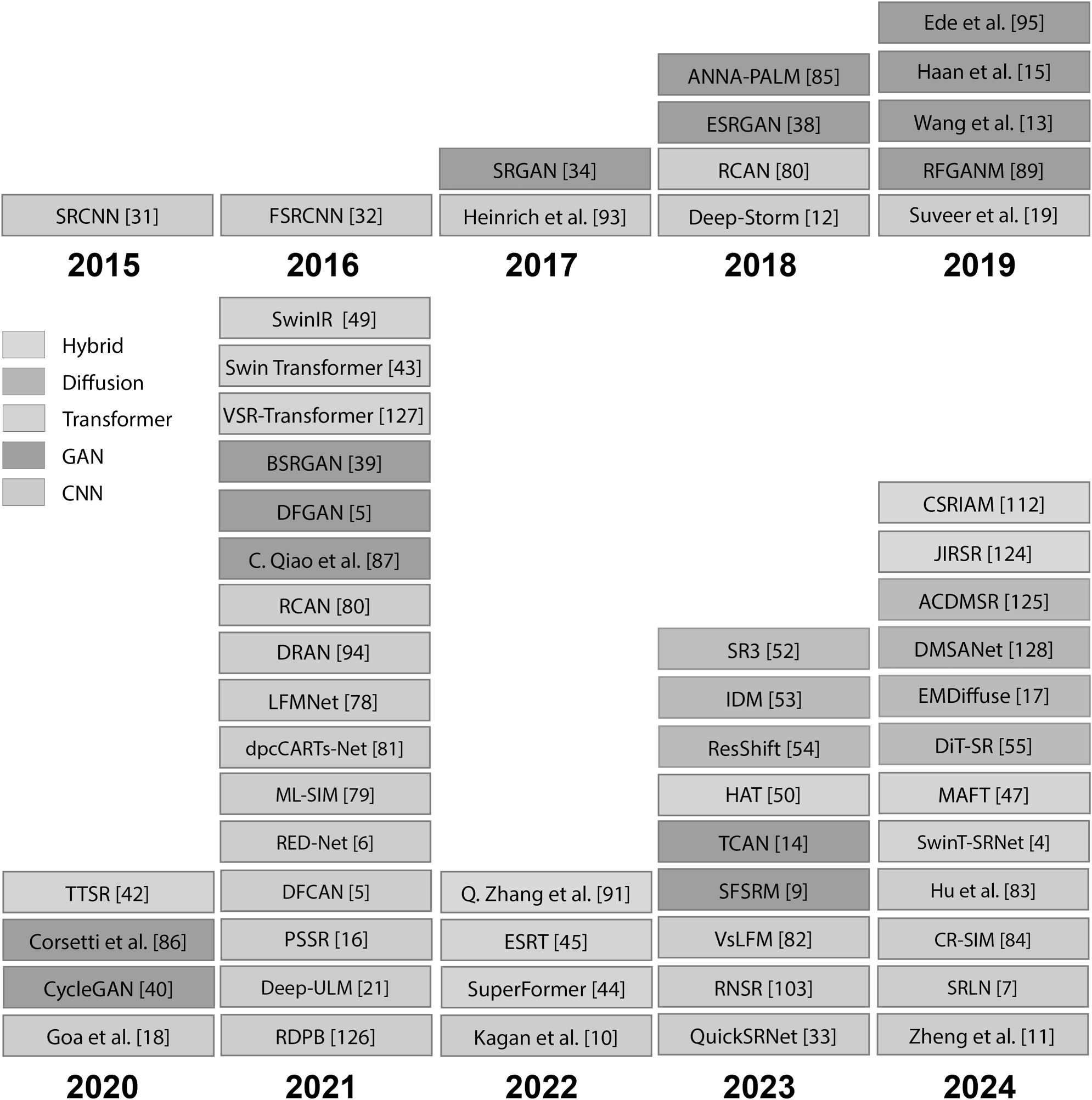
Deep learning super resolution methods by base architecture over time.
For the use in microscopy, the deep learning-based super resolution methods were first adopted only in 2018, while conventional super resolution microscopy was already established in the 1980s [12], [100]. The field of fluorescence microscopy was the first one to adopt it and remains a continuous driver for its development since [12]. SR was also quickly adopted in scanning electron microscopy just a year later in 2019, followed by light optical microscopy in 2021. Figure 27 show the adoption of SR for each type of microscopy over time.

Deep learning super resolution methods by imaging technique over time.
Up-/Downsampling: Basic upscaling methods include interpolation-based methods like bicubic interpolation and learnable methods such as transposed convolutions and sub-pixel convolutions [56]. While bicubic interpolation is computationally efficient, it often results in blurred images due to its non-adaptive nature and inability to preserve high-frequency details present in the original image [101]. To overcome the limitations of interpolation methods, learnable upscaling techniques have been integrated into neural networks [78], [88], [102]. Transposed convolutions expand the spatial dimensions of feature maps using learned kernels. They allow the network to perform upscaling in a data-driven manner, producing sharper and more detailed images [103]. However, transposed convolutions can introduce checkerboard artifacts caused by uneven overlap in the convolution process, and they are computationally more intensive than interpolation methods [104]. An alternative learnable method is the sub-pixel convolution, which rearranges elements from a low-resolution feature space into a high-resolution image through a process known as pixel shuffling [56], [89]. This increases the image resolution by performing most computations in the low-resolution space, thereby reducing computational load and memory usage. Sub-pixel convolution mitigates common artifacts associated with transposed convolutions and produces higher-quality results. Another common strategy involves simple upsampling techniques like nearest-neighbor or bilinear interpolation followed by convolutional layers that refine the upscaled image [104]. These methods are computationally inexpensive and easy to implement, but rely on subsequent convolutions to enhance image quality. Progressive upsampling methods, which incrementally increase image resolution in stages, allow the network to learn residuals at multiple scales. This can improve training stability and image quality by allowing gradual enhancement of image details [28]. Common downsampling techniques include pooling operations – such as max pooling [88], [102] and average pooling – and strided convolutions [78], [89]. Max pooling highlights prominent features but potentially discards fine details crucial for super resolution [105]. Average pooling, provides smoother feature representations but can lead to blurred outputs and loss of prominent images features [105]. Strided convolutions offer a learnable alternative by applying convolutional filters with strides, thus reducing spatial dimensions while maintaining trainable parameters in the downsampling process. This method allows the network to learn optimal downsampling kernels from data, potentially preserving more information than fixed pooling operations.
Attention mechanisms like Residual Channel Attention (RCA) [106], [107], [108] and Self-Calibrated Attention (SCA) [109] can be used to improve the overall super resolution results. These attention mechanisms can improve the feature extraction process within super resolution networks before the actual upsampling step. So, they do not perform upsampling or downsampling themselves but help enhancing the features that are upsampled to produce better HR images.
Geometric registration approach: Although geometric registration is crucial in the super resolution process, most reviewed publications did not explicitly report the registration approach or specific parameters used for image registration. An exception to this is the work of Suveer et al. [19]. They are using an image registration approach by Matuszewski et al. [110], combining the Harris point detector, log-polar magnitude point descriptor, and RANSAC to register TEM images. It has to be noted that outside of the microscopy context, image registration is sometimes directly integrated in the SR model. Examples of this are ShiftNet as part of the HighRes-net architecture by Deudon et al. [111] and RegNet as part of the DeepSUM architecture by Molini et al. [112]. This makes the image registration part of the end-to-end training process and enables adaptation to the domain-specific data.
Feature engineering and prior knowledge integration: Some papers report improved results when prior knowledge or precomputed additional features are integrated into the modelling process. For example, Chen et al. [9] could achieve increased robustness against noise in the input image by using a sub-pixel edge map which was added as an additional input channel. The edge map was computed based on the fluorophore’s radial symmetry and the local fluorescent signal intensity. The authors note that this method was used as conventional edge detection algorithms did not provide usable results as they do not consider diffraction effects that occur at the resolution limit of the imaging system [9]. Wenhan et al. [113] also use edge maps as an additional input, but make reconstruction of the HR edge maps part of the end-to-end training process as well, leading to sharper and more complete edges in the final HR image. Similar approaches have been reported for using the gradient profile as a prior, leading to a reduction in artifacts along edges in the super-resolved images [114]. As an extension to the edge-guided approaches, detail synthesis using exemplary HR images with similar image content was reported to enable higher quality SR results for high frequency details in the image, but with the drawback of the results being largely depended on the chosen example image [115]. Chen et al. [116] used conventional bicubic upscaling for increasing the image resolution before passing the input image to a diffusion model, thereby reducing the overall super resolution problem to a denoising problem that restores further details from the already super resolved image. If available for the specific use case, the integration of semantic priors from semantic segmentation models can also enhance SR results by enabling networks to learn specific reconstructions based on the semantic context of each image region [117].
Performance Metrics: Once of the most commonly used metrics in SR is PSNR, which is derived from MSE and quantifies pixelwise differences between the LR input and HR reconstruction. In addition, SSIM (or extension like MS-SSIM) is often used as it better represents more global image features like the overall structure and contrast, which brings closer to the human perception of image quality. To further account for perceptual quality, trainable methods derived from CNNs like LPIPS [62] are becoming more popular, as they capture these global / high level features even better. As an addition or in cases where ground truth / HR images are not available, reference-free metrics like NIQE [60] or BRISQUE [61] can be used to quantify image quality. [118].
If super resolution is applied to support a downstream task for which another model is applied (say image segmentation, object detection, etc.) task-based evaluation can be applied as an additional way to evaluate performance. For this, the change in the evaluation metric of the downstream model is observed to judge the SR model performance indirectly. [28].
Loss functions: Anagung et al. [119] compared different loss functions for super resolution individually. Euclidian loss was reported to be very sensitive so outliers, which makes it especially unfit for noisy data. Perceptual loss and DSSIM generally resulted in superior result visually. DSSIM, Charbonnier or MAE produced the best results in terms of evaluation metrics. [119]. For the pixel-based losses MAE and MSE, it can be noted that early models were mostly trained with MSE while more recent approaches mostly switched to MAE as it delivered better results due to lower sensitivity to outliers (noise) and less blurry reconstructions [120], [121]. When comparing perception-based loss functions, LPIPS [62] outperformed the conventional VGG-based loss in super resolution tasks [122]. Finding a good loss function for a specific use case is heavily depended on the training data and can hardly be broken down to a general recommendation. Combining different kinds of loss functions (for example a pixel-based loss like MAE and a loss function accounting for higher level features like DSSIM) and finding weights experimentally has to be proven as a successful approach, though, as those multi-component losses have been proven to achieve the best results [9], [123].
Datasets: An overview of publicly available as well as custom datasets is provided in Table 1. Where relevant information regarding dataset features, application domain, image size in pixels of the LR input images as well as the size of the HR output is provided. If further information about these datasets and work related to them is needed, this can be accessed via the source bibliography which is given in the reference column (Table 3).
Dataset summary table.
| Reference | Dataset | Application domain | Dataset size (# images) | LR | HR |
|---|---|---|---|---|---|
| B. Zu et al. [4] | POLLEN8BJ | Biology-microscopy | 9535 | Not specified | Not specified |
| POLLEN20L-det | Biology-microscopy | 7745 | Not specified | Not specified | |
| X. Zheng et al. [11] | DIV2K | General-microscopy | 6280 | 140×140 px | 560×560 px |
| G. Li et al. [124] | DIV2K | Other | Not specified | Not specified | Not specified |
| A. Niu et al. [125] | DIV2K | Other | 800 | Not specified | Not specified |
| C. N Christensen et al. [79] | DIV2K | General-microscopy | 1000 | Not specified | Not specified |
| X. Pu et al. [126] | DIV2K | Other | 800 | 50×50 px | Not specified |
| G. Li et al. [124] | Flickr2K | Other | 4744 | Not specified | Not specified |
| J. Cao et al. [127] | Vimeo-90K | Other | 4278 | Not specified | Not specified |
| C. Saharia et al. [52] | CelebA-HQ | Other | Not specified | 64×64 px | 512×512 px |
| Flickr-faces-HQ | Other | Not specified | 64×64 px | 256×256 px | |
| He et al. [128] | Cave | Geoscience | Not specified | Not specified | 512×512 px |
| Harvard | Geoscience | Not specified | Not specified | 512×512 px | |
| Chikusei | Geoscience | Not specified | Not specified | 512×512 px | |
| Bommanapally et al. [8] | LiveCell | Biology | 5239 | 256×256 px | 704×520 px |
| BioFilms | Biology | 7 | 256×256 px | 696×520 px | |
| C.elegans | Biology | 100 | 256×256 px | 1024×758 px | |
| Chen et al. [84] | BioSR | General | 10976 | 65 nm | Not specified |
| Song et al. [7] | BioSR | Biology-medicine | 20000 | 128×128 px | 256×256 px |
| Qiao et al. [5] | BioSR | Biology-microscopy | 20000 | 128×128 px | 256×256 px |
| Qiao et al. [87] | Custom | Biology-microscopy | 10000 | 64×64×9 voxels | 128×128×9 voxels |
| Lu et al. [82] | Custom | Biology-microscopy | 5000 | 25×25×169 px | 75×75×169 px |
| Durand et al. [129] | Custom | Biology-microscopy | Dataset-based | Not specified | 512×512 px |
| Zhang et al. [89] | Custom | Biomedicine-microscopy | Not specified | 96×96 px | 384×384 px. |
| Kagan et al. [10] | Custom | Photonics-microscopy | 1192 | 512×512 px | 2048×2048 px |
| Huang et al. [14] | Custom | Photonics-microscopy | 3000 | 256×256 px | 512×512 px |
| Gao et al. [18] | Custom | Biology-microscopy | 4000 | 200×200 px | 400×400 px |
| de Haan et al. [15] | Custom | Microscopy | 1920/4542 | 56.8 nm pixel size | 28.4 nm pixel size |
| Suveer et al. [19] | Custom | Microscopy | 871 | 512×512 px | 2048×2048 px |
5 Challenges and opportunities
Real-world data: Algorithms trained on synthetic data often fail to perform well on real-world data, despite excelling on synthetic test cases. This performance gap arises because real-world data is frequently affected by various distortions, including blur artifacts, sensor noise, quantization errors, varying resolutions, inconsistent lighting condition, among other factors. Unfortunately, real-world microscopy data is often sparse due to the significant challenges associated with its acquisition. Capturing high-quality data is time-consuming and expensive, particularly in scenarios where non-motorized microscopes require manual adjustments to meet specific acquisition requirements. Another major hurdle is geometric registration, which is essential for generating usable datasets for deep learning-based image super resolution. This process can be highly complex and, in some cases, impossible without specialized equipment. For instance, in life sciences where objects are often in motion, the acquisition system has to be equipped with multiple cameras to capture a scene with multiple resolutions at the same time. To address these challenges and improve the usability of real-world data, leveraging publicly available datasets can be a practical solution. These datasets can provide data for similar use cases, and techniques like transfer learning can help adapt models trained on existing data to new, specific applications. To make SR systems more robust against changing data resulting from different imaging conditions or samples, online learning approaches that finetune SR models continuously during use of the imaging system could be implemented. An example of this is shown by Wagner et al. [130] and their HyLFM approach, which constantly validates the reconstruction results against single HR slices and allows for finetuning or retraining in case certain evaluation metric thresholds are not met anymore.
Evaluation metrics: PSNR and SSIM are among the most widely used metrics for evaluating deep learning-based super resolution methods. However, PSNR, which is derived from the MSE, tends to favor overly smoothed images, making it less suitable for assessing methods aimed at enhancing image quality through super resolution. Both PSNR and SSIM are pixel-based metrics, which means they are unable to capture the perceptual quality of images effectively. Alternative metrics, such as LPIPS [62] and PieAPP [63], are designed to evaluate perceptual quality, but are trained on general-purpose datasets. As a result, their applicability to domain-specific data, such as microscopy images, is not guaranteed and may be limited. Evaluating the performance of trained deep learning-based super resolution methods in microscopy reliably remains a significant challenge and an open area of research in the field.
Loss functions: We provided a comprehensive overview of different loss functions used in the training of deep learning-based image super resolution methods, ranging from pixel-based loss functions to perceptual-based loss functions and custom-designed loss functions tailored for specific use cases. However, identifying a universally optimal loss function for a given application remains a challenge. This is largely due to the Perception-Distortion Tradeoff, which states that improving perceptual quality often comes at the expense of similarity between the model output and the training target [131]. For example, a model trained with MAE loss may achieve higher SSIM scores but lower LPIPS scores, whereas the same model trained with a perceptual-based loss function might show the opposite trend. Ultimately, selecting the right loss function depends on the specific requirements of the application and requires careful fine-tuning of loss function weighting. The best approach is to experiment with different weighted combinations of loss functions, evaluate every component’s impact, and choose the combination that produces the most satisfactory results in qualitative evaluation and/or based on improvement on a downstream image analysis task.
Architectures: Current challenges in deep learning-based image super resolution are to develop architectures that achieve a balance between high performance, efficiency, and adaptability. Generative Adversarial Networks (GANs) encounter stability problems, as the interaction of generator and discriminator often leads to unstable training. In addition, they are extremely computationally expensive because of their dual structure. Although diffusion models deliver photorealistic results, they struggle with inefficient computation and problems such as color shifts. Future trends indicate that mechanisms such as attention layers and residual layers will be increasingly integrated in order to optimize efficiency and feature extraction. In addition, modular and hierarchical approaches are gaining importance, including cascaded and multi-stage architectures, which can address complex challenges in real-world data more effectively. Moreover, research should focus on the development of smaller architectures that require less computing power and memory without significant performance degradation. At the same time, it is crucial to improve the theoretical understanding and interpretability of these “black-box” models in order to enable architectures tailored to the application.
Funding source: The European Union, the state of Baden-Württemberg, the Ostalbkreis and the city of Aalen.
Funding source: Aalen University of Applied Sciencs
Award Identifier / Grant number: Publication Fund
-
Research ethics: Not applicable.
-
Informed consent: Not applicable.
-
Author contributions: All authors have accepted responsibility for the entire content of this manuscript and approved its submission.
-
Use of Large Language Models, AI and Machine Learning Tools: Writefull Word-Add In for grammar and language checking.
-
Conflict of interests: The authors state no conflict of interest.
-
Research funding: The authors want to thank the European Union, the state of Baden-Württemberg, the Ostalbkreis and the city of Aalen for funding the SuReQA project as part of the “KI-Werkstatt Mittelstand”. Publication funded by Aalen University of Applied Sciences.
-
Data availability: Data sharing does not apply to this article as no datasets were generated or analyzed during the current study.
References
[1] S. W. Hell and J. Wichmann, “Breaking the diffraction resolution limit by stimulated emission: stimulated-emission-depletion fluorescence microscopy,” Opt. Lett., vol. 19, no. 11, 1994. https://doi.org/10.1364/ol.19.000780.Suche in Google Scholar PubMed
[2] M. G. Gustafsson, “Surpassing the lateral resolution limit by a factor of two using structured illumination microscopy,” J. Microsc., vol. 198, Pt. 2, pp. 82–87, 2000, https://doi.org/10.1046/j.1365-2818.2000.00710.x.Suche in Google Scholar PubMed
[3] M. J. Rust, M. Bates, and X. Zhuang, “Sub-diffraction-limit imaging by stochastic optical reconstruction microscopy (STORM),” Nat. Methods, vol. 3, no. 10, pp. 793–795, 2006, https://doi.org/10.1038/nmeth929.Suche in Google Scholar PubMed PubMed Central
[4] B. Zu, T. Cao, Y. Li, J. Li, F. Ju, and H. Wang, “SwinT-SRNet: Swin transformer with image super-resolution reconstruction network for pollen images classification,” Eng. Appl. Artif. Intell., vol. 133, p. 108041, 2024, https://doi.org/10.1016/j.engappai.2024.108041.Suche in Google Scholar
[5] C. Qiao, et al.., “Evaluation and development of deep neural networks for image super-resolution in optical microscopy,” Nat. Methods, vol. 18, no. 2, pp. 194–202, 2021, https://doi.org/10.1038/s41592-020-01048-5.Suche in Google Scholar PubMed
[6] Z. H. Shah, et al.., “Deep-learning based denoising and reconstruction of super-resolution structured illumination microscopy images,” Photon. Res., vol. 9, no. 5, p. B168, 2021, https://doi.org/10.1364/PRJ.416437.Suche in Google Scholar
[7] L. Song, et al.., “Super-resolution reconstruction of structured illumination microscopy using deep-learning and sparse deconvolution,” Opt Laser. Eng., vol. 174, p. 107968, 2024, https://doi.org/10.1016/j.optlaseng.2023.107968.Suche in Google Scholar
[8] V. Bommanapally, D. Abeyrathna, P. Chundi, and M. Subramaniam, “Super resolution-based methodology for self-supervised segmentation of microscopy images,” Front. Microbiol., vol. 15, p. 1255850, 2024, https://doi.org/10.3389/fmicb.2024.1255850.Suche in Google Scholar PubMed PubMed Central
[9] R. Chen, et al.., “Single-frame deep-learning super-resolution microscopy for intracellular dynamics imaging,” Nat. Commun., vol. 14, no. 1, p. 2854, 2023, https://doi.org/10.1038/s41467-023-38452-2.Suche in Google Scholar PubMed PubMed Central
[10] B. Kagan, A. Hendler-Neumark, V. Wulf, D. Kamber, R. Ehrlich, and G. Bisker, “Super-resolution near-infrared fluorescence microscopy of single-walled carbon nanotubes using deep learning,” Adv. Photon. Res., vol. 3, no. 11, 2022, https://doi.org/10.1002/adpr.202200244.Suche in Google Scholar
[11] X. Zheng, et al.., “Deep learning enhanced super-resolution x-ray fluorescence microscopy by a dual-branch network,” Optica, vol. 11, no. 2, p. 146, 2024, https://doi.org/10.1364/OPTICA.503398.Suche in Google Scholar
[12] E. Nehme, L. E. Weiss, T. Michaeli, and Y. Shechtman, “Deep-STORM: super-resolution single-molecule microscopy by deep learning,” Optica, vol. 5, no. 4, p. 458, 2018, https://doi.org/10.1364/OPTICA.5.000458.Suche in Google Scholar
[13] H. Wang, et al.., “Deep learning enables cross-modality super-resolution in fluorescence microscopy,” Nat. Methods, vol. 16, no. 1, pp. 103–110, 2019, https://doi.org/10.1038/s41592-018-0239-0.Suche in Google Scholar PubMed PubMed Central
[14] B. Huang, et al.., “Enhancing image resolution of confocal fluorescence microscopy with deep learning,” PhotoniX, vol. 4, no. 1, 2023, https://doi.org/10.1186/s43074-022-00077-x.Suche in Google Scholar
[15] K. de Haan, Z. S. Ballard, Y. Rivenson, Y. Wu, and A. Ozcan, “Resolution enhancement in scanning electron microscopy using deep learning,” Sci. Rep., vol. 9, no. 1, p. 12050, 2019, https://doi.org/10.1038/s41598-019-48444-2.Suche in Google Scholar PubMed PubMed Central
[16] L. Fang, et al.., “Deep learning-based point-scanning super-resolution imaging,” Nat. Methods, vol. 18, no. 4, pp. 406–16, 2021, https://doi.org/10.1038/s41592-021-01080-z.Suche in Google Scholar PubMed PubMed Central
[17] C. Lu, et al.., “Diffusion-based deep learning method for augmenting ultrastructural imaging and volume electron microscopy,” Nat. Commun., vol. 15, no. 1, p. 4677, 2024, https://doi.org/10.1038/s41467-024-49125-z.Suche in Google Scholar PubMed PubMed Central
[18] Z. Gao, W. Ma, S. Huang, P. Hua, and C. Lan, “Deep learning for super-resolution in a field emission scanning electron microscope,” AI, vol. 1, no. 1, pp. 1–10, 2020, https://doi.org/10.3390/ai1010001.Suche in Google Scholar
[19] A. Suveer, A. Gupta, G. Kylberg, and I.-M. Sintorn, “Super-resolution reconstruction of transmission electron microscopy images using deep learning,” in 2019 IEEE 16th International Symposium on Biomedical Imaging (ISBI 2019), Venice, Italy, IEEE, 2019, pp. 548–51.10.1109/ISBI.2019.8759153Suche in Google Scholar
[20] S. Aymaz and C. Köse, “A novel image decomposition-based hybrid technique with super-resolution method for multi-focus image fusion,” Inf. Fusion, vol. 45, pp. 113–27, 2019, https://doi.org/10.1016/j.inffus.2018.01.015.Suche in Google Scholar
[21] R. J. G. van Sloun, et al.., “Super-resolution ultrasound localization microscopy through deep learning,” IEEE Trans. Med. Imag., vol. 40, no. 3, pp. 829–839, 2021, https://doi.org/10.1109/TMI.2020.3037790.Suche in Google Scholar PubMed
[22] T. Yang, Y. Luo, W. Ji, and G. Yang, “Advancing biological super-resolution microscopy through deep learning: a brief review,” Biophy. Rep., vol. 7, no. 4, pp. 253–266, 2021, https://doi.org/10.52601/bpr.2021.210019.Suche in Google Scholar PubMed PubMed Central
[23] W. Yang, X. Zhang, Y. Tian, W. Wang, J.-H. Xue, and Q. Liao, “Deep learning for single image super-resolution: A brief review,” IEEE Trans. Multimedia, vol. 21, no. 12, pp. 3106–3121, 2019, https://doi.org/10.1109/TMM.2019.2919431.Suche in Google Scholar
[24] S. Anwar, S. Khan, and N. Barnes, “A deep journey into super-resolution: A survey,” 2019. [Online]. Available: http://arxiv.org/pdf/1904.07523v3.Suche in Google Scholar
[25] H. Chen, X. He, L. Qing, Y. Wu, C. Ren, and C. Zhu, “Real-world single image super-resolution: A brief review,” 2021. [Online]. Available: http://arxiv.org/pdf/2103.02368v1.Suche in Google Scholar
[26] A. Liu, Y. Liu, J. Gu, Y. Qiao, and C. Dong, “Blind image super-resolution: A survey and beyond,” 2021. [Online]. Available: http://arxiv.org/pdf/2107.03055v1.10.1109/TPAMI.2022.3203009Suche in Google Scholar PubMed
[27] C. Tian, X. Zhang, J. C.-W. Lin, W. Zuo, Y. Zhang, and C.-W. Lin, “Generative adversarial networks for image super-resolution: A survey,” 2022. [Online]. Available: http://arxiv.org/pdf/2204.13620v2.Suche in Google Scholar
[28] B. B. Moser, F. Raue, S. Frolov, S. Palacio, J. Hees, and A. Dengel, “Hitchhiker’s guide to super-resolution: Introduction and recent advances,” IEEE Trans. Pattern Anal. Mach. Intell., vol. 45, no. 8, pp. 9862–9882, 2023, https://doi.org/10.1109/TPAMI.2023.3243794.Suche in Google Scholar PubMed
[29] B. B. Moser, A. S. Shanbhag, F. Raue, S. Frolov, S. Palacio, and A. Dengel, “Diffusion models, image super-resolution and everything: A survey,” IEEE Trans. Neural Netw. Learning Syst., pp. 1–21, 2024, https://doi.org/10.1109/TNNLS.2024.3476671.Suche in Google Scholar PubMed
[30] E. N. Ward, A. Scheeder, M. Barysevich, and C. F. Kaminski, “Self-driving microscopes: AI meets super-resolution microscopy,” Small Methods, p. e2401757, 2025, https://doi.org/10.1002/smtd.202401757.Suche in Google Scholar PubMed
[31] C. Dong, C. C. Loy, K. He, and X. Tang, “Image super-resolution using deep convolutional networks,” 2014. [Online]. Available: http://arxiv.org/pdf/1501.00092v3.Suche in Google Scholar
[32] C. Dong, C. C. Loy, and X. Tang, “Accelerating the super-resolution convolutional neural network,” 2016. [Online]. Available: http://arxiv.org/pdf/1608.00367v1.Suche in Google Scholar
[33] G. Berger, M. Dhingra, A. Mercier, Y. Savani, S. Panchal, and F. Porikli, “QuickSRNet: Plain single-image super-resolution architecture for faster inference on mobile platforms,” 2023. [Online]. Available: http://arxiv.org/pdf/2303.04336v2.10.1109/CVPRW59228.2023.00212Suche in Google Scholar
[34] C. Ledig, et al.., “Photo-realistic single image super-resolution using a generative adversarial network,” 2016. [Online]. Available: http://arxiv.org/pdf/1609.04802v5.Suche in Google Scholar
[35] M. Bevilacqua, A. Roumy, C. Guillemot, and M. A. Morel, “Low-complexity single-image low-complexity single-image super-resolution based on nonnegative neighbor embedding,” in British Machine Vision Conference, Surrey, BMVA Press, 2012.10.5244/C.26.135Suche in Google Scholar
[36] R. Zeyde, M. Elad, and M. Protter, “On single image scale-up using sparse-representations,” in Lecture Notes in Computer Science, Curves and Surfaces, J.-D. Boissonnat, Ed., Berlin, Heidelberg, Springer Berlin Heidelberg, 2012, pp. 711–730.10.1007/978-3-642-27413-8_47Suche in Google Scholar
[37] D. Martin, C. Fowlkes, D. Tal, and J. Malik, “A database of human segmented natural images and its application to evaluating segmentation algorithms and measuring ecological statistics,” in Proceedings Eighth IEEE International Conference on Computer Vision. ICCV 2001, Vancouver, BC, Canada, IEEE, 2001, pp. 416–423.10.1109/ICCV.2001.937655Suche in Google Scholar
[38] X. Wang, et al.., “ESRGAN: Enhanced super-resolution generative adversarial networks,” 2018. [Online]. Available: http://arxiv.org/pdf/1809.00219v2.Suche in Google Scholar
[39] K. Zhang, J. Liang, L. van Gool, and R. Timofte, “Designing a practical degradation model for deep blind image super-resolution,” 2021. [Online]. Available: http://arxiv.org/pdf/2103.14006v2.10.1109/ICCV48922.2021.00475Suche in Google Scholar
[40] J.-Y. Zhu, T. Park, P. Isola, and A. A. Efros, “Unpaired Image-to-image translation using cycle-consistent adversarial networks,” 2017. [Online]. Available: http://arxiv.org/pdf/1703.10593v7.10.1109/ICCV.2017.244Suche in Google Scholar
[41] M. Mirza and S. Osindero, “Conditional generative adversarial nets,” 2014. [Online]. Available: http://arxiv.org/pdf/1411.1784v1.Suche in Google Scholar
[42] F. Yang, H. Yang, J. Fu, H. Lu, and B. Guo, “Learning texture transformer network for image super-resolution,” in 2020 IEEE/CVF Conference on Computer Vision and Pattern Recognition (CVPR), 2020, pp. 5790–5799. https://doi.org/10.1109/cvpr42600.2020.00583.Suche in Google Scholar
[43] Z. Liu, et al.., “Swin transformer: Hierarchical vision transformer using shifted windows,” 2021. [Online]. Available: http://arxiv.org/pdf/2103.14030v2.Suche in Google Scholar
[44] C. Forigua, M. Escobar, and P. Arbelaez, “SuperFormer: volumetric transformer architectures for mri super-resolution,” vol. 13570, no. 1, pp. 132–141, 2022, https://doi.org/10.1007/978-3-031-16980-9_13.Suche in Google Scholar
[45] Z. Lu, J. Li, H. Liu, C. Huang, L. Zhang, and T. Zeng, “Transformer for single image super-resolution,” 2021. [Online]. Available: http://arxiv.org/pdf/2108.11084v3.Suche in Google Scholar
[46] A. Vaswani, et al.., “Attention is all you need,” 2017. [Online]. Available: http://arxiv.org/pdf/1706.03762v7.Suche in Google Scholar
[47] G. Li, Z. Cui, M. Li, Y. Han, and T. Li, “Multi-attention fusion transformer for single-image super-resolution,” Sci. Rep., vol. 14, no. 1, p. 10222, 2024, https://doi.org/10.1038/s41598-024-60579-5.Suche in Google Scholar PubMed PubMed Central
[48] J.-B. Huang, A. Singh, and N. Ahuja, “Single image super-resolution from transformed self-exemplars,” in 2015 IEEE Conference on Computer Vision and Pattern Recognition (CVPR), Boston, MA, USA, IEEE, 2015, pp. 5197–5206.10.1109/CVPR.2015.7299156Suche in Google Scholar
[49] J. Liang, J. Cao, G. Sun, K. Zhang, L. van Gool, and R. Timofte, “SwinIR: image restoration using swin transformer,” in 2021 IEEE/CVF International Conference on Computer Vision Workshops (ICCVW), Montreal, BC, Canada, IEEE, 2021, pp. 1833–1844.10.1109/ICCVW54120.2021.00210Suche in Google Scholar
[50] X. Chen, et al.., “HAT: hybrid attention transformer for image restoration,” 2023. [Online]. Available: http://arxiv.org/pdf/2309.05239v2.Suche in Google Scholar
[51] R. Rombach, A. Blattmann, D. Lorenz, P. Esser, and B. Ommer, “High-resolution image synthesis with latent diffusion models,” 2021. [Online]. Available: http://arxiv.org/pdf/2112.10752v2.Suche in Google Scholar
[52] C. Saharia, J. Ho, W. Chan, T. Salimans, D. J. Fleet, and M. Norouzi, “Image super-resolution via iterative refinement,” IEEE Trans. Pattern Anal. Mach. Intell., vol. 45, no. 4, pp. 4713–4726, 2023, https://doi.org/10.1109/TPAMI.2022.3204461.Suche in Google Scholar PubMed
[53] S. Gao, et al.., “Implicit Diffusion Models for Continuous Super-Resolution,” 2023. [Online]. Available: http://arxiv.org/pdf/2303.16491v2.Suche in Google Scholar
[54] Z. Yue, J. Wang, and C. C. Loy, “ResShift: Efficient diffusion model for image super-resolution by residual shifting,” 2023. [Online]. Available: http://arxiv.org/pdf/2307.12348v3.Suche in Google Scholar
[55] K. Cheng, et al.., “Effective diffusion transformer architecture for image super-resolution,” 2024. [Online]. Available: http://arxiv.org/pdf/2409.19589v1.Suche in Google Scholar
[56] W. Shi, et al.., “Real-time single image and video super-resolution using an efficient sub-pixel convolutional neural network,” in 2016 IEEE Conference on Computer Vision and Pattern Recognition (CVPR), Las Vegas, NV, USA, IEEE, 2016, pp. 1874–83.10.1109/CVPR.2016.207Suche in Google Scholar
[57] X. Hu, H. Mu, X. Zhang, Z. Wang, T. Tan, and J. Sun, “Meta-SR: A magnification-arbitrary network for super-resolution,” 2019. [Online]. Available: http://arxiv.org/pdf/1903.00875v4.Suche in Google Scholar
[58] K. Simonyan and A. Zisserman, “Very Deep Convolutional Networks for Large-Scale Image Recognition,” 2014. [Online]. Available: http://arxiv.org/pdf/1409.1556v6.Suche in Google Scholar
[59] V. N, P. D, M. C. Bh, S. S. Channappayya, and S. S. Medasani, “Blind image quality evaluation using perception based features,” in 2015 Twenty First National Conference on Communications (NCC), Mumbai, India, 2015, pp. 1–6.10.1109/NCC.2015.7084843Suche in Google Scholar
[60] A. Mittal, R. Soundararajan, and A. C. Bovik, “Making a “Completely Blind” image quality analyzer,” IEEE Signal Process. Lett., vol. 20, no. 3, pp. 209–212, 2013, https://doi.org/10.1109/LSP.2012.2227726.Suche in Google Scholar
[61] A. Mittal, A. K. Moorthy, and A. C. Bovik, “Blind/referenceless image spatial quality evaluator,” in 2011 Conference Record of the Forty Fifth Asilomar Conference on Signals, Systems and Computers (ASILOMAR), Pacific Grove, CA, USA, IEEE, 2011, pp. 723–727.10.1109/ACSSC.2011.6190099Suche in Google Scholar
[62] R. Zhang, P. Isola, A. A. Efros, E. Shechtman, and O. Wang, “The unreasonable effectiveness of deep features as a perceptual metric,” 2018. [Online]. Available: http://arxiv.org/pdf/1801.03924.10.1109/CVPR.2018.00068Suche in Google Scholar
[63] E. Prashnani, H. Cai, Y. Mostofi, and P. Sen, PieAPP: Perceptual Image-Error Assessment through Pairwise Preference, E. Prashnani, [Online]. Available: http://arxiv.org/pdf/1806.02067.Suche in Google Scholar
[64] Y. Li, M. Chen, K. Wang, J. Ma, A. C. Bovik, and Y. Zhang, “SAMScore: A content structural similarity metric for image translation evaluation,” 2023. [Online]. Available: http://arxiv.org/pdf/2305.15367v2.Suche in Google Scholar
[65] M. Heusel, H. Ramsauer, T. Unterthiner, B. Nessler, and S. Hochreiter, “GANs trained by a two time-scale update rule converge to a local nash equilibrium,” [Online]. Available: http://arxiv.org/pdf/1706.08500v6.Suche in Google Scholar
[66] Z. Liu, et al.., “A survey on applications of deep learning in microscopy image analysis,” Comput. Biol. Med., vol. 134, p. 104523, 2021, https://doi.org/10.1016/j.compbiomed.2021.104523.Suche in Google Scholar PubMed
[67] R. B. A. Canette, “MICROSCOPY | confocal laser scanning microscopy,” in Encyclopedia of Food Microbiology, 2nd ed., 2014, pp. 676–83.10.1016/B978-0-12-384730-0.00214-7Suche in Google Scholar
[68] J. Enderlein, “4.09 – Advanced fluorescence microscopy,” Comprehensive Biomedical Physics, pp. 111–151, 2014, [Online]. Available: https://doi.org/10.1016/B978-0-444-53632-7.00409-3.Suche in Google Scholar
[69] V. Mennella, “Structured illumination microscopy,” in Encyclopedia of Cell Biology, Elsevier, 2016, pp. 86–98.10.1016/B978-0-12-394447-4.20093-XSuche in Google Scholar
[70] Z. Zhang, L. Cong, L. Bai, and K. Wang, “Light-field microscopy for fast volumetric brain imaging,” J. Neurosci. Methods, vol. 352, p. 109083, 2021, https://doi.org/10.1016/j.jneumeth.2021.109083.Suche in Google Scholar PubMed
[71] G. Wang and N. Fang, “Detecting and tracking nonfluorescent nanoparticle probes in live cells,” Methods Enzymol., vol. 504, pp. 83–108, 2012, https://doi.org/10.1016/B978-0-12-391857-4.00004-5.Suche in Google Scholar PubMed
[72] J. D. Tucker, A. C. Seña, P. Frederick Sparling, X.-S. Chen, and M. S. Cohen, “Treponemal infections,” in Tropical Infectious Diseases: Principles, Pathogens and Practice, Elsevier, 2011, pp. 289–294.10.1016/B978-0-7020-3935-5.00043-4Suche in Google Scholar
[73] J. W. J. H. Holgate, “Light microscopy and histochemical methods scanning electron microscopy transmission electron microscopy image analysis: light microscopy and histochemical methods,” in Encyclopedia of Food Sciences and Nutrition, 2nd ed., 2003, pp. 3917–3922.10.1016/B0-12-227055-X/00778-1Suche in Google Scholar
[74] M. Ovesný, P. Křížek, J. Borkovec, Z. Svindrych, and G. M. Hagen, “ThunderSTORM: a comprehensive ImageJ plug-in for PALM and STORM data analysis and super-resolution imaging,” Bioinformatics (Oxford, England), vol. 30, no. 16, pp. 2389–2390, 2014, https://doi.org/10.1093/bioinformatics/btu202.Suche in Google Scholar PubMed PubMed Central
[75] C. T. Rueden, et al.., “ImageJ2: ImageJ for the next generation of scientific image data,” BMC Bioinformatics, vol. 18, no. 1, p. 529, 2017, https://doi.org/10.1186/s12859-017-1934-z.Suche in Google Scholar PubMed PubMed Central
[76] J. Schindelin, et al.., “Fiji: an open-source platform for biological-image analysis,” Nat. Methods, vol. 9, no. 7, pp. 676–682, 2012, https://doi.org/10.1038/nmeth.2019.Suche in Google Scholar PubMed PubMed Central
[77] S. Gazagnes, E. Soubies, and L. Blanc-Féraud, “High density molecule localization for super-resolution microscopy using CEL0 based sparse approximation,” in IEEE International Symposium on Biomedical Imaging (ISBI), 2017, p. 4.10.1109/ISBI.2017.7950460Suche in Google Scholar
[78] J. P. Vizcaíno, F. Saltarin, Y. Belyaev, R. Lyck, T. Lasser, and P. Favaro, “Learning to reconstruct confocal microscopy stacks from single light field images,” IEEE Trans. Comput. Imaging, vol. 7, pp. 775–788, 2021, https://doi.org/10.1109/TCI.2021.3097611.Suche in Google Scholar
[79] C. N. Christensen, E. N. Ward, M. Lu, P. Lio, and C. F. Kaminski, “ML-SIM: universal reconstruction of structured illumination microscopy images using transfer learning,” Biomed. Opt. Express, vol. 12, no. 5, pp. 2720–2733, 2021, https://doi.org/10.1364/BOE.414680.Suche in Google Scholar PubMed PubMed Central
[80] Y. Zhang, K. Li, K. Li, L. Wang, B. Zhong, and Y. Fu, “Image Super-Resolution Using Very Deep Residual Channel Attention Networks,” 2018. [Online]. Available: http://arxiv.org/pdf/1807.02758v2.Suche in Google Scholar
[81] Z. Wang, D. Zhang, N. Wang, and J. He, “Surpassing the diffraction limit using an external aperture modulation subsystem and related deep learning method,” Opt. Express, vol. 29, no. 20, pp. 31099–31114, 2021, https://doi.org/10.1364/OE.432507.Suche in Google Scholar PubMed
[82] Z. Lu, et al.., “Virtual-scanning light-field microscopy for robust snapshot high-resolution volumetric imaging,” Nat. Methods, vol. 20, no. 5, pp. 735–746, 2023, https://doi.org/10.1038/s41592-023-01839-6.Suche in Google Scholar PubMed PubMed Central
[83] X. Hu, et al.., “Deep-learning-augmented microscopy for super-resolution imaging of nanoparticles,” Opt. Express, vol. 32, no. 1, pp. 879–890, 2024, https://doi.org/10.1364/OE.505060.Suche in Google Scholar PubMed
[84] Y. Chen, et al.., “Deep learning enables contrast-robust super-resolution reconstruction in structured illumination microscopy,” Opt. Express, vol. 32, no. 3, pp. 3316–3328, 2024, https://doi.org/10.1364/OE.507017.Suche in Google Scholar PubMed
[85] W. Ouyang, A. Aristov, M. Lelek, X. Hao, and C. Zimmer, “Deep learning massively accelerates super-resolution localization microscopy,” Nat. Biotechnol., vol. 36, no. 5, pp. 460–468, 2018, https://doi.org/10.1038/nbt.4106.Suche in Google Scholar PubMed
[86] S. Corsetti, et al.., “Widefield light sheet microscopy using an Airy beam combined with deep-learning super-resolution,” OSA Continuum, vol. 3, no. 4, p. 1068, 2020, https://doi.org/10.1364/OSAC.391644.Suche in Google Scholar
[87] C. Qiao, et al.., “3D structured illumination microscopy via channel attention generative adversarial network,” IEEE J. Select. Topics Quantum Electron., vol. 27, no. 4, pp. 1–11, 2021, https://doi.org/10.1109/JSTQE.2021.3060762.Suche in Google Scholar
[88] H. Park, et al.., “Deep learning enables reference-free isotropic super-resolution for volumetric fluorescence microscopy,” Nat. Commun., vol. 13, no. 1, p. 3297, 2022, https://doi.org/10.1038/s41467-022-30949-6.Suche in Google Scholar PubMed PubMed Central
[89] H. Zhang, et al.., “High-throughput, high-resolution deep learning microscopy based on registration-free generative adversarial network,” Biomed. Opt. Express, vol. 10, no. 3, pp. 1044–1063, 2019, https://doi.org/10.1364/BOE.10.001044.Suche in Google Scholar PubMed PubMed Central
[90] Z. Lu, J. Li, H. Liu, C. Huang, L. Zhang, and T. Zeng, “Transformer for single image super-resolution,” in Proceedings of the IEEE/CVF Conference on Computer Vision and Pattern Recognition (CVPR) Workshops, 2022, pp. 457–466.10.1109/CVPRW56347.2022.00061Suche in Google Scholar
[91] Q. Zhang, et al.., “Deep learning-based single-shot structured illumination microscopy,” Opt Laser. Eng., vol. 155, p. 107066, 2022, https://doi.org/10.1016/j.optlaseng.2022.107066.Suche in Google Scholar
[92] W.-S. Ryu, Molecular Virology of Human Pathogenic Viruses, vol. 2, Cambridge, Academic press, 2017, pp. 21–29.10.1016/B978-0-12-800838-6.00002-3Suche in Google Scholar
[93] L. Heinrich, J. A. Bogovic, and S. Saalfeld, “Deep learning for isotropic super-resolution from non-isotropic 3D electron microscopy,” 2017. [Online]. Available: http://arxiv.org/pdf/1706.03142v1.10.1007/978-3-319-66185-8_16Suche in Google Scholar
[94] J. Wang, C. Lan, C. Wang, and Z. Gao, “Deep learning super-resolution electron microscopy based on deep residual attention network,” Int. J. Imaging Syst. Tech., vol. 31, no. 4, pp. 2158–2169, 2021, https://doi.org/10.1002/ima.22588.Suche in Google Scholar
[95] J. M. Ede, “Deep learning supersampled scanning transmission electron microscopy,” 2019. [Online]. Available: http://arxiv.org/pdf/1910.10467v2.Suche in Google Scholar
[96] C. Dong, C. C. Loy, K. He, and X. Tang, “Learning a deep convolutional network for image super-resolution,” in Lecture Notes in Computer Science, Computer Vision – ECCV 2014, D. Fleet, T. Pajdla, B. Schiele, and T. Tuytelaars, Eds., Cham, Springer International Publishing, 2014, pp. 184–199.10.1007/978-3-319-10593-2_13Suche in Google Scholar
[97] C. Dong, C. C. Loy, and X. Tang, “Accelerating the super-resolution convolutional neural network,” in Lecture Notes in Computer Science, Computer Vision – ECCV 2016, B. Leibe, J. Matas, N. Sebe, and M. Welling, Eds., Cham: Springer International Publishing, 2016, pp. 391–407.10.1007/978-3-319-46475-6_25Suche in Google Scholar
[98] I. Goodfellow, et al.., “Generative adversarial nets,” in Advances in Neural Information Processing Systems, 2014. [Online]. Available: https://proceedings.neurips.cc/paper_files/paper/2014/file/5ca3e9b122f61f8f06494c97b1afccf3-Paper.pdf.Suche in Google Scholar
[99] J. Ho, A. Jain, and P. Abbeel, “Denoising diffusion probabilistic models,” 2020. [Online]. Available: http://arxiv.org/pdf/2006.11239v2.Suche in Google Scholar
[100] M. Weigert, et al.., “Content-aware image restoration: pushing the limits of fluorescence microscopy,” Nat. Methods, vol. 15, no. 12, pp. 1090–1097, 2018, https://doi.org/10.1038/s41592-018-0216-7.Suche in Google Scholar PubMed
[101] M. Jahnavi, D. R. Rao, and A. Sujatha, “A comparative study of super-resolution interpolation techniques: Insights for selecting the most appropriate method,” Procedia Comput. Sci., vol. 233, pp. 504–517, 2024, https://doi.org/10.1016/j.procs.2024.03.240.Suche in Google Scholar
[102] J. Liao, J. Qu, Y. Hao, and J. Li, “Deep-learning-based methods for super-resolution fluorescence microscopy,” J. Innov. Opt. Health Sci., vol. 16, no. 03, 2023, https://doi.org/10.1142/S1793545822300166.Suche in Google Scholar
[103] W.-S. Lai, J.-B. Huang, N. Ahuja, and M.-H. Yang, “Deep Laplacian Pyramid Networks for Fast and Accurate Super-Resolution,” in 2017 IEEE conference on computer vision and pattern recognition (CVPR), Honolulu, HI, IEEE, 2017, pp. 5835–5843.10.1109/CVPR.2017.618Suche in Google Scholar
[104] A. Odena, V. Dumoulin, and C. Olah, “Deconvolution and checkerboard artifacts,” Distill, vol. 1, no. 10, 2016, https://doi.org/10.23915/distill.00003.Suche in Google Scholar
[105] A. Zafar, et al.., “A comparison of pooling methods for convolutional neural networks,” Appl. Sci., vol. 12, no. 17, p. 8643, 2022, https://doi.org/10.3390/app12178643.Suche in Google Scholar
[106] J. Cai, Z. Meng, and C. M. Ho, “Residual channel attention generative adversarial network for image super-resolution and noise reduction,” 2020. [Online]. Available: http://arxiv.org/pdf/2004.13674.10.1109/CVPRW50498.2020.00235Suche in Google Scholar
[107] S. Karthick and N. Muthukumaran, “Deep regression network for single-image super-resolution based on down- and upsampling with RCA blocks,” National Academy Science Letters, vol. 47, no. 3, pp. 279–283, 2024, https://doi.org/10.1007/s40009-023-01353-5.Suche in Google Scholar
[108] Y. Zhang, K. Li, K. Li, L. Wang, B. Zhong, and Y. Fu, “Image super-resolution using very deep residual channel attention networks,” 2018. [Online]. Available: http://arxiv.org/pdf/1807.02758.10.1007/978-3-030-01234-2_18Suche in Google Scholar
[109] K. Cheng and C. Wu, “Self-calibrated attention neural network for real-world super resolution,” pp. 453–467, 2020. [Online]. Available: https://link.springer.com/chapter/10.1007/978-3-030-67070-2_27.10.1007/978-3-030-67070-2_27Suche in Google Scholar
[110] D. J. Matuszewski, A. Hast, C. Wählby, and I.-M. Sintorn, “A short feature vector for image matching: The Log-Polar Magnitude feature descriptor,” PLoS One, vol. 12, no. 11, p. e0188496, 2017, https://doi.org/10.1371/journal.pone.0188496.Suche in Google Scholar PubMed PubMed Central
[111] M. Deudon, et al.., “HighRes-net: Recursive fusion for multi-frame super-resolution of satellite imagery,” 2020.Suche in Google Scholar
[112] A. Bordone Molini, D. Valsesia, G. Fracastoro, and E. Magli, “DeepSUM: Deep neural network for super-resolution of unregistered multitemporal images,” IEEE Trans. Geosci. Remote Sensing, vol. 58, no. 5, pp. 3644–3656, 2020, https://doi.org/10.1109/TGRS.2019.2959248.Suche in Google Scholar
[113] Y. Wenhan, et al.., “Deep edge guided recurrent residual learning for image super-resolution,” IEEE Trans. Image Process.: Publication IEEE Signal Process. Soc., vol. 26, no. 12, pp. 5895–5907, 2017, https://doi.org/10.1109/TIP.2017.2750403.Suche in Google Scholar PubMed
[114] J. Sun, Z. Xu, and H-Y. Shum, Image Super-Resolution using Gradient Profile Prior, Computer Vision and Pattern Recognition, 2008.Suche in Google Scholar
[115] Y. Tai, S. Liu, M. S. Brown, and S. Lin, “Super resolution using edge prior and single image detail synthesis,” in IEEE Computer Society Conference on Computer Vision and Pattern Recognition, San Francisco, IEEE, 2010.10.1109/CVPR.2010.5539933Suche in Google Scholar
[116] J. Chen, L. Jia, J. Zhang, Y. Feng, X. Zhao, and R. Tao, “Super-resolution for land surface temperature retrieval images via cross-scale diffusion model using reference images,” Remote Sensing, vol. 16, no. 8, p. 1356, 2024, https://doi.org/10.3390/rs16081356.Suche in Google Scholar
[117] X. Wang, K. Yu, C. Dong, and C. C. Loy, “Recovering realistic texture in image super-resolution by deep spatial feature transform,” 2018. [Online]. Available: http://arxiv.org/pdf/1804.02815.10.1109/CVPR.2018.00070Suche in Google Scholar
[118] M. Arabboev, S. Begmatov, M. Rikhsivoev, K. Nosirov, and S. Saydiakbarov, “Comprehensive review of image super-resolution metrics: classical and AI-based approaches,” Acta IMEKO, vol. 13, no. 1, pp. 1–8, 2024, https://doi.org/10.21014/actaimeko.v13i1.1679.Suche in Google Scholar
[119] Y. Anagun, S. Isik, and E. Seke, “SRLibrary: Comparing different loss functions for super-resolution over various convolutional architectures,” J. Vis. Commun. Image Represent., vol. 61, pp. 178–187, 2019, https://doi.org/10.1016/j.jvcir.2019.03.027.Suche in Google Scholar
[120] S. Anwar, S. Khan, and N. Barnes, “A deep journey into super-resolution,” ACM Comput. Surv., vol. 53, no. 3, pp. 1–34, 2021, https://doi.org/10.1145/3390462.Suche in Google Scholar
[121] B. Lim, S. Son, H. Kim, S. Nah, and K. M. Lee, “Enhanced deep residual networks for single image super-resolution,” 2017. [Online]. Available: http://arxiv.org/pdf/1707.02921.10.1109/CVPRW.2017.151Suche in Google Scholar
[122] Y. Jo, S. Yang, and S. J. Kim, “Investigating loss functions for extreme super-resolution,” in 2020 IEEE/CVF Conference on Computer Vision and Pattern Recognition Workshops (CVPRW), Seattle, WA, USA, IEEE, 2020, pp. 1705–12.10.1109/CVPRW50498.2020.00220Suche in Google Scholar
[123] H. Zhao, O. Gallo, I. Frosio, and J. Kautz, “Loss functions for image restoration with neural networks,” IEEE Trans. Comput. Imaging, vol. 3, no. 1, pp. 47–57, 2017, https://doi.org/10.1109/TCI.2016.2644865.Suche in Google Scholar
[124] G. Li, Z. Zhou, and G. Wang, “A joint image super-resolution network for multiple degradations removal via complementary transformer and convolutional neural network,” IET Image Process., vol. 18, no. 5, pp. 1344–1357, 2024, https://doi.org/10.1049/ipr2.13030.Suche in Google Scholar
[125] A. Niu, et al.., “ACDMSR: Accelerated conditional diffusion models for single image super-resolution,” IEEE Trans. Broadcast., vol. 70, no. 2, pp. 492–504, 2024, https://doi.org/10.1109/TBC.2024.3374122.Suche in Google Scholar
[126] X. Pu and Z. Wang, “Multistage reaction-diffusion equation network for image super-resolution,” IET Image Process., vol. 15, no. 12, pp. 2926–2936, 2021, https://doi.org/10.1049/ipr2.12279.Suche in Google Scholar
[127] J. Cao, Y. Li, K. Zhang, and L. van Gool, “Video super-resolution transformer,” 2021. [Online]. Available: http://arxiv.org/pdf/2106.06847v3.Suche in Google Scholar
[128] K. He, Y. Cai, S. Peng, and M. Tan, “A diffusion model-assisted multiscale spectral attention network for hyperspectral image super-resolution,” IEEE J. Sel. Top. Appl. Earth Obs. Rem. Sens., vol. 17, pp. 8612–8625, 2024, https://doi.org/10.1109/JSTARS.2024.3386702.Suche in Google Scholar
[129] A. Durand, et al.., “A machine learning approach for online automated optimization of super-resolution optical microscopy,” Nat. Commun., vol. 9, no. 1, p. 5247, 2018, https://doi.org/10.1038/s41467-018-07668-y.Suche in Google Scholar PubMed PubMed Central
[130] N. Wagner, et al.., “Deep learning-enhanced light-field imaging with continuous validation,” Nat. Methods, vol. 18, no. 5, pp. 557–563, 2021, https://doi.org/10.1038/s41592-021-01136-0.Suche in Google Scholar PubMed
[131] Y. Blau and T. Michaeli, “The perception-distortion tradeoff,” in 2018 IEEE/CVF Conference on Computer Vision and Pattern Recognition, Salt Lake City, UT, USA, IEEE, 2018, pp. 6228–6237. https://doi.org/10.1109/CVPR.2018.00652.Suche in Google Scholar
© 2025 the author(s), published by De Gruyter on behalf of Thoss Media
This work is licensed under the Creative Commons Attribution 4.0 International License.
Artikel in diesem Heft
- Frontmatter
- Editorial
- AI in microscopy: shaping the future of imaging
- News
- Community news
- View
- AI-driven microscopy: from classical analysis to deep learning applications
- Research Articles
- Synthetic dual image generation for reduction of labeling efforts in semantic segmentation of micrographs with a customized metric function
- Assessment of deep-learning-based resolution recovery algorithm relative to imaging system resolution and feature size
- Stamped counting for biomedical images
- μPIX: leveraging generative AI for enhanced, personalized and sustainable microscopy
- Review Article
- Deep learning-based image super resolution methods in microscopy – a review