Assessment of deep-learning-based resolution recovery algorithm relative to imaging system resolution and feature size
-
Vaidyam Veerendra Rohit Bukka

 ,
Moran Xu
,
Moran Xu

Abstract
High-resolution X-ray microscopy is crucial for non-destructive materials characterization, but achieving both high resolution and maintaining a wide field of view often necessitates time-consuming approaches. Deep learning super-resolution methods based on convolutional neural networks are bridging this gap to obtain high-resolution usable data for analysis from low-resolution images. This study evaluates a novel deep learning-based algorithm designed to overcome traditional limitations by learning a spatially varying point spread function from a set of registered low- and high-resolution image pairs. With a systematic methodology, we evaluated the algorithm’s superior performance in recovering features across a wide range of resolutions with increasing image quality degradation. It was also benchmarked against a classical iterative Richardson-Lucy deconvolution algorithm, and a well-known deep-learning-based super-resolution convolutional neural network SRCNN algorithm for the same images. Qualitative and quantitative evaluations using simulated foam phantoms showed that our algorithm shows excellent feature recovery, within 5 % of the ground truth, even for a large resolution ratio of 7:1 between the high- and low-resolution image pairs. Multiscale investigations on real data of porous material and a semiconductor device are also presented to highlight its feature recovery performance and versatility in real-world scenarios.
1 Introduction
3D X-ray Microscopy (XRM) is an indispensable high-resolution Computed Tomography (CT) tool for non-destructive material analysis, offering insights across broad scientific applications. High-resolution sub-micron imaging with dual-stage geometrical and optical magnification approaches, such as Resolution-at-a-distance, necessitate a trade-off with the field of view (FOV), limiting their effectiveness [1]. This constraint for analyzing larger samples can be avoided by composite imaging of multiple high-resolution scans to preserve both resolution and FOV. However, this approach suffers from a significant drawback of a slow imaging throughput, hindering its practical implementation for time-sensitive applications. Moreover, combining multiple images in a single volume may introduce misalignments in the overlapping regions, complicating the image analysis workflows.
Besides FOV constraints, image degradation from noise and blur significantly impacts the image quality of XRM scans. While longer scan durations and sophisticated reconstruction algorithms could mitigate these issues to some extent, they cannot fundamentally overcome the limitations arising from the inherent point spread function (PSF) of the imaging system [2]. Iterative deconvolution techniques such as Richardson-Lucy (RL) can address the noise and blur by enhancing image quality and reducing the effect of the PSF [3], [4], [5]. However, they are tailored to specific use-case scenarios and noise characteristics, reducing their generalizability and effectiveness, even when augmented with regularization [6], [7].
Deep-learning-based algorithms have revolutionized image restoration, with super-resolution applications extending into CT and XRM 3D image reconstruction [8], [9]. Several techniques utilizing deep-learning methods have been introduced within the past decade, like Super-Resolution Convolutional Neural Networks (SRCNN) [10], [11], Efficient Sub-Pixel Convolutional Neural Networks (ESPCN) [12], and Super-Resolution Generative Adversarial Networks (SRGAN) [13], among others [14], [15], [16], [17], [18], [19]. These super-resolution methods showcased the power of convolutional neural networks to learn complex mappings between low-resolution (LRES) and high-resolution (HRES) image pairs to recover finer details from degraded input data.
This study evaluates an automated deep convolutional neural network (CNN) algorithm, referred to as DeepNet in this study (the network behind DeepScout, commercially available from Carl Zeiss X-ray Microscopy, Dublin, CA), designed to enhance the spatial resolution of low resolution (LRES) Large-FOV (LFOV) images without compromising the FOV. It derives a spatially varying effective point spread function through training a neural network on a registered pair of LRES and HRES images of the same sample. This effectively improves the resolution across the entire LFOV while simultaneously eliminating noise and sampling artifacts. The LRES-HRES image pairs for training are readily facilitated with the Xradia Versa X-ray microscopes (Carl Zeiss X-ray Microscopy, Dublin, CA) that offer multiple options for acquiring images at different spatial resolutions and FOV sizes. This positions DeepScout as a promising option to alleviate the traditional trade-off between resolutions and FOV while improving its usability with faster acquisition of high-resolution datasets.
While deep-learning super-resolution methods have garnered attention with XRM applications in digital rock analysis [10], [14], [17], [20], materials science [21], [22], [23], and medical imaging [24], [25], [26], concerns regarding their robustness and the uncertainty associated with recovered features persist [8], [27]. A primary concern lies with the potential for hallucinations, i.e., high-frequency spurious features that are absent in either LRES or measured HRES image but artificially generated in the upsampled resolution recovered LRES image by the trained model during inference [25], [26], [28]. In the context of 3D imaging, the potential for erroneous features is further exacerbated by factors such as limited training data representation of the sample diversity, significant resolution gaps between the images in the training pair, angular undersampling artifacts, and poor quality of the input data [13], [24], [26], [29].
In this study, we systematically evaluate the robustness of classical and deep learning-based resolution recovery, focusing on performance as a function of resolution gap and minimum recoverable feature size. This study extends a previously published work [30], with further investigations on simulated image phantoms and a comparative analysis of DeepNet against established open-source alternatives. When examining deep learning-based resolution recovery we study the impact of network depth and complexity by using two networks; DeepNet, and SRCNN, described in Section 3.1. We first assess its efficacy by utilizing a complex image phantom comprising randomized feature size distribution with simulated noise and blur, considering various levels of image quality degradation. To provide a comparative benchmark, we also evaluated the performance of a classical iterative deconvolution method (Richardson-Lucy) on the same simulated phantom datasets. Our evaluation implements a multi-faceted approach, incorporating image quality metrics, quantitative feature recovery analysis, and identifying potential hallucinatory artifacts. Furthermore, we discuss DeepNet’s performance on real-world datasets through two distinct use cases, utilizing multiscale images acquired at different voxel sizes and FOV.
2 Methods
2.1 Model descriptions
The performance of DeepNet was benchmarked against Super-Resolution Convolutional Neural Network (referred to as SRCNN) and classical Richardson-Lucy Deconvolution model (referred to as RL). Note that both DeepNet and SRCNN network architectures were trained using the same workflow, utilizing spatially registered multi-scale correlated XRM data to train a recovery network mapping from low to high resolution.
2.1.1 DeepNet
DeepScout leverages high-resolution 3D microscopy subvolume datasets to train a neural network model powered by the DeepNet architecture (part of the ZEISS Advanced Reconstruction Toolbox [ART]) [31], [32]. DeepNet utilizes a U-Net-like architecture for super-resolution image volume reconstruction taking 512 × 512 × 5 image tiles as an input, hence we sometimes refer to it as 2.5D network. The architecture comprises a contracting path and an expansive path with skip connections. The contracting path, consisting of convolutional and pooling layers, reduces spatial dimensions while increasing channels to capture features at different scales. With upsampling and convolutional layers, the expansive path increases spatial dimensions while reducing channels and recovering spatial information via skip connections. After the U-net part the architecture is supplemented by additional convolutional layers which further improves feature recovery. Final loss function
Loss function is also constrained to the reconstructable circular field of view defined by the cone-beam geometry. Since the training input and target images are originating from independent noise realizations, the network can also reduce noise in the output image. Note that the input low resolution image is reconstructed using FDK algorithm with the matching voxel size and field of view to that of the target high resolution volume (pre-upsampling).
Model training employs the Adam optimizer for 10,000 iterations with a learning rate of 2 × 10⁻⁴. Batch size was equal to 4. All available data was used for training, the typical split of the training data into training and validation sets was not performed, since from the prior experience we know that 10,000 iterations was sufficient for convergence.
During inference of the whole image volume typically at least 1,0003 voxels or more, the trained model processes the overlapping patches of the input volume to ensure smooth transitions, which are then reconstructed into a full 3D output using a weighted averaging scheme. 576 × 576 image tiles were merged with a 32-pixel overlap on each side, using a linear blending method with a triangular weight profile to ensure smooth transitions between the tiles. In the slice direction, the tiles were processed as stacks of 5 slices each and combined using an averaging method with a 1-slice stride, resulting in a 4-slice overlap.
All image reconstructions, model training and inferences in this paper were using dual RTX A6000 GPU workstation.
2.1.2 SRCNN
Super-resolution convolutional neural network (SRCNN), first introduced for 2D imaging, was a pioneering method that significantly advanced super-resolution methods for image restoration [11]. SRCNN enhances image resolution by learning to map from low-resolution to high-resolution images using convolutional neural networks. This approach addresses the limitations of traditional interpolation techniques by employing a data-driven approach, learning from a large dataset of low- and high-resolution image pairs.
The modified SRCNN employed in this study utilizes a fully 3D convolutional neural network with batch normalization layers for improved training stability and employs the Adam optimizer for more efficient optimization [10]. Its architecture mainly consists of three convolutional layers: Patch Extraction and Representation, Non-Linear Mapping, and Reconstruction. The training process involves preparing datasets and generating high- and low-resolution data polluted by noise. Mean Squared Error (MSE) serves as the loss function, and the network is trained using the Adam optimizer to minimize the loss. However, the network’s relatively shallow architecture limits its ability to learn complex mappings, potentially leading to suboptimal performance on intricate textures and fine details [33]. It can be quite sensitive to weight initialization, leading to training instability and potentially suboptimal results [34]. Moreover, it uses a fixed and relatively small receptive field size (e.g., 13 × 13 pixels in the original paper), limiting its ability to capture a larger image context, which is particularly problematic for larger upscaling factors [35].
For SRCNN training, the 3D image datasets were preprocessed into patches using the ‘create_patches’ function, with specified patch size and stride. The images were then split into training and validation sets. The training was implemented over multiple epochs by processing batches of input patches through the network, computing the loss, and updating weights via backpropagation. To monitor generalization, Tensorboard was utilized for training logs and losses. The model with the lowest validation loss was saved as the best model.
2.1.3 Richardson-Lucy
Richardson-Lucy deconvolution algorithm, a classical image restoration technique, was adopted for various imaging methods, including XRM [3], [5]. Based on Bayesian statistics, this iterative algorithm estimates the true object distribution, which, when convolved with an imaging system’s PSF, would produce the input blurred image [6]. For 3D imaging, the RL algorithm is applied to the volume data, with iterative refinements of the initial input [36]. This process continues until a convergence criterion or the defined number of iterations is met. However, this technique requires a careful selection of the parameters, knowledge of the system PSF, regularization, and stopping criteria to achieve optimal results. Additional details regarding the technique and the mathematical framework can be found elsewhere [37], [38]. RL deconvolution was applied to blurred (LRES) images with noise added at 3, 5, 7, and 9 µm resolutions. In each case the 3D resolution kernel inside RL deconvolution was equal to the blurring kernel used for data degradation, for 30 iterations.
2.2 Image phantom
The resolution recovery performance of all the algorithms was evaluated with two foam phantom realizations generated using a Python package developed by Pelt et al. [39]. These phantoms have numerous intricate features (i.e., pores within the foam bulk) with randomized sizes and spatial positions, providing a challenging 3D image to reconstruct while serving as a better standard for a fair comparison of the algorithms. The complexity of the phantom also serves as a representative image closer to that of real-world datasets.
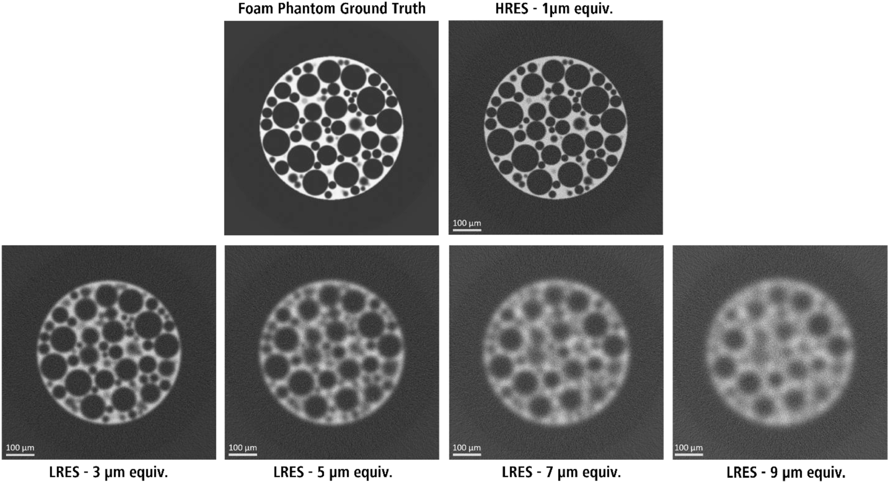
The foam phantom images used to train the DeepNet models in this study. The low-resolution images (LRES – 3, 5, 7, and 9 µm) were paired with the high-resolution (HRES – 1 µm) image for training.
For this study, two realizations of the foam phantom were considered. The 512 × 512 × 512 voxel phantoms were forward projected modeling cone-beam micro-CT acquisition geometry generating 512 projections over 360° angular range. The forward-projected images were blurred with a 2D Gaussian filter and introduced a fixed value of Poisson noise. These datasets were then back-projected using the FDK algorithm to generate reconstructed images. Varying levels of image quality degradation were considered by increasing the strength of the Gaussian filter to simulate increasing losses in spatial resolutions of the final images. In this study, these simulated datasets are referred to by their representative spatial resolutions-1, 3, 5, 7, and 9 µm, where the number represents the standard deviation of the Gaussian blurring function (Figure 1).
Both realizations of the foam phantom have a randomized structure, with the same number of total pores within the bulk volume (∼1,400) and a similar distribution of the pore sizes. However, the structural difference arises mainly from the spatial positioning and clustering of the pores within the foam bulk. The ground truth images for both realizations were generated by increasing the number of image projections to a high quantity, close to 6,000, for the reconstruction. This allowed for noiseless and realistic representation of the phantoms, serving as ground truth for comparison.
2.3 Real-world applications
The performance of DeepNet was also evaluated with case studies involving real-world datasets. A dried western sycamore seed with multiscale features was selected as a candidate sample for a similar analysis to the foam. The Seed exhibits internal features such as pores, tubules, and shell-like layers. This sample has a bimodal pore distribution, with the smaller pores discernable only when imaging at higher spatial resolutions, as such, it serves as an ideal sample for assessing the feature recovery performance. An integrated circuit was also studied to highlight the feature recoverability and data upscaling.
The Seed and Chip samples were scanned in a cone-beam imaging geometry with a Zeiss Xradia Versa 630 (Carl Zeiss X-ray Microscopy, Dublin, CA) equipped with a 30–160 kV X-ray source. The images were captured with a CCD sensor system with interchangeable scintillator-based objectives for optical magnification. The geometrical magnification from the diverging source X-rays, coupled with the optical magnification of the detector system, allows scanning images at voxel sizes as low as 0.3 µm. Taking advantage of this multi-resolution imaging capability, data acquisitions were carried out at different voxel sizes to obtain different training pairs for DeepScout, while ensuring the HRES dataset was aligned within the selected LFOV image. The acquisition parameters were optimized to capture the relevant features for evaluation and are listed in Table 1.
Acquisition parameters of the samples used in this study.
| Sample | Voxel | Objective | Det. pixel | Field | Source | Source to | Sample to | # of | Exposure per | |
|---|---|---|---|---|---|---|---|---|---|---|
| size | bin | of view | energy | sample dist. | detector dist. | projections | projection | |||
| Seed | LRES | 9 µm | 0.4X | 2 | 18.4 × 18.4 mm | 50 kV | 39 mm | 110 mm | 2,401 | 5 s |
| MRES | 3 µm | 4X | 2 | 3.1 × 3.1 mm | 50 kV | 19 mm | 23 mm | 3,001 | 1.5 s | |
| HRES | 1 µm | 4X | 1 | 2.1 × 2.1 mm | 50 kV | 19 mm | 40 mm | 3,501 | 9 s | |
| Chip | LRES | 6.75 µm | 0.4X | 1 | 13.8 × 13.8 mm | 110 kV | 44 mm | 180 mm | 2,401 | 5 s |
| MRES | 2.25 µm | 4X | 2 | 2.3 × 2.3 mm | 110 kV | 44 mm | 88 mm | 2,001 | 9 s | |
| HRES | 0.75 µm | 4X | 1 | 1.5 × 1.5 mm | 110 kV | 44 mm | 154 mm | 2,401 | 25 s | |
-
Note: MRES is medium resolution.
2.4 Training super-resolution models
The DeepNet training for all the low-resolution simulated foam phantom volumes (3–1, 5–1, 7–1, and 9–1 µm) was performed by pairing each with the target HRES 1 µm image. To highlight the versatility of DeepNet, two randomized realizations of the foam phantom were utilized. The first set of images was used to train the neural network models by pairing the HRES image (1 µm) with different LRES counterparts (3, 5, 7, and 9 µm). The second set of foam images, referred to as ‘alternate’ images in this study, are not seen by the model during the training phase. These alternate datasets are similar to the training counterparts but have a different spatial distribution of pores within the volume. The trained models were then used on both the training and the alternate realizations to infer the respective LRES images (flowcharts within [30]). The HRES-MRES and MRES-LRES pairs with a resolution ratio of 3:1 were selected for the Seed and Chip datasets, where MRES is the medium resolution image between high and low resolution images.
The seed and the integrated circuit training pairs were spatially registered to match the corresponding subvolume of the LFOV low-resolution image with the target high resolution image volume. The spatial coordinates for each image are derived from the sample stage motor positions, which aid in coarse registration. The 3D image registration is then fine-tuned to ensure the perfect superimposition of both images using a custom FFT-based registration algorithm based on prior patents [40], [41], expanded to 3D use micro-CT use case. This is an automated integral part of the DeepScout workflow, requiring only the training images as input for the registration, after which DeepNet is utilized to initiate the training of the super-resolution model.
2.5 Image processing, segmentation and evaluation
Image quality metrics such as the means square error (MSE), structural similarity index (SSIM), and peak signal-to-noise ratio (PSNR) for the results in comparison to the ground truth images, were calculated using Dragonfly (Object Research Systems, Montréal, Canada). The image processing and segmentation were done with Avizo (Thermo-Fisher Scientific, Waltham, MA). The results for DeepNet and SRCNN were analyzed without any further denoising step. Some of the high resolution or low resolution images were additionally denoised with deep-learning based edge preserving image denoising method (commercially available from Carl Zeiss X-ray Microscopy as ZEISS DeepRecon Pro) for comparison [42].
An image-agnostic route was critical to evaluate the ease of feature recovery without manual intervention to highlight the usability of the images in realistic use-case scenarios for data quantification. Therefore, an automated image analysis workflow was used to evaluate the feature recovery – (a) automated thresholding to identify the pore space and create a binary image, (b) fill small holes using a closing operation, (c) separate merged objects, and (d) followed by object analysis for quantitative measures. For the quantitative analysis, the segmented pores connected to the top and bottom slices were removed using an edge-kill script to avoid considering dissected pores at the ends of the Foam images, to ensure morphological analysis was not affected (see Supplementary Material; Figures S1, S2 and Section S1). A non-local means filter (NLM) was used for the Richardson-Lucy images only before the automated thresholding step to reduce noise and prevent over-segmentation.
2.5.1 Gaussian fit analysis
A Gaussian fit method was employed to provide a quantitative measure of spatial resolution loss when using different imaging setups. The higher-resolution image was repeatedly convolved with a 3D Gaussian kernel until the best least squares fit was identified between the convolved image and the lower-resolution volume. The FWHM of the Gaussian kernel that provided the best fit would then serve as the measure of spatial resolution difference. This method is insensitive to hallucinations and evaluates the spatial resolution of the images.
2.5.2 Multiscale-SSIM
Multiscale-SSIM (3D) index was used to generate quality maps for the processed images with respect to the ground truth phantoms as a reference, with an in-built MATLAB (Ver. R2024a) function (multissim3) [43]. The multiscale-SSIM index for the quality maps combines the SSIM index of several image versions at different scales (i.e., downscaled resolutions) to output a local value for each voxel within the 3D volume. Similar to SSIM, a value closer to 1 indicates a good match with the ground truth, while a value closer to 0 indicates poor quality. The clustered voxels with lower values, therefore, correspond to regions with a higher probability of hallucinatory features to be present.
3 Results and discussion
3.1 Foam phantom
A visual comparison of DeepNet results on the Foam realizations showed excellent noise-free and detailed images when the trained models were applied both on the training datasets and a separate realization of the same phantom dataset that was not seen by the training process (Figure 2). Notably, this highlights the robustness of the algorithm, demonstrating its capability to effectively process images beyond its immediate training domain, if the features in the targeted images are similar and comparable to training datasets.
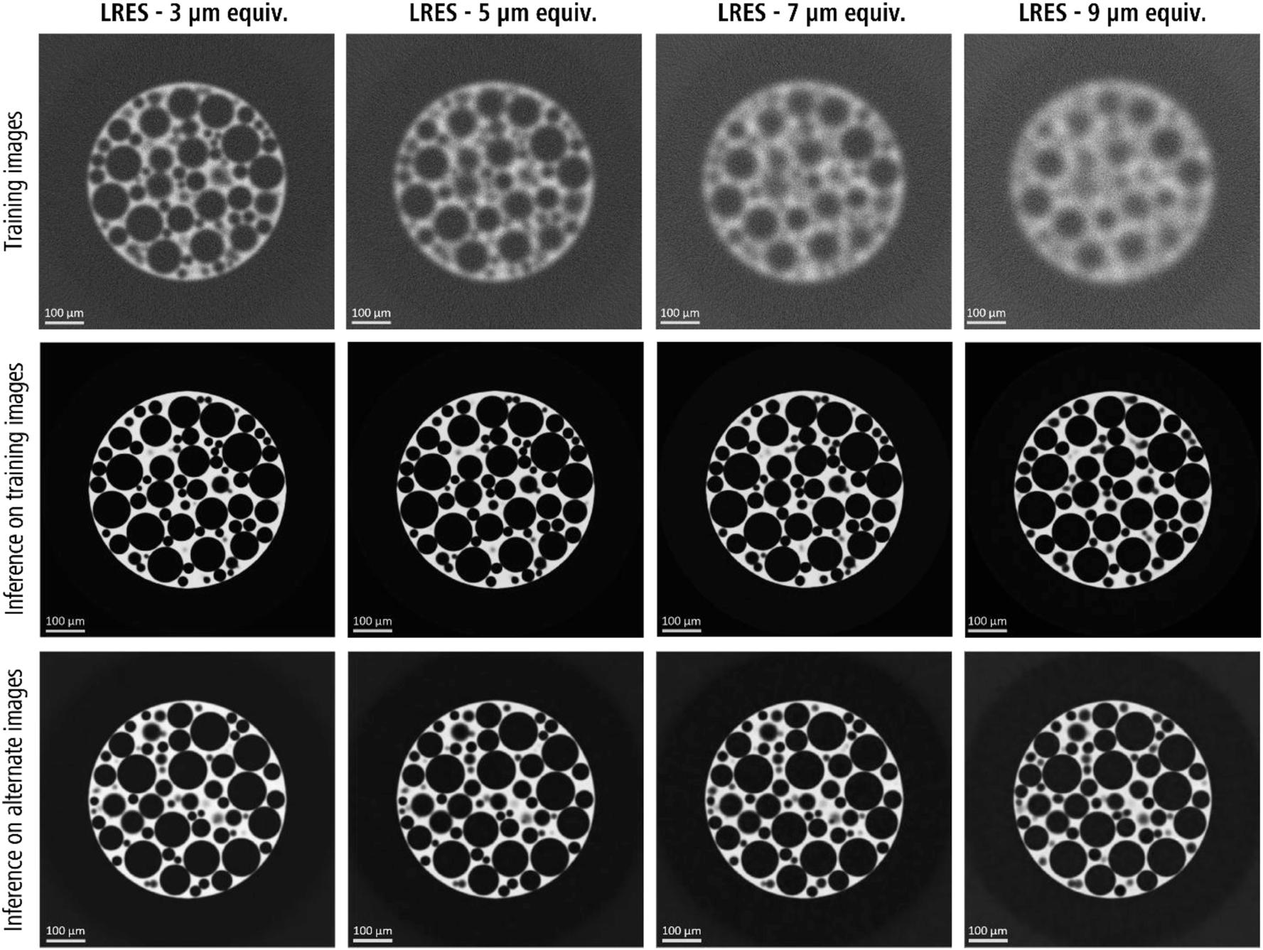
A comparison of the DeepNet inference results on both the training and an alternate realization of the foam phantom. Note: Refer to Figure 8 for the ground truth of alternate dataset.
3.1.1 Image quality
The feature recovery performance of Richardson-Lucy, SRCNN, and DeepNet algorithms was evaluated quantitatively by comparing them with the generated ground-truth foam phantom image. The Foam datasets shown in Figure 1 were used to train both DeepNet and the SRCNN models, which were then applied to the alternate realization of the Foam. For consistency, the quantitative metrics were compared between the results from the alternate realization of the Foam for all three algorithms.
Figure 3 presents a quantitative assessment of the image quality using three widely adopted metrics: mean square error (MSE), peak signal-to-noise ratio (PSNR), and structural similarity index measure (SSIM). Along with unique insights into image quality, these metrics also provide an objective comparison of the images with respect to the ground truth, avoiding human subjectivity. However, it should be noted that they have their limitations. MSE and PSNR are insensitive to structural changes and, therefore, lack correlation with perceived image quality [44]. Lower MSE values and higher PSNR signify a closer representation of the ground truth in terms of pixel intensity distribution and signal strength to the noise, which might not be a complete representation of the actual image quality [45]. The SSIM instead aids in assessing the preservation of structural details, with higher image quality corresponding to values closer to 1.
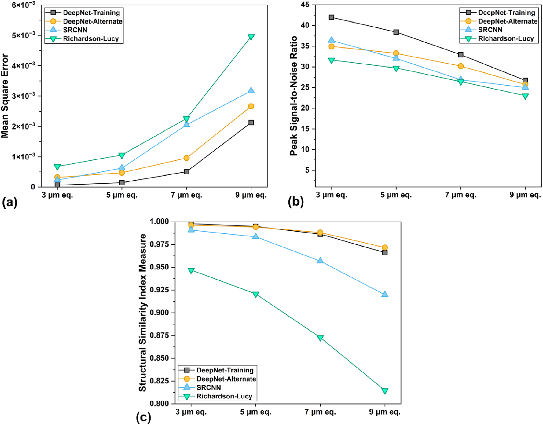
Image quality metrics (a) mean square error (MSE, lower is better), (b) peak signal-to-noise ratio (PSNR, higher is better), and (c) structural similarity index measure (SSIM, closer to 1 is better), of all the images analyzed in this study.
With the deterioration in spatial resolution, the image quality metrics worsened for all methods. This is expected because of the increasing resolution ratio between the ground truth and the input images. DeepNet consistently outperformed the other two methods across all metrics and resolutions. The lower MSE, higher SSIM, and high PSNR values suggest its effectiveness at pixel-level accuracy and overall structural preservation. The SRCNN followed slightly behind but with a steeper drop in image quality at lower resolutions, especially lacking in feature preservation. While SRCNN and DeepNet inference on the alternate foam realization for 3 µm, show comparable MSE and PSNR performance, the following results diverge as the shallow network of SRCNN cannot compensate for larger resolution losses. Furthermore, the deeper network architecture of DeepNet ensured a higher SSIM and, therefore, a lower probability of hallucinatory artifacts. Richardson-Lucy demonstrates reasonably good performance as a classical deconvolution method, at least according to these quantified metrics. The low SSIM (∼0.94), even for the 3 µm image, suggests that it fails to recover certain structural features, which is only exacerbated with increasing resolution ratios. In the end, both CNN algorithms show better recovery than RL, from the learned correlations between the LRES and HRES pairs during the training step.
A qualitative comparison of the central XY slice of the results for the alternate Foam realization with each algorithm, along with the noisy input images with varying degrees of image degradation, is shown in Figure 4. Visual assessment of the images provided additional information for evaluating these algorithms. The classical RL deconvolution method severely underperformed, with blurry images, lowered brightness, and reduced edge contrast. The smaller features become unrecoverable at lower resolutions (i.e., 7 and 9 µm), while the larger features were reduced in size due to edge blurring. Clusters of small pores were either lost or incorrectly recovered as fused irregular, larger-sized pores. Additionally, speckling artifacts were apparent in the bright phase despite good noise reduction in the darker regions.
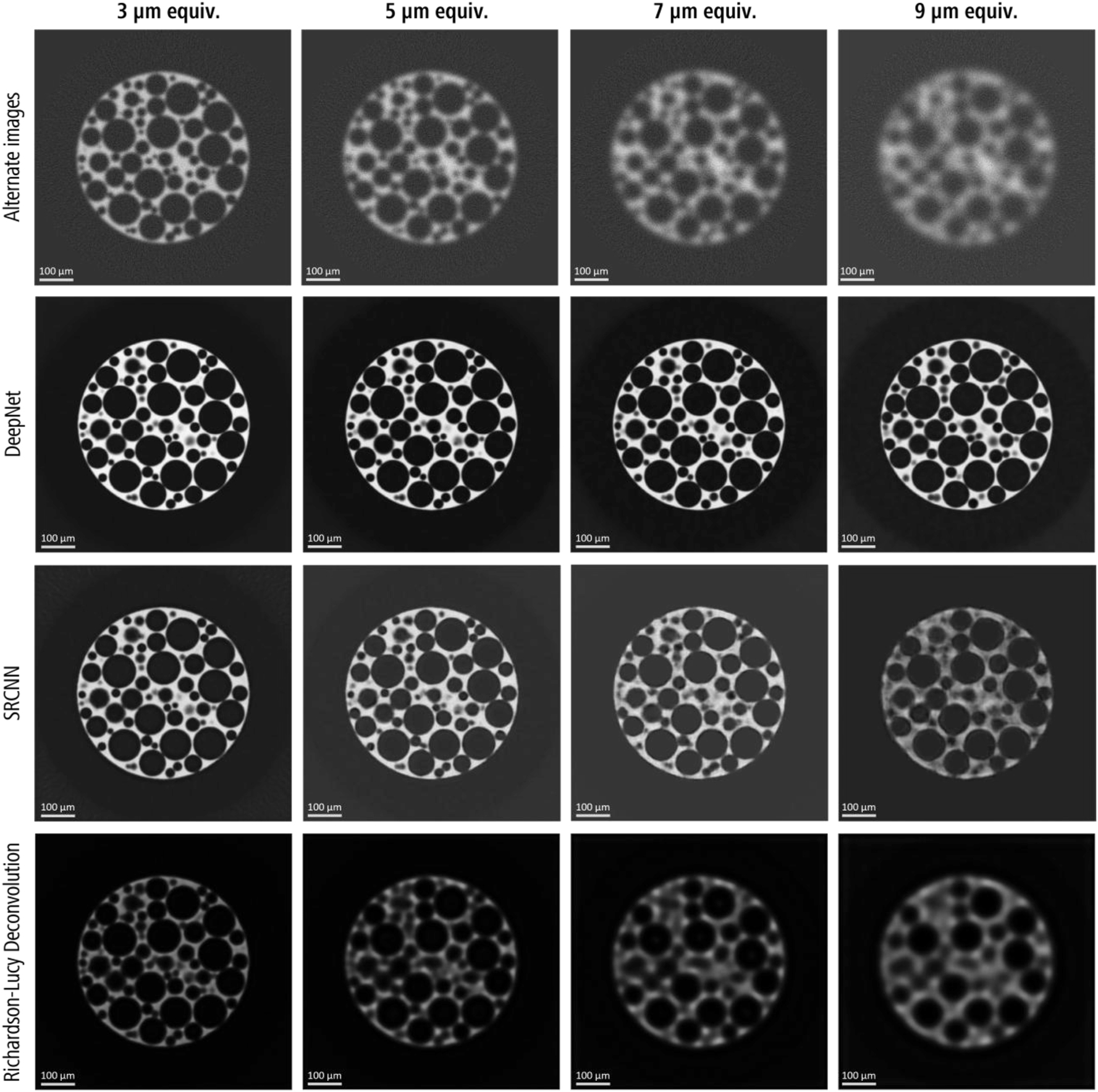
A qualitative comparison (slice # 256/512) of the resolution recovery performance with DeepNet, SRCNN and Richarson-Lucy deconvolution models with the degrading image quality of the alternate foam realization. The input images are shown in the top row. Note: Refer to Figure 8 for the ground truth of alternate dataset.
Although the image quality metrics were suboptimal for SRCNN (Figure 3), visual inspection reveals a good improvement over RL deconvolution, especially for 3 and 5 µm images. On closer examination, these images had certain textural artifacts in both dark and bright phases of Foam, confirming these small differences at a pixel level largely impacted the image quality metrics. Furthermore, SRCNN was ineffective in preserving smaller pores at lower resolutions (i.e., 7 and 9 µm), while the larger pores were mostly preserved. Similar to RL, clusters of small pores were recovered as merged irregular pores. The 9 µm image exhibited a severe recovery loss, with distinct textural artifacts near the edges of larger pores and the bulk phases. These artifacts are most likely due to the image hallucinations during the model inference step, exacerbated by larger resolution ratios.
DeepNet showed excellent recovery across all four resolution scales along with edge preservation. Similar to SRCNN, it inherently denoises the images during training since the training pair contains two independent noise realizations but results in very few textural artifacts, even for the recovered 9 µm image. However, some visual discrepancies were observed for the 9–1 µm images, particularly for the smaller pore sizes. These are most likely due to the large resolution gap between LRES-HRES training pairs, potentially resulting in image hallucinations during inference.
3.1.2 Quantitative feature evaluation
To quantitatively assess the performance of the algorithms in recovering the structural details, the foam images were analyzed as porous materials, enabling the comparison of porosity and pore size distributions with the ground truth. The same automated image processing workflow, initially optimized for the ground truth images, was applied to all the results. It allowed a comparison of the results from each recovered image to the ground truth, which serves as baseline. The quality of the results could have a minor effect on the segmentation and the separation of pores that are closer to each other, due to noise, lack of contrast or blurred edges.
The pore recovery performance, presented as the percentage of pores identified relative to ground truth (1,380 pores for both realizations) with automated segmentation, is shown in Figure 5. DeepNet recovered over 95 % of the pores detected for low resolutions (3, 5, and 7 µm) when applied to both the training and the alternate datasets (Figure 5). Even with a high-resolution ratio at 9 µm, it recovered over 85 % of the pores, demonstrating strong recoverability performance. In contrast, the SRCNN model performed well for the 3 and 5 µm images but showed a linear decline in recovery for reducing resolutions, to only 60 % at 9 µm. Richardson-Lucy method exhibited the poorest performance with suboptimal recovery even for the highest resolution (3 µm) image, followed by a sharp decrease at lower resolutions.
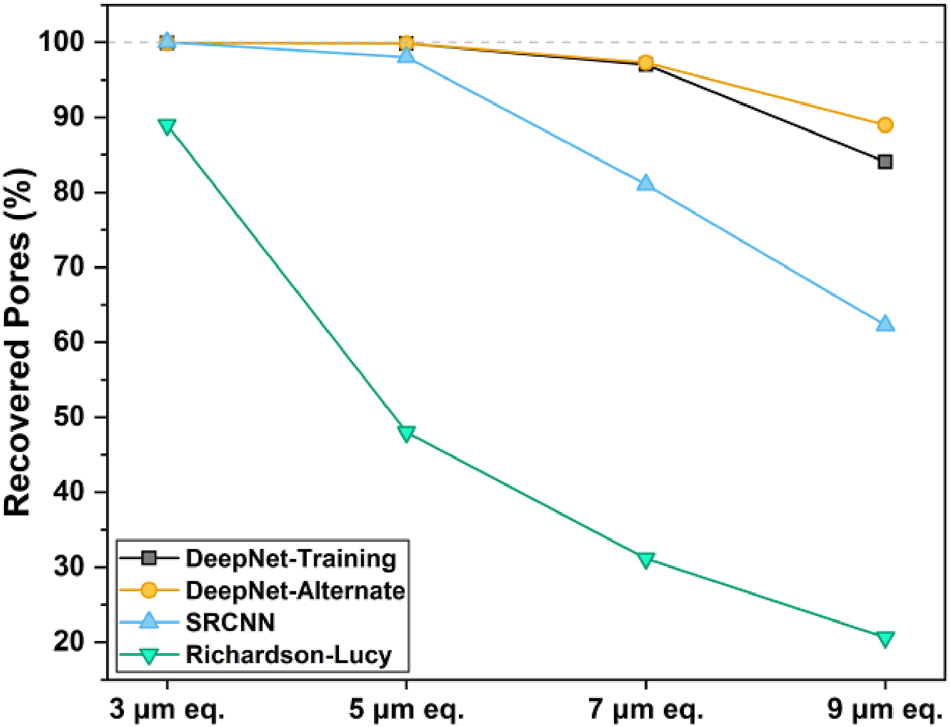
The percent pore recovery performance of the algorithms evaluated in this study, with respect to the ground truth. The baseline count for the ground truth was calculated to be 1,380 pores, which was used as a reference.
While pore recovery performance shows the effect of the recovered image quality on quantification, further analysis was carried out to study recovery of pores based on their total volume, sizes and shape. Figure 6 shows a quantitative comparison of porosity and pore size distributions between the processed images and the ground truth. The porosities, calculated as the ratio of pore volume to the foam’s bulk volume mask, are indicated within the label boxes. The pore size distributions are plotted as histograms with a 5 µm bin width, where the spherical equivalent diameter of the volume of each segmented pore represents the sizes.
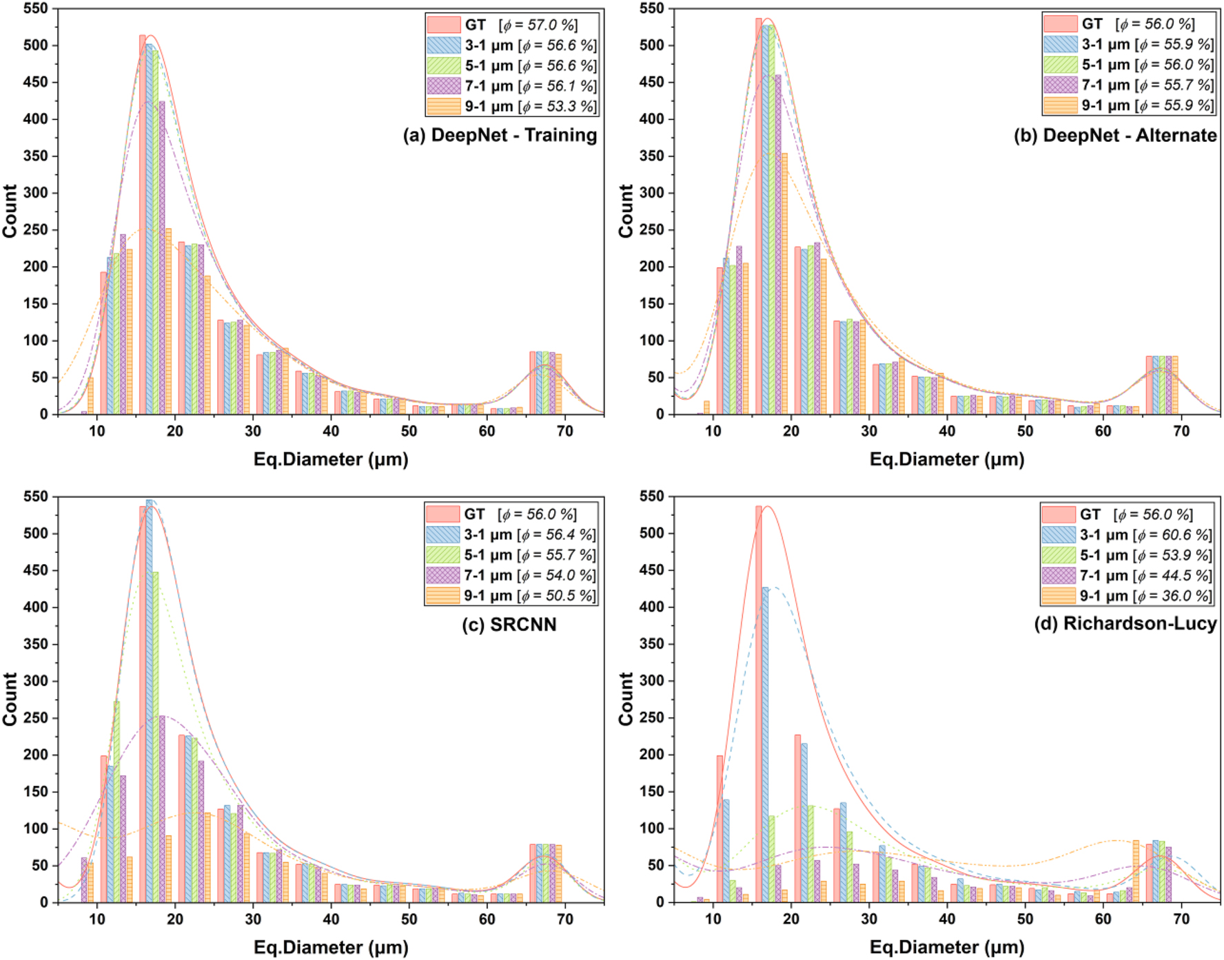
Quantitative comparison of the porosity and the pore size distributions of the foam datasets with the ground truth as a reference. The porosities (ϕ) are highlighted in the label boxes. Note: Panel (a) shows results of DeepNet model on the training data, while (b), (c) and (d) show the results of DeepNet, SRCNN, RL for the alternate foam realization.
Although the total pore recovery with the RL algorithm was below 90 % for the 3 µm image, the porosity estimate was higher than that of the ground truth (Figure 6d). This was primarily due to the insufficient edge contrast affecting the segmentation of large pores (diameters greater than 25 µm), resulting in larger diameters than those from the ground truth. In contrast, the lower pore count was mainly due to the loss of small pores with diameters below 20 µm. The porosities and the recovered pores declined sharply, with a decrease in the spatial resolution of the input images.
The SRCNN results for the 3 µm image exhibited an excellent match with the ground truth both for pore recovery and size distributions. The porosity estimates for all resolutions were within 10 % of the actual value, mainly due to the recovery of large pores (Figure 6c). However, lower resolutions negatively affected the smaller pores (diameters below 25 µm).
DeepNet shows superior pore recovery across multiple resolutions (Figure 6a and b), with recovered porosities for both Foam realizations within 6 % of the ground truth baseline. The pore size distributions indicate that the trained models accurately recover the medium to large-sized pores (i.e., between 25 and 70 µm), while the losses were primarily from the smaller pores. Additionally, the results from the inference images indicate that pore recovery of smaller pores was better than that on the training images. This is most likely the reason for the slightly higher percent pore recovery with the application of trained models on the alternate Foam realization shown in Figure 5. Notably, the remarkable recovery of pores larger than 60 µm for all images highlights the ability of DeepNet to recover large features accurately, provided the loss in spatial resolution does not overshadow the feature sizes.
While the pore size distributions show how the models recover the segmented pores, they fail to identify how accurately the features are recovered. This is especially important for lower spatial resolution images, where some of the smaller pores have sizes comparable to the standard deviation of the applied Gaussian blurring function. For low-resolution data, clusters of tiny pores could be inferred as voids with irregular shapes, which cannot be identified with equivalent diameters. To address this, the sphericity parameter was analyzed, with values ranging between 0 and 1, which defines how closely the shape of a feature resembles a perfect sphere (with 1 representing a perfect sphere):
where V and A are the volume and boundary surface area of the segmented pore.
The average sphericity of the pores for the ground truth Foam images was found to be 0.990. While smaller pores have a pixelated irregular surface area, resulting in values slightly lower than 1, the majority of the segmented pores were within an acceptable range of 0.975 and 1 (refer to Figure 7). Due to stochasticity in the pore shapes and sizes, the surface area estimates for the segmented pores, although accurate, might not be precise. In our study, this resulted in sphericity values greater than 1 (in the third decimal), which were treated as outliers and rounded to 1.

The box plots of the sphericity parameter as a metric to evaluate the accuracy of the recovered features compared to the ground truth. The horizontal line within the box represents the mean (also shown with a numeric label), and the whiskers represent the standard deviation. The data points are shown as an overlay for visual reference. Note: Panel (a) shows results of DeepNet model on the training data, while (b), (c) and (d) show the results of DeepNet, SRCNN, RL for the alternate foam realization.
The sphericities of the recovered pores with different models are presented as box plots in Figure 7. The average sphericities with RL deviated considerably from the ground truth, even for the 3 µm image (Figure 7d). For lower resolutions, the averages decreased further before increasing again. This is primarily due to the inability of the RL method to recover most pores (as can be observed visually in Figure 4), while the increased sphericity for the 7 and 9 µm images was due to the large, rounded pores being recovered, skewing the averages.
The SRCNN models fared better for the 3 and 5 µm images, with the averages closer to the ground truth. However, lowered average sphericities and larger standard deviations were observed for the 7 and 9 µm images. Although SRCNN recovered up to 60 percent of the total pores, the lowered sphericity indicates that most were poorly defined. This is most likely due to the hallucinatory effects that are exacerbated by noise and low spatial resolution.
The DeepNet models exhibit a remarkable recovery in pore shapes for resolution ratios up to 7:1. Notably, the average sphericities for all images were within 5 % of the ground truth. Although most data points were clustered closer to 1, deviations as low as 0.75 were found for the 9 µm images. Further investigation revealed this was primarily due to hallucinatory artifacts propagating into the image during model inference.
3.1.3 Image artifacts and spatial resolution
The comparative study utilizing the simulated foam phantoms demonstrates that DeepNet excels in recovering both feature size and shape while inherently denoising the images. The selection of the HRES-LRES pairs and the magnitude of the resolution gap impacted the outcome. However, results support that excellent and reliable results are achievable, even with spatial resolution ratios of up to 7:1 between the input training images.
In real-world scenarios, image quality is influenced by a complex interplay of acquisition parameters such as source voltage (impacting contrast and beam hardening), number of projections and their exposure time (affecting the signal-to-noise), and voxel size (affecting the minimum resolvable feature size). Additional losses may arise from mechanical limitations of the instrument itself. Therefore, the loss in spatial resolution in the acquired image is due to a cumulative point spread function that is a combination of various effects that is challenging to address with conventional image restoration methods such as the Richardson-Lucy iterative deconvolution.
The complexity of this problem naturally pivots towards the reliance on advanced deep learning-based convolutional neural network approaches. While SRCNN shows excellent feature recovery with small resolution differences between the HRES and LRES images, DeepNet leverages its deeper network architecture and a much larger number of trained parameters. It recovers image sharpness over wider resolution differences and retains the features within the phantom. This result aligns well with the findings of the previous work [46], [47].
Multiscale-SSIM (MS-SSIM) quality maps were generated for the 3 and 9 µm images of the alternate foam realization (Figure 8) to provide a spatially resolved assessment of localized image fidelity relative to ground truth. In these maps, darker regions correspond to higher MS-SSIM values (close to 1), indicating strong structural similarity, while the brighter areas signify lower values, highlighting regions of potential structural dissimilarity and possible hallucination artifacts.

A comparison of the multiscale-SSIM quality maps of the 3 and 9 µm results for the alternate foam realization. The brighter hotspots represent the pixels with low SSIM values, highlighting the uncertainty of the recovered structural features. Note: The SSIM scale for the colormap varies for each quality map.
The DeepNet reconstructions demonstrated high fidelity, as evidenced by the predominantly dark MS-SSIM maps for both 3 µm and 9 µm resolutions. In the 3 µm image, subtle brighter regions are primarily observed at pore boundaries, likely attributed to minor discrepancies in edge sharpness. However, in the 9 µm image, more pronounced bright hotspots emerge, particularly in areas with smaller pores. These localized reductions in MS-SSIM suggest either the presence of spurious pores (hallucinations) or the absence of actual pores in the reconstruction, leading to structural mismatches with the ground truth.
In contrast, the RL and SRCNN reconstructions exhibit more extensive regions of brightness in their MS-SSIM maps, especially at 9 µm resolution. This indicates widespread structural dissimilarity and a higher prevalence of artifacts or distortions. Among the CNN algorithms, the SRCNN images show regions of extreme brightness, suggesting a greater probability of generating hallucinatory features. Textural inconsistencies (shown in Figure 4) present for both SRCNN and RL further support this observation.
Figure 9 shows the results for the Gaussian fit analysis for the alternate Foam images, highlighting the mean square error (MSE) when compared to the ground truth image convolved with increasing Gaussian blur kernel size from 0 to 10. The calculated MSE quantifies the discrepancy between the blurred ground truth image and the images processed using different algorithms. A higher error at lower kernel sizes arises from the high-frequency features or hallucinations present in the image compared to the blurred ground truth. At higher kernel sizes, the image becomes dominated by over-blurred features, resulting in a significantly larger MSE. Generally, the Gaussian kernel size corresponding to the lowest error for each curve can be considered the effective spatial resolution of the recovered images.
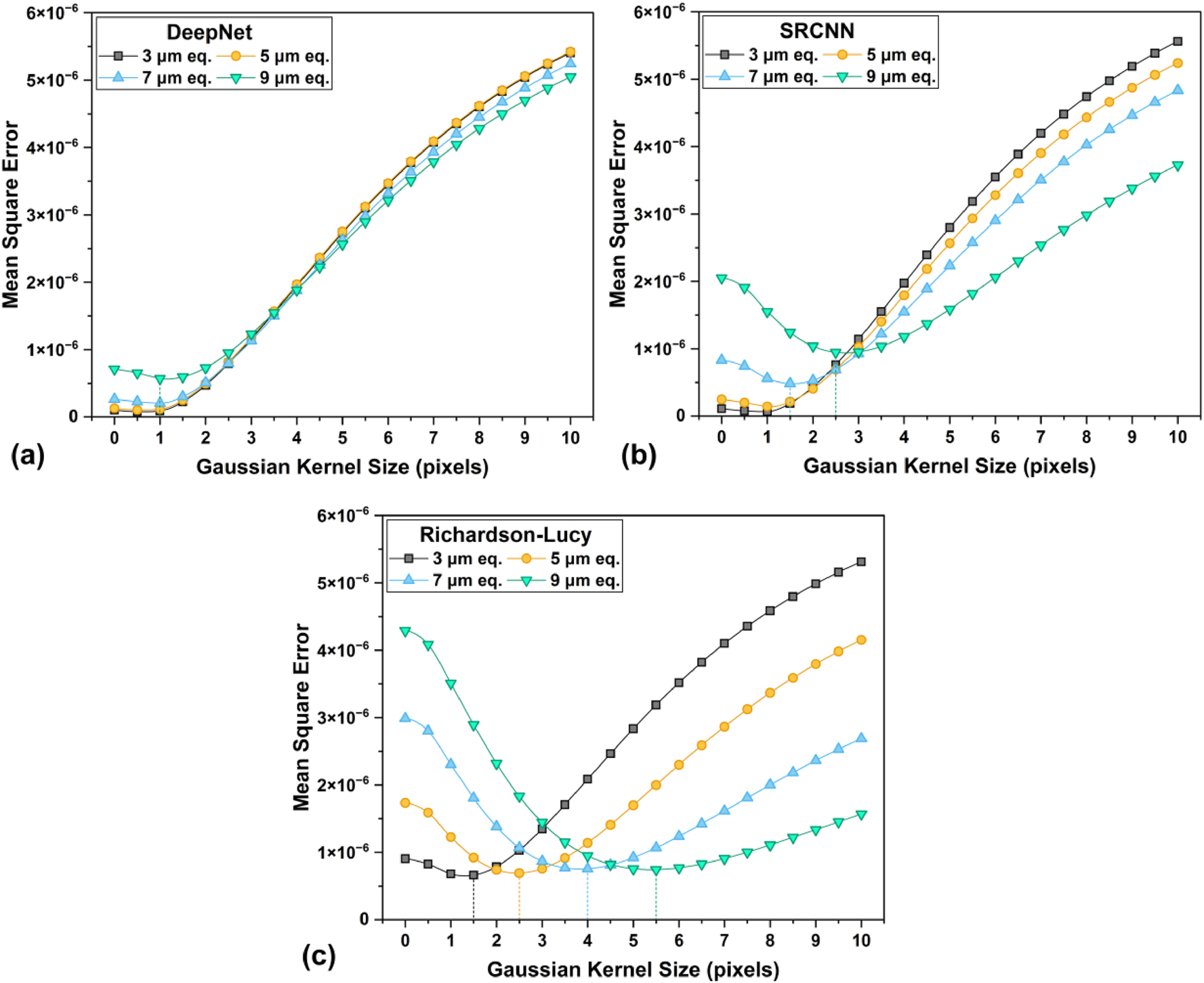
A comparison of the effective spatial resolution of results from each algorithm on the alternate foam realization, with the Gaussian fit analysis. The lowest point of error for each curve (highlighted with droplines) corresponds to the Gaussian kernel size of the convolved ground truth image, with the best match.
These findings suggest that CNN based algorithms show large improvements in the effective spatial resolution compared to classical methods. While RL shows a reasonably good outcome for the 3 µm image, it fails for images with more severe image quality degradation. Among the CNN models, DeepNet outperforms significantly, with the effective spatial resolution of its images closely matching the ground truth. The SRCNN models perform well at lower degradation levels but exhibit a faster decline with increasing image quality loss. With deeper neural network architectures like DeepNet, it is possible to recover image resolution that closely matches the ground truth, even with severe degradation.
The multi-faceted image analysis conducted on the simulated foam phantoms comprehensively evaluated the performance of each algorithm from different perspectives. While DeepNet demonstrates remarkable feature recovery capabilities, as evidenced by the quantitative analysis, the MS-SSIM quality maps reveal the potential for hallucinations, particularly at higher resolution ratios, which can compromise data reliability. However, within the recommended resolution limits (up to 7:1, depending on the sample’s fine features), DeepNet exhibits exceptional performance. It is crucial to acknowledge that imaging artifacts, such as photon starvation or phase artifacts, can negatively impact the training process. These artifacts may be misinterpreted as genuine features during training, leading to erroneous propagation into processed images during inference.
3.2 Applications in real-world scenarios
Some recent publications focusing on additive manufacturing [48], materials science [49], [50], batteries [51], electronics [1], and packaging failure analysis [52], describe DeepNet’s practical applications for high-resolution LFOV and feature recovery as part of the DeepScout workflow. In a specific use case, Cognigni et al. leveraged the utility of DeepNet, for a resolution ratio as high as 6:1 to investigate fungal distribution on polyethylene terephthalate (PET) fragments [49].
Figure 10 shows a realistic use case scenario for DeepNet for resolution upscaling with LRES-MRES (6.75–2.25 µm) and MRES-HRES (2.25–0.75 µm) training pairs of an integrated circuit. The FDK reconstructions (Figure 10 top row) show magnified (for LRES and MRES) subvolume slices of the micro bumps generally found in these semiconductor devices. Although the LRES image has LFOV, the image is unusable for defect analysis and metrology due to the lack of spatial resolution. The defects in the same location can be identified with the MRES image, albeit with a smaller FOV. When trained with DeepNet, the model successfully recovered the image quality over the entire LFOV scan, enabling easier defect recognition and failure analysis. With the higher resolution pair (MRES-HRES), increased sharpness and details of the defects were recovered, along with finer details closely matching the 0.75 µm image.
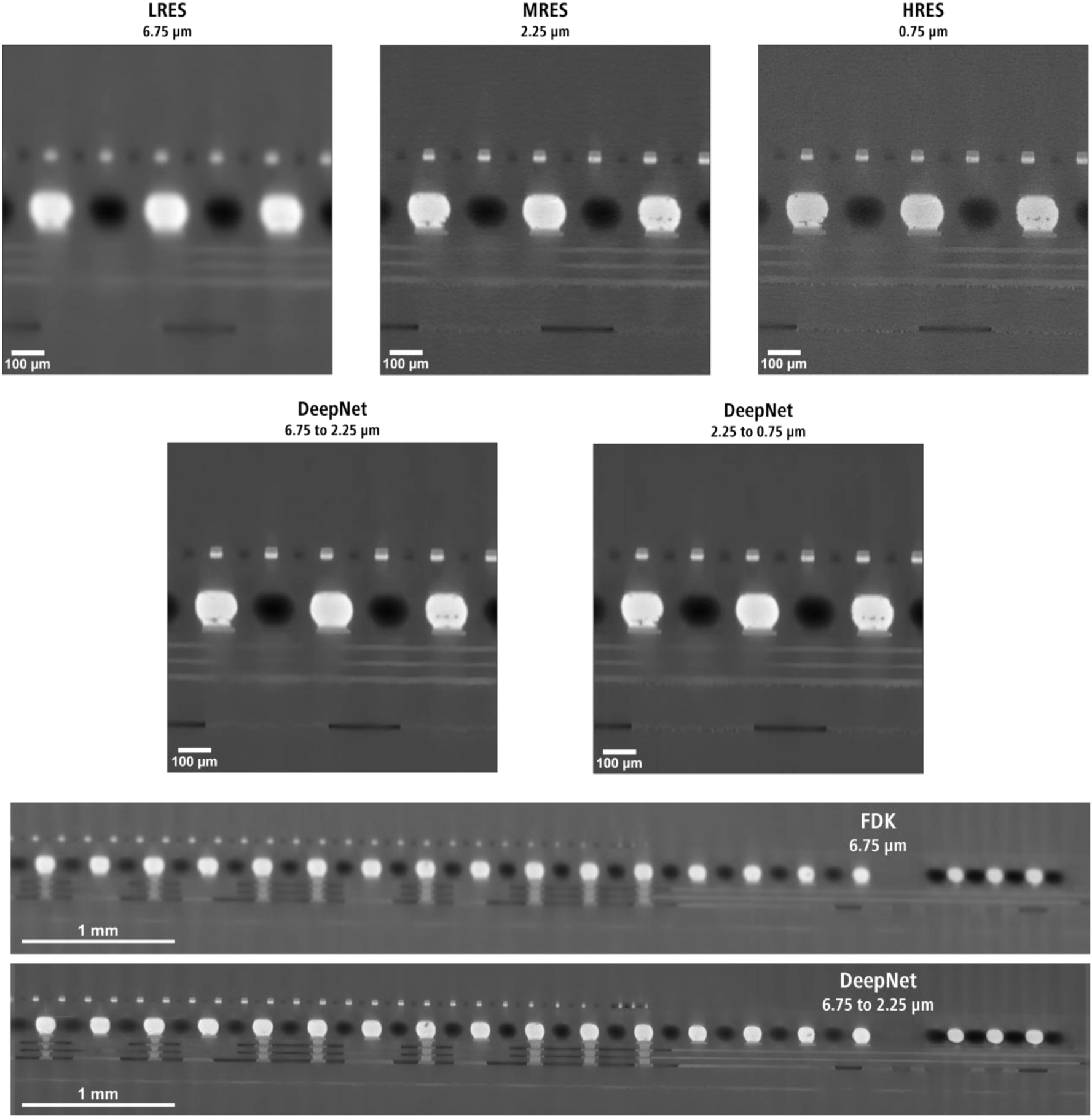
A comparison between the FDK reconstruction images and the DeepNet inference results for the integrated circuit acquired at three different voxel sizes. The large field of view (wide aspect ratio) subvolume comparison between the FDK reconstruction and DeepNet result is shown at the bottom.
Although this sample benefits more from a higher resolution ratio for recovering even finer details with the LRES-HRES pair (i.e., 6.75–0.75 µm), it results in an extremely large upsampled image size after the inference. For example, with the resolution upscaling from 6.75 to 2.25 µm is performed, the image file size increases by 27 times, with exponentially higher values for increasing resolution ratios. To overcome this, the model can instead be applied to a smaller region of interest to ensure the imaging data is still practical to use and store on a regular workstation.
A similar application on the western sycamore seed improved the resolution of a 9 µm LFOV scan with a 3 µm HRES pair (Figure 11) with DeepNet training. The learned model improved features such as the pores, tubules, and porous outer shell, greatly enhancing the finer details. These use cases show the versatility of DeepScout workflow, where small subvolumes can be upscaled rather than the entire LFOV for targeted investigations. Figure 11 shows a magnified slice-to-slice comparison between results for three scans acquired at 9, 3, and 1 µm voxel size, reconstructed with classical FDK reconstruction in the bottom row. Although these reconstructed images are noisy and have varying contrasts (due to the differing CT acquisition parameters), the large features, such as pores, can be correlated with a manual inspection.
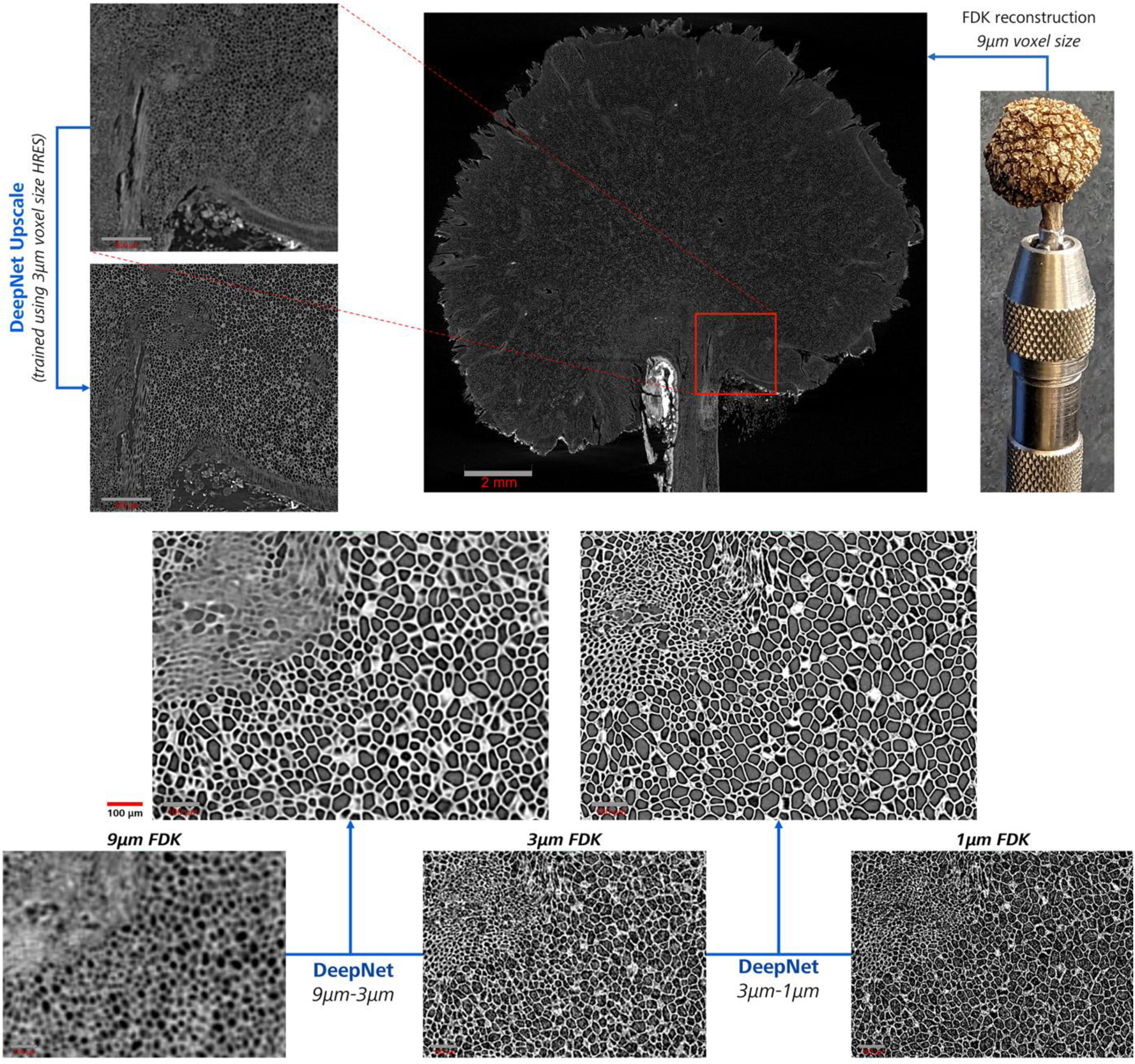
The inset shows (red square) the medium resolution subvolume (3 µm) within the large field of view (9 µm) micro-CT scan of the dried western sycamore seed. A direct side-by-side comparison of the image quality improvement with DeepNet with respect to the standard FDK reconstructions of the seed with intricate internal features is shown in the bottom grid at high magnification.
The LRES-LFOV 9 µm scan shows blurred features where only the large pores are distinguishable. A medium-resolution scan with 3 µm voxel size improves the image quality and detects additional smaller pores (top left of the slices) with higher spatial resolution. These smaller pores are resolved better at an even smaller voxel size (1 µm) due to higher spatial resolution. This is a common scenario for most microscopy use cases, where spatial resolution governs the detectability of the finer features, acting as a bottleneck.
The top row of the slice comparison shows the corresponding results from two DeepNet-trained models using the 9–3 µm and the 3–1 µm image pairs. Besides noise reduction, a large improvement in the sharpness of the images is evident from both models. Compared to the FDK reconstructions, the pores have better contrast and improved sharpness of the pore walls in the recovered images. The minor variations in the overall image contrast were mainly from the learned intensity correlations between the utilized input images. However, they have no direct effect on the usability of the images for segmentation.
Therefore, the reliance on mappable features between the input training images affects DeepNet training. This is also observed for the smaller pores in the result from the 9–3 µm model. DeepNet failed to create a reliable mapping during the training phase due to obscured finer details in the LRES (9 µm) image, as higher spatial resolutions were necessary to resolve the small pores.
A multiscale investigation was carried out on a small subvolume of the seed sample for quantitative comparison, leveraging its porous structure (Figure 12). The 1 µm scan was reconstructed with a deep learning denoising algorithm (DeepRecon Pro) to generate a sharp, noise-free image as a representative ground truth [42], [53]. Subsequently, 3 µm and 9 µm scans were also reconstructed with DeepRecon Pro to facilitate comparative evaluation at different resolutions. The slice-to-slice comparison of the analyzed subvolume (Figure 12) shows the differences in the denoised images (top row) and the DeepNet upscaled images (bottom row). Visual inspection demonstrates how DeepNet leverages both low- and high-resolution images to correlate and enhance features, which is evident in the subtle contrast differences and improved pore definition.
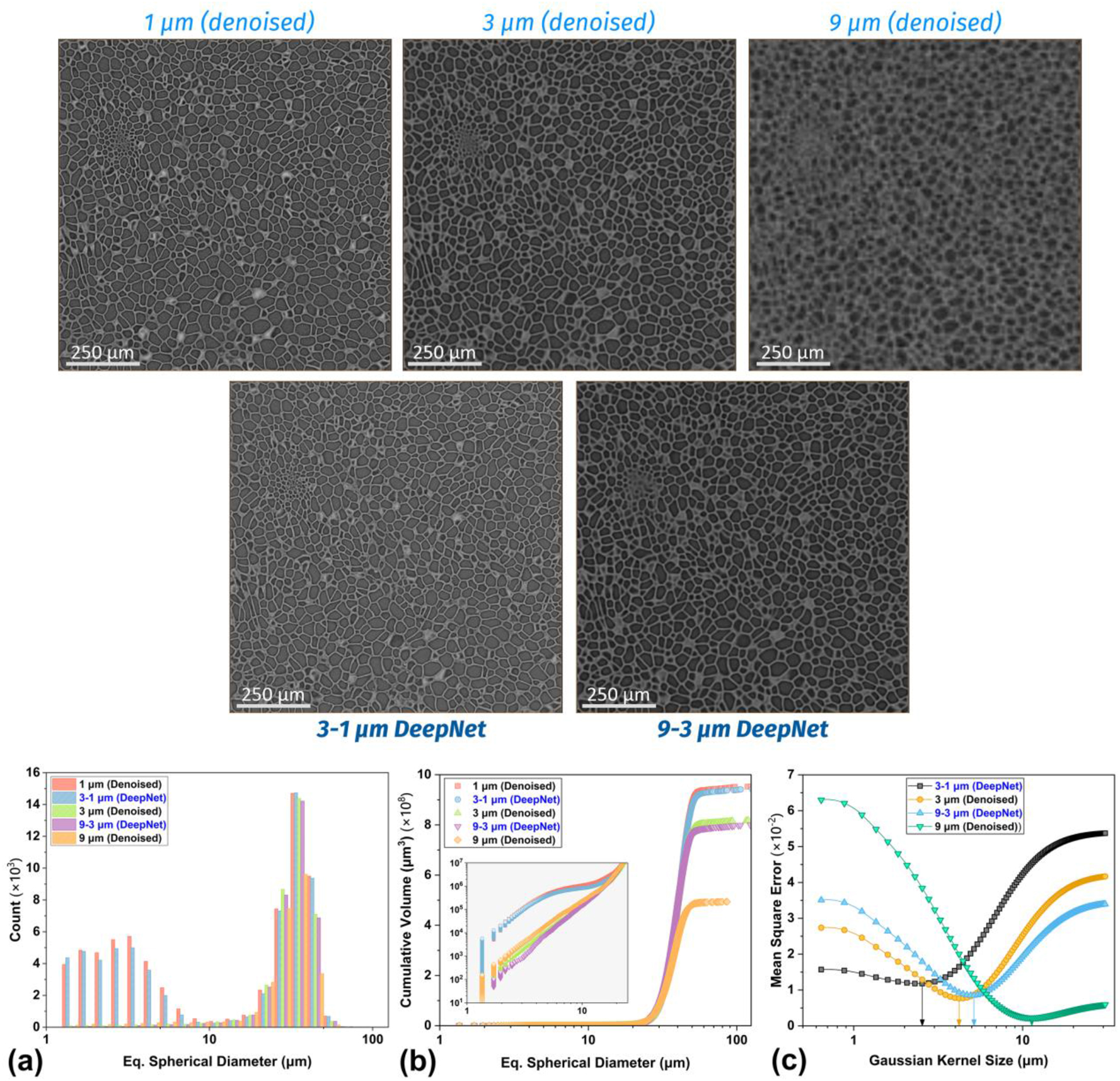
A comparison of the reconstructed slices of the seed datasets with DL-denoising (top row) and DeepNet training (bottom row). The (a) pore size distributions show that the smaller pores were recovered with the 3–1 um training due to better feature correlation but were absent for the 9–3 um training. A similar behavior can be found for the (b) total pore volume. The (c) Gaussian fit analysis shows the improvement in the effective spatial resolution because of DeepNet training.
For quantitative analysis, all images were resampled to the 1 µm voxel grid and segmented using the same automated workflow employed for the simulated foam phantom. The pore size distributions and cumulative pore volumes show a large improvement in the quantitative information, with each model closely matching its corresponding high-resolution target image. The trained 9–3 µm model improves the 9 µm image to match the pore size distributions and the pore volumes of the 3 µm image (Figure 12a). While smaller pores (<10 µm) remain undetectable, pore walls exhibiting strong correlation between the training images are significantly recovered, showcasing improved contrast and structural clarity. The 3–1 µm model further refines the reconstruction, recovering even the smaller pores to match the 1 µm ground truth closely.
The Gaussian fit analysis (Figure 12c), comparing the MSE between the ground truth and progressively blurred versions of the reconstructions, demonstrates a significant improvement in effective spatial resolution with the DeepNet models. This analysis, coupled with the pore quantification, highlights the reliability of DeepNet in recovering image quality without overinterpreting features when clear correlations are absent in the LRES image. By selectively enhancing features with high correlation between the training pairs, it minimizes the potential for hallucinations, ensuring the fidelity and usability of the recovered images.
4 Conclusions
A novel automatic convolutional neural network resolution recovery algorithm, DeepNet, designed to enhance the spatial resolution of large field-of-view micro-CT images, was evaluated. Its robustness lies in its ability to learn a spatially varying point spread function from pre-registered low and high-resolution image volumes. This facilitates resolution recovery across the entire LFOV while mitigating noise and sampling artifacts. The efficacy of DeepNet was rigorously evaluated with simulated phantom images that had increasing degrees of image degradation. The results were benchmarked against a classical iterative Richardson-Lucy deconvolution algorithm, and a deep-learning-based super-resolution CNN (SRCNN) algorithm.
The simulated phantom results demonstrated the superior performance of DeepNet in recovering features across a wide range of resolution gaps and in the presence of noise. It consistently performed better against the other two methods in terms of resolution and feature recovery, the accuracy of the recovered features, and lowered hallucinatory artifacts. Extending its application to real-world datasets with two different sample types further highlighted its practical utility in improving image quality and recovering complex features within the samples from low-resolution LFOV volumes based on feature correlation with a high-resolution subvolume image. Furthermore, its automated end-to-end imaging framework is highly versatile and user-friendly, only requiring the selection of image pairs for model training as the input. It is a promising approach for improving micro-CT workflows with potential applications in different use case scenarios and handling resolution ratios up to 7:1 between training pairs.
Acknowledgments
V.V.R.B. thanks Dr. Pankaj Sarin (Oklahoma State University) and Carl-Zeiss X-Ray Microscopy (Zeiss Innovation Center, California) for providing access to resources used in this study.
-
Research ethics: The conducted research is not related to either human or animals use.
-
Informed consent: Informed consent was obtained from all individuals included in this study.
-
Use of Large Language Models, AI and Machine Learning Tools: None declared. LLM, AI and ML tools were not used to develop or modify this manuscript.
-
Author contributions: V.V.R.B – Conceptualization, Investigation, Methodology, Formal Analysis, Validation, Visualization, Writing – original draft. M.X. – Investigation, Software, Writing – review & editing. M.A. – Conceptualization, Investigation, Software, Supervision, Writing – review & editing. A.A. – Conceptualization, Investigation, Software, Supervision, Writing – review & editing.
-
Conflict of interest: The authors declare that they have no known competing interests or personal relationships that could have appeared to influence the work reported in this manuscript. M.X., M.A., and A.A. are employees of Carl Zeiss X-ray Microscopy.
-
Research funding: None declared.
-
Data availability: Data is available upon request.
References
[1] H. Villarraga-Gómez, K. Crosby, M. Terada, and M. N. Rad, “Assessing electronics with advanced 3D X-ray imaging techniques, nanoscale tomography, and deep learning,” J. Fail. Anal. Prev., vol. 24, no. 5, pp. 2113–2128, 2024. https://doi.org/10.1007/s11668-024-01989-5.Search in Google Scholar
[2] H. H. Barrett and K. J. Myers, Foundations of Image Science, Hoboken, NJ, John Wiley & Sons, Inc., 2003.Search in Google Scholar
[3] W. H. Richardson, “Bayesian-based iterative method of image restoration,” J. Opt. Soc. Am., vol. 62, no. 1, p. 55, 1972. https://doi.org/10.1364/josa.62.000055.Search in Google Scholar
[4] T. Chobola, et al.., “LUCYD: A Feature-Driven Richardson-Lucy Deconvolution Network,” in Medical Image Computing and Computer Assisted Intervention – MICCAI 2023, vol. 14227, Springer, Cham, 2023, pp. 656–665.10.1007/978-3-031-43993-3_63Search in Google Scholar
[5] L. B. Lucy, “An iterative technique for the rectification of observed distributions,” Astron. J., vol. 79, p. 745, 1974, https://doi.org/10.1086/111605.Search in Google Scholar
[6] N. Dey, et al.., “Richardson–Lucy algorithm with total variation regularization for 3D confocal microscope deconvolution,” Microsc. Res. Tech., vol. 69, no. 4, pp. 260–266, 2006. https://doi.org/10.1002/jemt.20294.Search in Google Scholar PubMed
[7] E. Sekko, G. Thomas, and A. Boukrouche, “A deconvolution technique using optimal Wiener filtering and regularization,” Signal Process., vol. 72, no. 1, pp. 23–32, 1999. https://doi.org/10.1016/S0165-1684(98)00161-3.Search in Google Scholar
[8] Z. Wang, J. Chen, and S. C. H. Hoi, “Deep learning for image super-resolution: a survey,” IEEE Trans. Pattern Anal. Mach. Intell., vol. 43, no. 10, pp. 3365–3387, 2021. https://doi.org/10.1109/TPAMI.2020.2982166.Search in Google Scholar PubMed
[9] G. Wang, J. C. Ye, and B. De Man, “Deep learning for tomographic image reconstruction,” Nat. Mach. Intell., vol. 2, no. 12, pp. 737–748, 2020. https://doi.org/10.1038/s42256-020-00273-z.Search in Google Scholar
[10] Y. Da Wang, R. T. Armstrong, and P. Mostaghimi, “Enhancing resolution of digital rock images with super resolution convolutional neural networks,” J. Pet. Sci. Eng., vol. 182, p. 106261, 2019, https://doi.org/10.1016/j.petrol.2019.106261.Search in Google Scholar
[11] C. Dong, C. C. Loy, K. He, and X. Tang, “Image super-resolution using deep convolutional networks,” IEEE Trans. Pattern Anal. Mach. Intell., vol. 38, no. 2, pp. 295–307, 2016. https://doi.org/10.1109/TPAMI.2015.2439281.Search in Google Scholar PubMed
[12] W. Shi, et al.., “Real-time single image and video super-resolution using an efficient sub-pixel convolutional neural network,” in 2016 IEEE Conference on Computer Vision and Pattern Recognition (CVPR), Las Vegas, NV, USA, 2016, pp. 1874–1883. https://doi.org/10.1109/CVPR.2016.207.Search in Google Scholar
[13] C. Ledig, et al.., “Photo-realistic single image super-resolution using a generative adversarial network,” in 2017 IEEE Conf. Comput. Vis. Pattern Recognit., IEEE, 2017, pp. 105–114.10.1109/CVPR.2017.19Search in Google Scholar
[14] R. Soltanmohammadi and S. A. Faroughi, “A comparative analysis of super-resolution techniques for enhancing micro-CT images of carbonate rocks,” Appl. Comput. Geosci., vol. 20, p. 100143, 2023, https://doi.org/10.1016/j.acags.2023.100143.Search in Google Scholar
[15] Z. Hao, C. Lu, B. Dong, and V. C. Li, “3D crack recognition in engineered cementitious composites (ECC) based on super-resolution reconstruction and semantic segmentation of X-ray computed microtomography,” Compos. Part B Eng., vol. 285, p. 111730, 2024, https://doi.org/10.1016/j.compositesb.2024.111730.Search in Google Scholar
[16] A. A. Zamyatin, L. Yu, and D. Rozas, “3D residual convolutional neural network for low dose CT denoising,” in Med. Imaging 2022 Phys. Med. Imaging, W. Zhao and L. Yu, Eds., SPIE, 2022, p. 165.10.1117/12.2611575Search in Google Scholar
[17] Y. Da Wang, M. J. Blunt, R. T. Armstrong, and P. Mostaghimi, “Deep learning in pore scale imaging and modeling,” Earth-Sci. Rev., vol. 215, p. 103555, 2021, https://doi.org/10.1016/j.earscirev.2021.103555.Search in Google Scholar
[18] X. Feng, X. Li, and J. Li, “Multi-scale fractal residual network for image super-resolution,” Appl. Intell., vol. 51, no. 4, pp. 1845–1856, 2021. https://doi.org/10.1007/s10489-020-01909-8.Search in Google Scholar
[19] Y. Tai, J. Yang, and X. Liu, “Image super-resolution via deep recursive residual network,” in Proc. – 30th IEEE Conf. Comput. Vis. Pattern Recognition, CVPR, 2017, pp. 2790–2798.10.1109/CVPR.2017.298Search in Google Scholar
[20] A. Roslin, et al.., “Processing of micro-CT images of granodiorite rock samples using convolutional neural networks (CNN), part I: super-resolution enhancement using a 3D CNN,” Miner. Eng., vol. 188, p. 107748, 2022. https://doi.org/10.1016/j.mineng.2022.107748.Search in Google Scholar
[21] O. Furat, D. P. Finegan, Z. Yang, T. Kirstein, K. Smith, and V. Schmidt, “Super-resolving microscopy images of Li-ion electrodes for fine-feature quantification using generative adversarial networks,” Npj Comput. Mater., vol. 8, no. 1, p. 68, 2022. https://doi.org/10.1038/s41524-022-00749-z.Search in Google Scholar
[22] M. Kodama, A. Takeuchi, M. Uesugi, and S. Hirai, “Machine learning super-resolution of laboratory CT images in all-solid-state batteries using synchrotron radiation CT as training data,” Energy AI, vol. 14, p. 100305, 2023, https://doi.org/10.1016/j.egyai.2023.100305.Search in Google Scholar
[23] Y. Da Wang, et al.., “Large-scale physically accurate modelling of real proton exchange membrane fuel cell with deep learning,” Nat. Commun., vol. 14, no. 1, p. 745, 2023. https://doi.org/10.1038/s41467-023-35973-8.Search in Google Scholar PubMed PubMed Central
[24] C. M. Hyun, H. P. Kim, S. M. Lee, S. M. Lee, and J. K. Seo, “Deep learning for undersampled MRI reconstruction,” Phys. Med. Biol., vol. 63, no. 13, p. 135007, 2018. https://doi.org/10.1088/1361-6560/aac71a.Search in Google Scholar PubMed
[25] X. Yi, E. Walia, and P. Babyn, “Generative adversarial network in medical imaging: a review,” Med. Image Anal., vol. 58, p. 101552, 2019. https://doi.org/10.1016/j.media.2019.101552.Search in Google Scholar PubMed
[26] M. M. Saad, R. O’Reilly, and M. H. Rehmani, “A survey on training challenges in generative adversarial networks for biomedical image analysis,” Artif. Intell. Rev., vol. 57, no. 2, pp. 1–39, 2024. https://doi.org/10.1007/s10462-023-10624-y.Search in Google Scholar
[27] S. Bhadra, V. A. Kelkar, F. J. Brooks, and M. A. Anastasio, “On hallucinations in tomographic image reconstruction,” IEEE Trans. Med. Imag., vol. 40, no. 11, pp. 3249–3260, 2021. https://doi.org/10.1109/TMI.2021.3077857.Search in Google Scholar PubMed PubMed Central
[28] W. Yang, X. Zhang, Y. Tian, W. Wang, J.-H. Xue, and Q. Liao, “Deep learning for single image super-resolution: a brief review,” IEEE Trans. Multimed., vol. 21, no. 12, pp. 3106–3121, 2019. https://doi.org/10.1109/TMM.2019.2919431.Search in Google Scholar
[29] A. Fawzi, H. Samulowitz, D. Turaga, and P. Frossard, “Image inpainting through neural networks hallucinations,” in 2016 IEEE 12th Image, Video, Multidimens. Signal Process. Work., IEEE, 2016, pp. 1–5.10.1109/IVMSPW.2016.7528221Search in Google Scholar
[30] V. V. R. Bukka, M. Andrew, and A. Andreyev, “Evaluating deep-learning resolution recovery algorithm performance as a function of feature size and point spread function,” Microsc. Microanal., vol. 30, supp. 1, 2024. https://doi.org/10.1093/mam/ozae044.1023.Search in Google Scholar
[31] ZEISS Advanced Reconstruction Toolbox, Available at: https://www.zeiss.com/microscopy/us/products/software/advanced-reconstruction-toolbox.html Accessed: Sep. 11, 2024.Search in Google Scholar
[32] M. Andrew, A. Andreyev, F. Yang, M. Terada, A. Gu, and R. White, “Fully automated deep learning-based resolution recovery,” in 7th International Conference on Image Formation in X-Ray Computed Tomography, vol. 12304, 2022, p. 117.. https://doi.org/10.1117/12.2647272.Search in Google Scholar
[33] J. Kim, J. K. Lee, and K. M. Lee, “Deeply-Recursive convolutional network for image super-resolution,” in 2016 IEEE Conf. Comput. Vis. Pattern Recognit., IEEE, 2016, pp. 1637–1645.10.1109/CVPR.2016.181Search in Google Scholar
[34] K. He, X. Zhang, S. Ren, and J. Sun, “Delving deep into rectifiers: surpassing human-level performance on ImageNet classification,” in 2015 IEEE Int. Conf. Comput. Vis., IEEE, 2015, pp. 1026–1034.10.1109/ICCV.2015.123Search in Google Scholar
[35] J. Kim, J. K. Lee, and K. M. Lee, “Accurate image super-resolution using very deep convolutional networks,” in 2016 IEEE Conf. Comput. Vis. Pattern Recognit., IEEE, 2016, pp. 1646–1654.10.1109/CVPR.2016.182Search in Google Scholar
[36] H. Li, A. Kingston, G. Myers, B. Recur, M. Turner, and A. Sheppard, “Improving spatial-resolution in high cone-angle micro-CT by source deblurring,” in Dev. X-Ray Tomogr. IX., vol. 9212, 2014, p. 92120B.10.1117/12.2062415Search in Google Scholar
[37] D. Chen, H. Xiao, and J. Xu, “An improved Richardson-Lucy iterative algorithm for C-scan image restoration and inclusion size measurement,” Ultrasonics, vol. 91, pp. 103–113, 2019, https://doi.org/10.1016/j.ultras.2018.07.021.Search in Google Scholar PubMed
[38] Q. A. Yaqoub and A. A. Al-Ani, “An adaptive richardson-lucy algorithm for medical image restoration,” J. Telecommun. Inf. Technol., vol. 1, pp. 66–77, 2023, https://doi.org/10.26636/jtit.2023.168222.Search in Google Scholar
[39] D. M. Pelt, A. A. Hendriksen, and K. J. Batenburg, “Foam-like phantoms for comparing tomography algorithms,” J. Synchrotron Radiat., vol. 29, no. 1, pp. 254–265, 2022. https://doi.org/10.1107/S1600577521011322.Search in Google Scholar PubMed PubMed Central
[40] M. Arnz and D. Seidel, “Determination of the relative position of two structures,” U.S. Patent No. 8,693,805, 2014.Search in Google Scholar
[41] M. Arnz and D. Seidel, “Method and apparatus for the position determination of structures on a mask for microlithography,” U.S. Patent No. 8,694,929, 2014.Search in Google Scholar
[42] M. Andrew, L. Omlor, A. Andreyev, R. Sanapala, and M. Samadi Khoshkhoo, “New technologies for X-ray microscopy: phase correction and fully automated deep learning based tomographic reconstruction,” in Dev. X-Ray Tomogr. XIII, B. Müller and G. Wang, Eds., SPIE, 2021, p. 15.10.1117/12.2596592Search in Google Scholar
[43] Z. Wang, E. P. Simoncelli, and A. C. Bovik, “Multiscale structural similarity for image quality assessment,” in Thrity-Seventh Asilomar Conf. Signals, Syst. Comput. 2003, IEEE, 2003, pp. 1398–1402.Search in Google Scholar
[44] Z. Wang, A. C. Bovik, H. R. Sheikh, and E. P. Simoncelli, “Image quality assessment: from error visibility to structural similarity,” IEEE Trans. Image Process., vol. 13, no. 4, pp. 600–612, 2004. https://doi.org/10.1109/TIP.2003.819861.Search in Google Scholar
[45] A. Horé and D. Ziou, “Image quality metrics: PSNR vs. SSIM,” Proc. – Int. Conf. Pattern Recognit., pp. 2366–2369, 2010, https://doi.org/10.1109/ICPR.2010.579.Search in Google Scholar
[46] G. Buono, S. Caliro, G. Macedonio, V. Allocca, F. Gamba, and L. Pappalardo, “Exploring microstructure and petrophysical properties of microporous volcanic rocks through 3D multiscale and super-resolution imaging,” Sci. Rep., vol. 13, no. 1, p. 6651, 2023. https://doi.org/10.1038/s41598-023-33687-x.Search in Google Scholar PubMed PubMed Central
[47] Y. Da Wang, R. T. Armstrong, and P. Mostaghimi, “Enhancing resolution of digital rock images with super resolution convolutional neural networks,” J. Pet. Sci. Eng., vol. 182, p. 106261, 2019, https://doi.org/10.1016/j.petrol.2019.106261.Search in Google Scholar
[48] H. Villarraga-Gómez, et al.., “Non-destructive characterization of additive manufacturing components with computed tomography and 3D X-ray microscopy,” e-J. Nondestruct. Test., vol. 29, no. 3, 2024. https://doi.org/10.58286/29259.Search in Google Scholar
[49] F. Cognigni, M. E. E. Temporiti, L. Nicola, N. Gueninchault, S. Tosi, and M. Rossi, “Exploring the infiltrative and degradative ability of fusarium oxysporum on polyethylene terephthalate (PET) using correlative microscopy and deep learning,” Sci. Rep., vol. 13, no. 1, p. 22987, 2023. https://doi.org/10.1038/s41598-023-50199-w.Search in Google Scholar PubMed PubMed Central
[50] K. Yanamandra, H. Bale, S. A. Mantri, and R. Banerjee, “Characterization of hierarchical microstructures in TiC reinforced nickel matrix composites: fine feature eetection in 3D using X-ray microscopy,” Microsc. Microanal., vol. 30, supp. 1, 2024. https://doi.org/10.1093/mam/ozae044.109.Search in Google Scholar
[51] S. T. Kelly, H. Bale, Y. Trenikhina, and B. Tordoff, “3D and in situ imaging of electrochemical energy devices powered by AI-driven X-ray microscope reconstruction technologies,” Microsc. Microanal., vol. 29, supp. 1, pp. 1337–1337, 2023. https://doi.org/10.1093/micmic/ozad067.685.Search in Google Scholar
[52] S. Mohammad-Zulkifli, et al.., “An artificial intelligence powered resolution recovery technique and workflow to accelerate package level failure analysis with 3D X-ray microscopy,” in 49th International Symposium for Testing and Failure Analysis, 2023, pp. 443–447, https://doi.org/10.31399/asm.cp.istfa2023p0443.Search in Google Scholar
[53] P. Asadi, A. Andreyev, and M. Andrew, “Performance of deep learning-based image denoising in image reconstruction for various acquisition conditions: a simulated phantom study,” Microsc. Microanal., vol. 29, supp. 1, pp. 1408–1410, 2023. https://doi.org/10.1093/micmic/ozad067.725.Search in Google Scholar
Supplementary Material
This article contains supplementary material (https://doi.org/10.1515/mim-2024-0017).
© 2025 the author(s), published by De Gruyter on behalf of Thoss Media
This work is licensed under the Creative Commons Attribution 4.0 International License.
Articles in the same Issue
- Frontmatter
- Editorial
- AI in microscopy: shaping the future of imaging
- News
- Community news
- View
- AI-driven microscopy: from classical analysis to deep learning applications
- Research Articles
- Synthetic dual image generation for reduction of labeling efforts in semantic segmentation of micrographs with a customized metric function
- Assessment of deep-learning-based resolution recovery algorithm relative to imaging system resolution and feature size
- Stamped counting for biomedical images
- μPIX: leveraging generative AI for enhanced, personalized and sustainable microscopy
- Review Article
- Deep learning-based image super resolution methods in microscopy – a review