Synthetic dual image generation for reduction of labeling efforts in semantic segmentation of micrographs with a customized metric function

1 Introduction

Creating semantic segmentation models for quantitative microstructural analysis is often an arduous task. One of the most time-consuming and difficult tasks to perform is image labeling, which, according to [1], requires in minimum approximately 25 % of the total time of any machine learning (ML) project. Besides, the creation of perfect masks, pixel by pixel, is quite unlikely to be achieved, especially at the edges of the objects (phases in material science or semantic classes in computer science). An important aspect to highlight as well is that many times, only a few material samples are available to obtain images that will be part of the datasets for initial model training. This lack of data makes it very problematic to train a robust deep learning (DL) model, usually trained with large datasets.

When there is the need to populate datasets to reduce labeling efforts, data augmentation is commonly applied [2] or other methods that produce small variations to the original images [3], [4]. An alternative used option, not that common, is image-to-image translation, for example using the Pix2Pix [5] architecture, but these models need realistic masks to output microstructural images and again obtaining good masks is a long and complex process.

In this work, we present a workflow (Figure 1) to synthetically generate images of microstructure together with its respective mask. This workflow differs from data augmentation and image-to-image translation approaches, as it does not focus on generating images with global changes over the original image, but on generating completely new images.

Figure 1:

Graphical abstract. Combination of VQ-VAE and PixelCNN models for synthetic dual image generation. At the top, the VQ-VAE layout with 4-channel input and output images. The red lines represent the second part of the workflow, where the trained VQ-VAE encoder produces discrete latent representations (z-matrices) that are used to train a PixelCNN model. The latter model is used to sample z* that are fed into the trained VQ-VAE decoder to generate dual images (RGB micrograph + grayscale mask).

The aim is to investigate whether the use of these images can benefit the training of semantic segmentation models and thus reduce labeling and preparation time significantly. For this purpose, we used only one large 3-channel brightfield image of a Fe₁₄Nd₂B magnet microstructure with the corresponding label to train a VQ-VAE [6] model combined with a PixelCNN [7] model, in order to generate synthetic 4-channel outputs, composed of image-mask pairs.

Once the images are generated, several datasets are prepared, with different percentages of synthesized images, to train U-Net [8] models and, to evaluate those models with real test data only. Noting that common metrics such as accuracy or mIoU were not effective in evaluating these models, we developed a derivative of the mIoU metric. The results indicate that models with synthetic images are likely to have performance improvements when looking at this customized metric that we call “Missing Class IoU”.

2 Related work

Although there have been more than a few approaches [9], [10] for the generation of synthetic microstructural images, the generation of those in conjunction with the mask is not a common task in this context.

Trampert et al. [11] proposed a workflow to generate targeted synthetic data of cracks and grains based on manually configured parametric models, which are defined by geometry or physical properties. They demonstrated the benefits of using synthetic data to train neural networks, particularly when the availability of microscopy image data is limited.

Shen et al. [12] proposed an approach that combines a synthetic mask generator (DCGAN) and a mask-to-image translator (Pix2PixHD [13]) to generate synthetic image-mask pairs. Their methodology was used to balance AM steel datasets for semantic segmentation tasks. Their results showed that models trained on both real and synthetic data achieved higher accuracy compared to those trained on real data alone.

Eschweiler et al. [14] applied diffusion models to generate fully annotated microscopic datasets, starting with rough sketches of the desired structures. They demonstrated that with a small set of synthetic data, one can achieve similar performance to models trained on large amounts of real data.

One area where DL-models for semantic segmentation are being developed is medicine. In this case, more attempts have been made to create models that generate medical images along with their corresponding masks.

For example, Neff et al. [15] used a modified Generative Adversarial Network (GAN) architecture to generate the image-mask pair through random noise. They adapted the Deep Convolutional GAN to work with 2-channel input and trained on a small dataset containing 30 images. Although their results using a combination of real and synthetic images did not show any improvement in binary segmentation, these were comparable to those using only real data.

Another procedure developed in this latter field is SinGAN-Seg [16]. The authors mention other methods for generating synthetic data but those contain a lot of manual steps, such as modifications of the real images, mask generation, image processing, etc. So, they develop a method that allows to generate multiple 4-channel synthetic images from a real one with the same number of channels without any manual modification.

The process consists of the following: in the first step, a training of a model per image to generate the synthetic images including the binary mask and then, a style transfer of features by image, such as texture, from the real to synthetic ones. In their experiment, improved performance of the segmentation models was demonstrated when trained on small datasets.

One of the drawbacks of using this procedure is to train a model for each image in the dataset. However, with their methodology, the synthetically generated medical images can be shared with other institutions or laboratories, whereas for real images this is usually restricted, so they achieved one of their goals in developing this type of solution.

Andreini et al. [17] proposed different methods to generate synthetic images with their corresponding masks in medical datasets. The authors applied three approaches, based on the Progressively Growing Generative Adversarial Network (PGGAN) [18] and some of them with a combination of Pix2PixHD [13], and demonstrated that, in this way, they could match or improve some state-of-the-art semantic segmentation methods.

Fernandez et al. [19] designed brainSPADE, a model that integrates a synthetic diffusion-based label generator with a semantic image generator. With this model, they could generate synthetic data based on a desired style as input.

Continuing with diffusion models Saragih et al. [20] proposed another method to generate image-mask pairs. Their goal was to improve segmentation models trained on fully or partially synthetic data. Their pipeline involved clustering real images and masks based on similarity, followed by training a diffusion model on each cluster. These clusters were then used for image inpainting to generate synthetic images and masks, which were further improved by styling techniques. They mentioned that with this approach, they were able to outperform the SinGAN-generated data [16].

Our workflow is based on VQ-VAE, which was developed to gather important features of the data and to represent them in a discrete latent space structure (z-matrices). This method is completely unsupervised and has demonstrated that its latent space can be used to generate meaningful data such as video, images and text.

Next, we use PixelCNN, similar to how Van Den Oord et al. [7] used it, as an autoregressive model that is trained on z-matrices for the generation of new synthetic z-matrices. One of the drawbacks of this architecture is the “blind spot” problem, as mentioned on their paper.

PixelCNN uses masked convolutions to ensure that each new pixel generated is only influenced by previously generated pixels. When using these masks, the problem of the “blind spot” [7] arises. This means that there are pixels outside the receptive field of the network, which were generated previously and are not used for the generation of new pixels.

There are more advanced architectures that overcome this problem, for example Gated PixelCNN or other versions of these models that also improve generation performance such as PixelCNN++ [21], but for our experiments, PixelCNN showed satisfactory results. By making the models more complex, it would make it more difficult for future users to apply our workflow. Since, for example, the adjustment of hyperparameters would be more complex and sensitive than when applying a simpler model.

The model chosen to evaluate the generated synthetic images is U-Net, which was developed for binary segmentation of biomedical images, although it is well suited to many semantic segmentation tasks. A metric commonly used to evaluate binary segmentation models is the IoU [22], or in multi-class cases, the mIoU that calculates the IoU per class and then averages it.

3 Materials data and workflow

3.1 Materials data

The material studied in this paper is a brightfield extended depth-of-focus (EDF) image of a Fe₁₄Nd₂B magnet [23] (Figure 2). Given the importance of FeNdB used in clean energy technologies, a large increase in demand for this material is expected, for example, from 2020 to 2030, an increase of more than 200 % [24]. These numbers highlight the crucial importance of this type of magnet for materials research, characterization and future applications [25].

Figure 2:

Left: 2752 × 2208 px EDF image of a Fe₁₄Nd₂B-magnet made with optical microscopy and brightfield illumination. Right: Its corresponding mask obtained by a DL-model trained by a magnet expert.

Furthermore, our domain expertise in materials science enables us to verify the ground truth masks for this type of magnet. Additionally, the microscopy and imaging of the Fe₁₄Nd₂B magnet is a challenge, as there are a high number of phases that have low contrast with each other. Therefore, we expect to successfully transfer our workflow to other simpler materials with high probability.

EDF algorithms make it possible to visualize structures located in different focal planes in a single 2D image, but the quality of the EDF image depends on each focal plane image and the algorithm used to construct the single image. For example, if the images of each focal plane are misaligned, have different illumination conditions, noise, low contrast, etc., this may cause the algorithm to generate some kind of artifacts, such as blurred regions or inhomogeneous areas in terms of colors [26].

The Fe₁₄Nd₂B magnet is made up of five phases, and the mask was inferred using a semantic segmentation model trained by a magnet expert, whose dataset consisted of other types of magnet images.

Note that in the mask, some over segmentation and mispredictions occurred, especially at the edges, due to the low quality of the EDF image. In terms of visual perspective, when examining the EDF image of the Fe₁₄Nd₂B magnet, one can observe that at the object boundaries, pixel values from one phase appear in the boundaries of other objects, resulting in masks with erroneous phase classification. Therefore, the mask is not completely accurate, as happens in most cases when working with microstructures in a lab setting or in a routine workflow.

Moving to the experiments, the first part, the synthetic image generation, involved preparing the data as follows. The large EDF image was cropped to create 80 patches of 256 × 256 px. Of the 80 patches, 16 were originally segmented with pores, but upon image review, only 2 of them actually contained small pores, so we ignored the latter 2 to simplify the workflow. Of the remaining 14, 10 were discarded because they contained doubtful objects and were difficult to label. In this way, we were left with 4 patches that were relabeled, by removing the incorrect pore regions and enhancing the labels of the other objects, to become part of the dataset.

Of the original 64 pores-free patches, we reviewed each of their masks in an attempt to improve their quality. However, for several patches, a relabeling was difficult to do, because they contained some regions where magnet experts could not distinguish between phases, mainly due to the image quality.

Therefore, we only relabeled 23 patches that were easy to do, as only a few pixels required correction due to over-segmentation or, in other cases, mislabeled pixels of clear objects. The aim of the relabeling task was to train DL-models with better quality inputs, since the patches that were not relabeled simulate low-quality masks that are typically found in most real-world datasets.

When creating the square patches, some regions with clear objects at the edge of the original image (rectangular shape) were excluded by the patch cropping algorithm, so 1 more patch that did not contain pixels overlapping with other patches was extracted, labeled and added to the dataset. Therefore, the complete dataset consisted on a total of 69 patches (64 pores-free patches + 4 labeled with incorrect pore regions + 1 excluded during cropping patches), of which 29 were manually relabeled and became part of the SHQ dataset.

Table 1 shows the four initial datasets that were used as the basis for preparing the final datasets used for both synthetic image generation and semantic segmentation (see Section 4). Where LQ (Low Quality) refers to the set of labels extracted from the segmented image, HQ (High Quality), only relabeled/corrected ones and MQ (Medium Quality), both types of masks. Note that the test data is kept constant for all datasets and only contains HQ masks.

Table 1:

Initial datasets.

Dataset name	Train data	Test data	Information of train data
SHQ	21	7	Manually relabeled
SLQ	21	7 (SHQ)	Segmented mask
BLQ	62	7 (SHQ)	Segmented mask
BMQ	62 (21 SHQ)	7 (SHQ)	Replacement – SLQ → SHQ

1. SHQ, small high quality; SLQ, small low quality; BLQ, big low quality; BMQ, big medium quality.

Since, after the generation of the synthetic data, we received more large images of the magnet type studied in this work, 20 well-labeled patches of different images were added to the test dataset. Table 2 shows the proportion of the classes in the test dataset.

Table 2:

Test dataset – class proportion.

Phase	Proportion [%]
Oxide	8.0
Nd-rich	5.6
Eta	7.6
Phi/matrix	78.8

3.2 Image preprocessing

In case of VQ-VAE, we combined the RGB micrograph with the grayscale mask to create a 4-channel image. For semantic segmentation, the micrograph was separated from the mask (Figure 3). In both cases, the masks were converted from RGB to grayscale.

Figure 3:

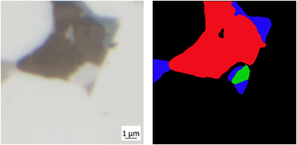
Left: 256 × 256 px RGB patch from the Fe₁₄Nd₂B-magnet image. Center: Mask in grayscale. Color assignments: light gray – oxide, white – Nd-rich, Eta – gray, black – matrix. Right: 4-channel image (combination of the RGB microstructure and mask).

3.3 Workflow for experiment execution

In order to effectively develop the study, it was structured as shown in Figure 4.

Figure 4:

Flow chart of the main experiment with the Fe₁₄Nd₂B-magnet dataset. For the other experiments, only the first three steps of this diagram were considered with minor variations, e.g. initial dataset, post-processing, etc.

With the BMQ training dataset, we trained the VQ-VAE and PixelCNN models to generate synthetic images of microstructures together with masks. The VQ-VAE model was trained to achieve the lowest reconstruction loss and to produce the z-matrices/codes in the embedding space, while the PixelCNN model was trained to learn the distribution of those matrices and generate new ones. Then, we decoded the generated matrices with the trained VQ-VAE decoder and split the resulting images into microstructure and mask.

To pre-test the quality of the synthetic images, we took the microstructural images to be inferred using the domain expert’s trained segmentation model. Once the model issued the masks, a visual comparison, with the synthetic ones, was carried out. The idea of this evaluation was to see if the two masks were similar; otherwise, we could assume that the synthetic images were of poor quality and that the model was to be retrained.

After the successful evaluation, starting from the initial datasets (Table 1) as a reference, we arranged new diverse datasets including different amounts of synthetic data to analyze how these data influence the predictions of the semantic segmentation models. For this purpose, 46 U-Net models were trained for a quantitative and qualitative analysis of the synthetic data. The U-Net models, from an architectural point of view, are the same (Table 3), only the datasets used for training are different.

Table 3:

Selected model hyperparameters for training the 46 U-Net models.

Hyperparameters	Value/name	Remark
Backbone	EfficientNetB3	–
Number of classes	4	The 3 phases and the matrix (red, green, blue and black).
Input shape	256 × 256 × 3	–
Initial weights	ImageNet	–
Epochs	200	With “EarlyStopping” to stop training when the IoU score did not improve after 15 epochs.
Steps per epoch	Not constant	Length of the train dataset divided by the batch size.
Validation steps	Not constant	Length of the validation dataset.
Batch size	2, 1	Train, validation.
Optimizer	Adam with LR = 0.001	With “ReduceLROnPlateau” callback in order to reduce
		the learning rate when the IoU did not improve after 5 epochs.
Compound loss function	Dice-focal (categorical)	–

4 Applied machine learning models

4.1 VQ-VAE: modifications and preliminary results for final datasets preparation

The implementation of this model was taken from [27] and adapted to the goal of this paper. The most prominent change in this work was the combination of the micrographs with the masks to be the input of the encoder, as in turn, the decoder was adjusted to provide an output of the same dimensions (Figure 5).

Figure 5:

Training scheme of VQ-VAE extracted from [6] and modified with the paper approach. The differences with respect to the original figure of Van Den Oord et al. [6] that can be seen in our figure are: K = 10, the 4-channel images as input and output and the matrix z containing values from 1 to 10.

Several tests were conducted to find the model hyperparameters that fit this approach and the main modifications (Table 4) with respect to the authors’ example were the following:

Table 4:

Modification of the model hyperparameters in the VQ-VAE model.

Hyperparameters	DeepMind [16]	Ours
Dataset and input shape (height, width, channels)	(32, 32, 3)	(256, 256, 4)
Number of images	60,000 (Cifar10)	62 (BMQ)
Batch size	32	8
D (embedding dimension)	64	64
K (embedding vectors)	512	10
Number of training updates	10,000	50,000

To train the model, we selected the BMQ dataset since we could not achieve favorable results with the SHQ. Of the 62 patches, 56 were part of the training and 6 for validation, then as the number of available images was much smaller than the original example from the authors, the batch size was reduced to 8.

Apart from that, since the selected images had 3 classes/phases and the background (matrix), the embedding vectors were significantly reduced, so that the PixelCNN model could learn the matrix distribution of the embedding space by a combination of a reduced number of vectors while the VQ-VAE decoder could still reconstruct good quality outputs (Figure 6), based on human perception.

Figure 6:

Top: 256 × 256 px original image and mask combined in a 4-channel image taken from the dataset. Bottom: 256 × 256 px reconstruction using the trained VQ-VAE model.

For an improvement in the reconstruction error (mean squared error) and the quality of the decoded output, we increased the training steps. In addition, the checkpoint was added to the source code, in order to save the model with the lowest reconstruction error based on the training dataset.

Step-by-step training of the model was followed by applying inference on an image from the validation dataset at every checkpoint. In Figure 7, it is shown that at the first checkpoint (step 100), the reconstruction was made up of horizontal and vertical lines, and almost no differentiation between the phases was visible.

Figure 7:

VQ-VAE training monitoring. From left to right: 1. Image from the validation dataset divided into microstructure and mask (the dataset does not contain scalebar) 2–4. Reconstructed images, at different steps of the training, with the corresponding reconstruction error.

Then at 12,000 steps, the model reconstructed the mask very poorly and some regions of the microstructure were not reconstructed. Finally, at the checkpoint at step 46,700, the model reached the best reconstruction, although there were some errors in the output mask, especially at phase edges due to errors in object boundaries in the original EDF images, e.g., blue pixels appearing at oxide boundaries, these did not preclude the aim of this study.

Figure 8 shows how the reconstruction error tends to decrease with time after each training step of the VQ-VAE model.

Figure 8:

VQ-VAE training plot. Reconstruction error on the training dataset.

4.2 PixelCNN: modifications and preliminary results for final datasets preparation

Once the VQ-VAE model was trained, we obtained the 62 z-matrices (Figure 9) composed with the codebook indices from the images of the BMQ dataset to train the PixelCNN model.

Figure 9:

Fe₁₄Nd₂B-magnet – representation of images in the trained embedding space. Left: Original microstructural images taken from the dataset. Center: Original masks taken from the dataset. Right: z-matrices composed with the 10 codebook indices. Each color represents an index of the codebook.

At the end of the PixelCNN training, a sampler model was built to generate new z-matrices from empty matrices. This model took empty matrices of 64 × 64 px as input and predicted each element based on pixels that are above and on the left of it. Then, using the VQ-VAE decoder, synthetic 4-channel images were generated. To better visualize them, in Figure 10 they were split into a microstructural image and mask.

Figure 10:

Fe₁₄Nd₂B-magnet – synthetic image generation. Left: Synthetic microstructural image. Right: Synthetic mask without post-processing.

At first glance, it can be seen that the masks were created correctly, but when observing the boundaries, different pixel values and not just one per class can be identified. This was the result of using poor quality images, so without processing, these masks could not be used directly in semantic segmentation models. To create useful masks for the U-Net, we processed the generated ones. First, we applied the k-means [28] algorithm to group the pixels into the 3 classes and the background; then, we filtered and removed small objects (<200 px²), and those regions were filled with the neighboring class (Figure 11).

Figure 11:

Step-by-step mask pre-processing for U-Net. Left: Synthetic generated mask. Center: Result from the k-means (4 clusters). Right: Result of filtering small objects and filling them with the correct class.

A quality pre-test was performed. Figure 12 shows the raw synthetically generated masks compared to the masks inferred by the subject matter model and it can be seen that both are similar, meaning that the model correctly predicted the synthetic objects.

Figure 12:

Fe₁₄Nd₂B-magnet – quality pre-test of synthetic images. Left: Synthetic microstructural image. Center: Synthetic mask without post-processing. Right: Mask inferred by the model of the expert.

4.2.1 Dataset preparation with addition of synthetic data for training semantic segmentation models

Table 5 illustrates the initial size of the training and validation datasets in the second column. The training datasets were increased with each value in the third column, while the validation one remained unchanged. The base datasets were based on those described in Table 1. The columns “Train/Val” and “Test” contain the number of real images, while the third column lists the percentages of synthesized images added to the training dataset with respect to the length of the base training datasets.

Table 5:

Prepared datasets for training the semantic segmentation models.

Dataset name	Train/val	Addition of synthetic data to the train dataset [%]	Test
SHQ	16/5	50, 75, 100, 150, 200, 250, 300	7 + 20
SLQ	16/5	50, 75, 100, 150, 200, 250, 300	27 (SHQ)
BLQ	48/12	50, 75, 100, 150, 200, 250, 300	27 (SHQ)
BMQ	48/12 (21 SHQ)	50, 75, 100, 150, 200, 250, 300	27 (SHQ)

1. BLQ and BMQ contains two images less than the initial datasets since they were discarded as no relevant phases were present (Figure 13). Patches with only matrix phase would introduce more class imbalance to the test dataset (Table 2).

For example, from the SHQ training dataset, an SHQ [50 %] dataset was created by adding 8 synthetic images (50 % of 16). In total, we formed 28 datasets with synthetic data from the initial 4, without synthetic images.

For a more extensive study, only synthesized data were used to create 14 more datasets by considering the size of the large datasets (Table 6). The validation datasets were composed only from original images with respect to BLQ and BMQ. As an example, the SyntLQ [50 %] and SyntMQ [50 %] consisted of the following: Training – 24 synthetic images, Validation – 12 real images (from BLQ and BMQ, respectively) and Test – 27 real images from SHQ.

Table 6:

Prepared datasets for training the semantic segmentation models.

Dataset name	Train/val	% training synthetic data	Test
SyntLQ	48/12	50, 75, 100, 150, 200, 250, 300	27 (SHQ)
SyntMQ	48/12 (21 SHQ)	50, 75, 100, 150, 200, 250, 300	27 (SHQ)

1. Training data is synthetic. Validation LQ and MQ are real images.

Figure 13:

Fe₁₄Nd₂B-magnet – images from the initial dataset that were discarded for training the semantic segmentation models since no relevant information was present.

In other words, the validation and test datasets remained unchanged and contained only real data, while the training datasets were purely synthetic. The values in the second column refer to SyntLQ [100 %] and SyntMQ [100 %].

4.3 U-Net for quantitative and qualitative analysis of generated images

We set up a Jupyter Notebook to train the U-Net architecture on each of the 46 datasets in the most equitable manner. The implementation from the GitHub repository [29] was adapted to this work. We kept all model hyperparameters constant (Table 3) and the only variation was the number of images that made up each dataset.

The purpose of training 46 models with the different datasets was to evaluate the metrics applied on the SHQ test dataset composed of 27 real images and to draw conclusions about the use of synthetic data in semantic segmentation models.

4.3.1 Missing Class IoU – a customized metric for model evaluation

In addition to the common metrics, we developed a personalized metric, “Missing Class IoU”, to evaluate the semantic segmentation models. The principle of this new metric is the same as the mIoU but it does not consider classes that are not part of the ground-truth mask when calculating the average IoU of all classes (C _n ).

(1) M i s s i n g C l a s s I o U = ∑ i n I o U C n n

Thus, in the case of the example given in Figure 14, the new metric is calculated as follows:

I o U Yellow + I o U Blue + I o U Background 3 = 1 + 1 2 + 32 34 3

Figure 14:

Example of a 6 × 6 px dummy image: Left: Ground-truth mask. Right: Result of a model prediction. The colors of the pixels refer to different classes.

For the yellow class, the intersection (TP) and union (TP + FP + FN) values are 1, since the pixel in the upper right corner is yellow in both images. In the case of the green class, the mask does not contain green pixels, so this class is discarded for calculation. In the case of the blue class, the intersection value is 1 and the union is 2 (TP = 1 and FP = 1). For the background class, which consists of a union value of 34 pixels (TP = 32 and FN = 2), the intersection is 32, since there are only 2 pixels that were incorrectly predicted. The IoU of each class is then calculated and averaged, discarding the green class.

As can be seen, the IoU of the green class is not considered, since there is no green object in the ground truth; however, the falsely predicted green pixel is considered as an incorrect value for the background class. The reason why we created this metric was because in some inferred masks we noticed some class pixels that were not in the ground-truth mask, due to the poor quality of the EDF image, which makes it impossible for the human to label. In the following section, one can see the use of this metric and how it performs correctly.

5 Results

From the evaluation of the 46 models prepared for the Fe₁₄Nd₂B-magnet experiment, we created different graphs to easily compare the results. As said before, the analysis should be focused on the use of the metric developed for this specific case, “Missing Class IoU”, however, the accuracy and mIoU graphs are also presented to explain the results in more detail and to emphasize the use of the customized metric.

The scatter plots in this section were constructed with the same test dataset but with different metrics. The plots take as lower x-axis the percentage of synthetic data in addition to the original data, in other words, the results of multiplying the second and third columns of Tables 5 and 6, while the top x-axis represents the absolute amount of training data in the purely synthetic datasets (SyntLQ and SyntMQ), which are the same values as the amount of synthetic data added to the larger datasets (BLQ and BMQ).

5.1 Analysis according to the percentage of synthetic data added

Figure 15 shows the evaluation of the accuracy on the different datasets. It can be seen that the values of nearly all the models (except purely synthetic) were between 97.5 % and 98 %, with 100 % being the maximum that could be reached. It can be observed that BQM [100 %] had the highest value with a little more than 98 % followed by the BMQ dataset with 50 % of synthetic data and the SHQ [250 %]. In the case of the models trained with purely synthetic data (brown bars with line pattern), the model with highest accuracy, 97.2 %, is the one with 36 synthetic images. On the other hand, the models with the worst accuracy were, in general, those of SyntMQ and especially BMQ [300 %] with a value of 91.4 %, which is not shown in the graph to better observe the others. Furthermore, this graph allows one to visualize the metric in terms of the base models (horizontal colored and stylized lines), without synthetic data, where it can be seen that BLQ (green solid line) and SHQ (blue dotted line) had similar values around 98 %.

Figure 15:

Evaluation of accuracy on the 46 datasets according to the percentage of synthetic data added. The y-axis corresponds to the accuracy in %, the lower x-axis to the addition, in percentage, of synthetic data to the training datasets and the upper x-axis to the number of synthetic images, in the training dataset, for purely synthetic datasets. Stylized, colored horizontal lines represent the accuracy of the base models (without addition of synthetic data) and each bar represents the accuracy of the models trained with addition of synthetic data. Note that BMQ [300 %] and SyntMQ [50 %] are not shown in the graph because their accuracy was less than 95 %.

In the mIoU graph (Figure 16), the values are distributed over a wider range than the accuracy graph, for example, for the BMQ (red bars with stars pattern), its range goes from 69 % mIoU with the base model (red dashed lines) to 82 % with the model trained with 50 % synthetic data. Furthermore, if BMQ [0 %] is excluded from the graph, the BMQ model with the lowest mIoU would be the one with 150 % synthesized data (mIoU = 70.5 %), while the one with the most synthesized data (300 %) has an mIoU of 71.6 %.

Figure 16:

Evaluation of mIoU on the 46 datasets according to the percentage of synthetic data added.

The plot also shows that, in some cases, the mIoU values of the models with pure synthetic data were higher than those of the models trained with combined data. Additionally, when 50 % synthesized data was added to the base models, both SLQ and SHQ had a decrease in their metrics, while the opposite happened to BLQ and BMQ.

After highlighting the main results generated by the above metrics, we carried out the analysis of the “Missing Class IoU” for each dataset and, in turn, the graphs of this metric for each class separately.

The main observations from Figure 17 are as follows:

1. By adding 50 % of synthetic data, except for the pure synthetic data, all the models improved.

2. The purely synthetic SyntLQ model with 24 images had a higher value (87.3 %) of the metric than the base SLQ model (86.1 %).

3. BMQ [100 %] had the best performance (91 %).

4. BMQ [300 %] had the worst performance (76.1 %), barely below SyntMQ [50 %].

5. SLQ [250 %] almost reached the best performance of SHQ (90.3 %) and the performance of both at [50 %] was similar (≈90 %).

6. All models (except the purely synthetic ones) achieved an improvement over the initial state in almost all datasets extended with synthetic data.

7. Models without synthetic data have a value of about 89 %, except for the SLQ with 86.1 %.

8. Models trained with purely synthetic data are located below all those combined with real and synthetic data.

Figure 17:

Evaluation of “Missing Class IoU” on the 46 datasets according to the percentage of synthetic data added.

5.2 Analysis per class/phase

We extracted the values from the “Missing Class IoU” for each phase to provide another point of view. For example, when analyzing the best model, BMQ [100 %], the metric improved for absolutely all classes compared to the base model, as can also be seen in the inferred images (Figure 18). Moreover, when all graphs are examined together (Figure 19), for all phases except Nd-rich, the models trained with purely synthetic data are below the others, for each different value of the x-axis.

Figure 18:

Fe₁₄Nd₂B-magnet – segmentation on five images from the test dataset. By column: 1. Original microstructural image; 2. Corresponding mask in RGB; 3. Segmented image with the BMQ base model overlapped to the original; 4. Segmented image with the BMQ model [150 %] overlapped to the original; 5. Segmented image with the BMQ model [300 %] overlapped to the original.

Figure 19:

Evaluation of “Missing Class IoU” per class/phase on the 46 datasets. Note that BMQ [300 %] and SyntMQ [50 %] are not shown in the “Evaluation of Eta” graph because their corresponding value for the metric were 0 % and 14.9 %.

In the case of the first graph, that of the matrix phase, one can see that the values are mostly compressed between 97 % and 98 % approximately, followed by the graph of the oxide phase evaluation, between 90.5 % and 92.5 %. Then there are those of Nd-rich with values lower than 85 % and Eta, with values below 80 %. Some low values are also observed (excluding models trained with purely synthetic data), for example, in the case of SLQ [0 %] compared to their respective models trained on synthetic data, and in the case of BMQ [300 %], on the evaluation of the matrix and Eta phases.

6 Discussion

Based on the results, it is possible to improve semantic segmentation models using synthetic data. This approach allows one to decrease the time consumption in labeling large datasets as well as populating small ones.

It could be seen why accuracy and mIoU should not be used in this specific experiment with Fe₁₄Nd₂B-magnet images. The first metric, mainly because almost all models had a value higher than 97.5 %; this would reflect that they were almost perfect, whereas this was not the case, as could be seen with the other metrics and the predicted images (Figure 18).

For the second metric, a clear case of its limitation in this analysis is, for example, the following. When comparing the mIoU values of the BMQ [150 %] and BMQ [300 %] models, the first intuition would be that the latter performed better than the former; however, when observing these predicted images again, it can be seen that the Eta phase was not detected for the latter model.

To validate the development of the “Missing Class IoU”, Figure 20 shows two clear examples with predicted masks using the BMQ model with 150 % and 300 % synthetic data. For the images in the first row, it can be seen that the results of the metrics are the same for both models, since all the values of each class are taken into account.

Figure 20:

Two examples to understand the “Missing Class IoU” metric. By column: 1. Original RGB mask 2. Mask predicted with the BMQ [150 %] model 3. Mask predicted with the BMQ [300 %] model.

However, in the second example, the difference is that the green class is not considered for the calculation of the image inferred by BMQ [150 %], so the sum of the IoU per class is divided by 2 and not by 3 (3 because the red class is not present). A final clarification on this situation is that, if someone does not see the inferred images and receives the information that the mIoU of an image is 65 %, one might think that the model has completely failed in its prediction, when, in fact, it has not.

In addition, if the BLQ and BMQ base models are compared with their respective ones by adding 50 % of synthetic data, the improvement is very large but this can be confirmed by looking at the inferred images by these models or plotting the mIoU of each image on a histogram, as something similar to the above may occur.

Although it is not clear how much data to generate and use, the combination of both original and synthetic data produces better models than both separately. Besides, this can be checked by generating a large amount of synthetic data, then training a few models by taking different percentages and observing the “Missing Class IoU” graph.

Thus, in the current analysis, the BMQ [100 %] model would be chosen, which has increased from 89.5 % to 91 % due to the addition of synthetic data. Figure 21 shows some inferred images by this model. Note that in case of other materials and approaches, the appropriate metric should be chosen for the selection of the best model.

Figure 21:

Segmentation on five images from the test dataset. By row: 1. Original microstructural image; 2. Corresponding mask in RGB; 3. Segmented image with the BMQ [100 %] model and overlapped on the original.

Moreover, the use of “per class/phase” graphs allows the analyst to observe poor inference in specific classes, commonly due to class imbalance or labeling errors in the datasets. In this way, synthetic images with more composition of the unbalanced class and more accurate masks can be added simultaneously.

Other conclusions can also be drawn from these graphs, e.g. the first two plots from Figure 19 (matrix, Eta) show that the evaluation is consistent, for instance, by checking the SLQ [0 %] and BMQ [300 %] which had the lowest values of their corresponding datasets. Both models had problems in differentiating the Eta phase from the Matrix.

On the other hand, the large improvement of SLQ with 50 % synthetic data was basically due to improved detection of the Eta phase, while the worsening of BMQ from 250 % to 300 % was due to the null detection of that phase.

Regarding the quality of the images, one aspect to note in the production of the 4-channel image is that, although the VQ-VAE and PixelCNN models are trained with the BMQ, which has several labeling errors, the synthetically produced masks have a high accuracy and show almost no pixel value errors. Whereas in reality, in most cases, there are no perfect masks for training (Figure 22).

Figure 22:

Fe₁₄Nd₂B-magnet image patch taken from the training dataset. The microstructural image has unsharp boundaries, variation of pixel colors due to EDF (blue pixels can be seen in the oxide phase) and a huge wrong label.

The important question to answer would be why the semantic segmentation models were improved with synthetic images, to which a possible answer would be the fact that the generated labels are more accurate. Although the generated microstructure does not look 100 % real, as described in the literature, labeling errors lead to a worse performance of the models.

When one creates a semantic segmentation model and its results are not as desired, the first thing to look at is the conditions of the masks. If these are correct, instead of acquiring more images and labeling them, it may be a great option to use the workflow explained in this paper, since on the same day one can train the set of models and generate synthetic images that could improve the segmentation, all much faster than the time needed in sample preparation, image acquisition and labeling, thus saving time and costly tasks.

One more point should be noted, which is that of data augmentation. Applying, for example, the Albumentations library [30] to augment the datasets requires specific domain knowledge. One must correctly define which image transformation operations can be used without altering the data in a way that hinders model generalization. As shown in the results section, incorrect selection of data augmentation can lead to worse performance (Missing Class IoU = 89.2 %) than not using data augmentation as in the base BMQ model (Missing Class IoU = 89.5 %).

Although with the correct application of data augmentation, a great performance could probably be achieved and maybe even better than BMQ [100 %], the application of the workflow of this paper does not involve a previous study of the images. In this case, there is no need to define what kind of augmentation to apply but only requires combining the real image with the mask and training the VQ-VAE model.

Depending on the distribution of the codes, it is the model that will be used to generate new codes; for example, during experimentation, PixelCNN has shown good results for non-uniform microstructures.

7 Limitations of the current workflow

Although the images generated for the experiment presented in this paper helped to improve the semantic segmentation models, they were not perfectly morphologically accurate and were somewhat blurred.

The former was due to the PixelCNN model, since the z-matrices obtained by the VQ-VAE model differentiated each phase well. Further experiments were performed with other materials, e.g., Li-ion battery microstructures, in which the microstructure layers are more clearly distributed, and the result of the PixelCNN model was poor, as it failed to learn the distribution of the layers.

The second problem is the reconstruction of blurred images due to the VQ-VAE model, which is explicitly shown in the authors’ paper.

8 Conclusion and outlook

In conclusion, we would like to highlight a few points:

1. Using the combination of both original and synthetic data results in improved performance (1–4%) of the semantic segmentation model compared to training with both separately.

2. The synthetically produced masks have well-defined object edges and barely show any over segmentation or misclassification of pixels, even if the models were trained with various labeling errors.

3. VQ-VAE exhibited good performance but should still produce less blurred images. PixelCNN is adaptable to approaches, where the phases are more sparsely distributed and not very adaptable in the case of densely concentrated regions, such as in a pattern form where the pixels are distributed in a structured way. Nevertheless, there are new versions of PixelCNN, that improve generation performance and overcome the “blind spot problem”, that can be tested for this workflow.

4. The proposed “Missing Class IoU” is useful for evaluation in cases where images have small objects that were not labeled but detected, and whose class is not part of the label. Thus, very low mIoU values are avoided.

5. “Per class/phase” graphs allow the analyst to observe poor inference in specific classes (e.g. 14.9 % on the evaluation of “Missing Class IoU” on Eta phase with SyntMQ [50 %]) and a more detailed understanding of the metrics used.

6. For a significant improvement of the workflow, it would be of interest to generate the dual synthetic image with the incorporation of variables in the latent space to be able to manipulate microstructural properties, e.g. phase fraction, in order to populate or balance datasets with the desired phase/property.

7. This approach would overcome a limitation of data augmentation, which focuses on creating new images by making global changes to the original image. The augmented data do not have semantic meaning and therefore, do not improve generalization ability of the semantic segmentation models when there is imbalance in different classes. Carrying out local changes or adding microstructural information in the latent space could overcome imbalance of specific classes.

References

[1] Cognilytica, AI Data Engineering Lifecycle Checklist, Washington, DC, Cognilytica White Paper, 2020.Search in Google Scholar
[2] A. Mumuni and F. Mumuni, “Data augmentation: a comprehensive survey of modern approaches,” Array, vol. 16, 2022, Art. no. 100258. https://doi.org/10.1016/j.array.2022.100258.Search in Google Scholar
[3] T. Ishiyama, T. Imajo, T. Suemasu, and K. Toko, “Machine learning of fake micrographs for automated analysis of crystal growth process,” Sci. Technol. Adv. Mater.:Methods, vol. 2, no. 1, pp. 213–221, 2022. https://doi.org/10.1080/27660400.2022.2082235.Search in Google Scholar
[4] T. Ishiyama, T. Suemasu, and K. Toko, “Semantic segmentation in crystal growth process using fake micrograph machine learning,” Sci. Rep., vol. 14, no. 1, 2024, Art. no. 19449. https://doi.org/10.1038/s41598-024-70530-3.Search in Google Scholar PubMed PubMed Central
[5] P. Isola, J. Zhu, T. Zhou, and A. Efros, “pix2pix2017: image-to-image translation with conditional adversarial networks,” CVPR, pp. 5967–5976, 2017.10.1109/CVPR.2017.632Search in Google Scholar
[6] A. Van Den Oord, O. Vinyals, and K. Kavukcuoglu, “Neural discrete representation learning,” Adv. Neural Inf. Process. Syst., vol. 30, pp. 6309–6318, 2017.Search in Google Scholar
[7] A. Van Den Oord, N. Kalchbrenner, O. Vinyals, L. Espeholt, A. Graves, and K. Kavukcuoglu, “Conditional image generation with pixelcnn decoders,” Adv. Neural Inf. Process. Syst., vol. 29, pp. 4797–4805, 2016.Search in Google Scholar
[8] O. Ronneberger, P. Fischer, and T. Brox, “U-net: convolutional networks for biomedical image segmentation,” in Medical Image Computing and Computer-Assisted Intervention – MICCAI 2015, Cham, Springer International Publishing, 2015, pp. 234–241.10.1007/978-3-319-24574-4_28Search in Google Scholar
[9] S. Chun, S. Roy, Y. T. Nguyen, J. B. Choi, H. S. Udaykumar, and S. S. Baek, “Deep learning for synthetic microstructure generation in a materials-by-design framework for heterogeneous energetic materials,” Sci. Rep., vol. 10, no. 1, 2020, Art. no. 13307. https://doi.org/10.1038/s41598-020-70149-0.Search in Google Scholar PubMed PubMed Central
[10] T. Hsu, W. K. Epting, K. H. H. W. Abernathy, G. Hackett, A. Rollett, P. A. Salvador, and E. A. Holm, “Microstructure generation via generative adversarial network for heterogeneous, topologically complex 3D materials,” JOM, vol. 73, no. 1, pp. 90–102, 2021. https://doi.org/10.1007/s11837-020-04484-y.Search in Google Scholar
[11] P. Trampert, D. Rubinstein, F. Boughorbel, C. Schlinkmann, M. Luschkova, P. Slusallek, T. Dahmen, and S. Sandfeld, “Deep neural networks for analysis of microscopy images—synthetic data generation and adaptive sampling,” Crystals, vol. 11, no. 3, p. 258, 2021. https://doi.org/10.3390/cryst11030258.Search in Google Scholar
[12] C. Shen, J. Zhao, M. Huang, C. Wang, Y. Zhang, W. Xu, and S. Zheng, “Generation of micrograph-annotation pairs for steel microstructure recognition using the hybrid deep generative model in the case of an extremely small and imbalanced dataset,” Mater. Charact., vol. 217, 2024, Art. no. 114407. https://doi.org/10.1016/j.matchar.2024.114407.Search in Google Scholar
[13] T.-C. Wang, M.-Y. Liu, J.-Y. Zhu, A. Tao, J. Kautz, and B. Catanzaro, “High-resolution image synthesis and semantic manipulation with conditional GANs,” in 2018 IEEE/CVF Conference on Computer Vision and Pattern Recognition (CVPR), Salt Lake City, UT, USA, 2018.10.1109/CVPR.2018.00917Search in Google Scholar
[14] D. Eschweiler, R. Yilmaz, M. Baumann, I. Laube, R. Roy, A. Jose, D. Brückner, and J. Stegmaier, “Denoising diffusion probabilistic models for generation of realistic fully-annotated microscopy image datasets,” PLoS Comput. Biol., vol. 20, no. 2, 2024, Art. no. e1011890. https://doi.org/10.1371/journal.pcbi.1011890.Search in Google Scholar PubMed PubMed Central
[15] T. Neff, C. Payer, D. Stern, and M. Urschler, “Generative adversarial network based synthesis for supervised medical image segmentation,” in Proceedings of the OAGM & ARW Joint Workshop 2017: Vision, Automation and Robotics, P. Roth, Ed., Graz, Technischen Universität Graz, 2017, pp. 140–145.Search in Google Scholar
[16] V. Thambawita, P. Salehi, S. A. Sheshkal, S. A. Hicks, H. L. Hammer, S. Parasa, T. de Lange, P. Halvorsen, and M. A. Riegler, “SinGAN-Seg: synthetic training data generation for medical image segmentation,” PLoS One, vol. 17, no. 5, 2022. https://doi.org/10.1371/journal.pone.0267976.Search in Google Scholar PubMed PubMed Central
[17] P. Andreini, S. Bonechi, G. Ciano, C. Graziani, V. Lachi, N. Nikoloulopoulou, M. Bianchini, and F. Scarselli, “Multi-stage synthetic image generation for the semantic segmentation of medical images,” in Artificial Intelligence and Machine Learning for Healthcare: Vol. 1: Image and Data Analytics, Cham, Springer International Publishing, 2023, pp. 79–104.10.1007/978-3-031-11154-9_5Search in Google Scholar
[18] T. Karras, T. Aila, S. Laine, and J. Lehtinen, “Progressive growing of GANs for improved quality, stability, and variation,” ICLR, 2018.Search in Google Scholar
[19] V. Fernandez, W. H. Lopez Pinaya, P. Borges, P.-D. Tudosiu, M. S. Graham, T. Vercauteren, and M. J. Cardoso, Can Segmentation Models Be Trained with Fully Synthetically Generated Data? Cham, Springer International Publishing, 2022, pp. 79–90.10.1007/978-3-031-16980-9_8Search in Google Scholar
[20] D. Saragih, A. Hibi, and P. Tyrrell, “Using diffusion models to generate synthetic labeled data for medical image segmentation,” Int. J. Comput. Assist. Radiol. Surg., vol. 19, no. 8, pp. 1615–1625, 2024. https://doi.org/10.1007/s11548-024-03213-z.Search in Google Scholar PubMed
[21] T. Salimans, A. Karpathy, X. Chen, and D. P. Kingma, “PixelCNN++: improving the PixelCNN with discretized logistic mixture likelihood and other modifications,” in International Conference on Learning Representations, 2017.Search in Google Scholar
[22] H. Rezatofighi, N. Tsoi, J. Gwak, A. Sadeghian, I. Reid, and S. Savarese, “Generalized intersection over union: a metric and a loss for bounding box regression,” in 2019 IEEE/CVF Conference on Computer Vision and Pattern Recognition (CVPR), Los Alamitos, CA, USA, 2019.10.1109/CVPR.2019.00075Search in Google Scholar
[23] S. Sugimoto, “Current status and recent topics of rare-earth permanent magnets,” J. Phys. D: Appl. Phys., vol. 44, no. 6, 2011, Art. no. 064001. https://doi.org/10.1088/0022-3727/44/6/064001.Search in Google Scholar
[24] B. J. Smith, M. E. Riddle, M. R. Earlam, C. Iloeje, and D. Diamond, Rare Earth Permanent Magnets: Supply Chain Deep Dive Assessment, United States, Office of Scientific and Technical Information, 2022.Search in Google Scholar
[25] A. Kini, A. Choudhary, D. J. A. Hohs, H. Baumgartl, R. Büttner, T. Bernthaler, D. Goll, and G. Schneider, “Machine learning-based mass density model for hard magnetic 14:2:1 phases using chemical composition-based features,” Chem. Phys. Lett., vol. 811, 2023, Art. no. 140231. https://doi.org/10.1016/j.cplett.2022.140231.Search in Google Scholar
[26] A. G. Valdecasas, D. Marshall, J. M. Becerra, and J. J. Terrero, “On the extended depth of focus algorithms for bright field microscopy,” Micron, vol. 32, no. 6, pp. 559–569, 2001.10.1016/S0968-4328(00)00061-5Search in Google Scholar PubMed
[27] G. DeepMind, “GitHub,” 2019 [Online]. https://github.com/deepmind/sonnet [accessed: Nov. 07, 2022].Search in Google Scholar
[28] E. W. Forgy, “Cluster analysis of multivariate data: efficiency versus interpretability of classifications,” Biometrics, vol. 21, no. 3, pp. 768–769, 1965.Search in Google Scholar
[29] J. M. Kezmann, “GitHub,” 2020 [Online]. Available at: https://github.com/JanMarcelKezmann/TensorFlow-Advanced-Segmentation-Models.Search in Google Scholar
[30] A. Buslaev, V. I. Iglovikov, E. Khvedchenya, A. Parinov, M. Druzhinin, and A. A. Kalinin, “Albumentations: fast and flexible image augmentations,” Information, vol. 11, no. 2, 2020, Art. no. 125. https://doi.org/10.3390/info11020125.Search in Google Scholar
© 2024 the author(s), published by De Gruyter on behalf of Thoss Media
This work is licensed under the Creative Commons Attribution 4.0 International License.
Articles in the same Issue
- Frontmatter
- Editorial
- AI in microscopy: shaping the future of imaging
- News
- Community news
- View
- AI-driven microscopy: from classical analysis to deep learning applications
- Research Articles