Optical sectioning in fluorescence microscopies is essential for volumetric measurements

1 Introduction

A conventional fluorescence microscope (CvFM) has no true optical sectioning capability [1]. Since the intensity of the fluorescence signal is proportional to the excitation intensity, it cannot provide an axial resolution. A confocal fluorescence microscope’s optical sectioning capability, i.e. its axial resolution, emerges from the proportionality of the fluorescence signal to the square of the excitation intensity [2].

Two-photon absorption fluorescence microscopy (TPA-FM) takes advantage of non-linear effects at high laser intensities, which allows fluorophores to be excited by low-energy photons [3], [4]. This method inherently incorporates optical sectioning since the excitation efficiency of fluorophores decreases away from the focus plane. A detection pinhole can be used (TPA-CFM) but is not required.

Confocal theta fluorescence microscopy (υ-CFM) [5], [6] introduces an innovative approach by employing two lenses arranged at a 90° azimuthal angle. The orthogonal overlap of point spread functions (PSF) significantly enhances the axial resolution, surpassing that of traditional confocal microscopy by at least a divisor three.

Ideally, these three methods observe a single location in space with sensors that provide no spatial resolution. They scan the object either along two or three dimensions and thus sample the specimen volume by volume, preferably with diffraction limited PSFs.

Light sheet-based fluorescence microscopy (LSFM) diverges from the epi-fluorescence arrangements by using two independently operated microscope objective lenses, arranged perpendicularly [7], [8], [9] and a camera in the sensor plane. High and low numerical apertures are used in the detection and in the illumination processes, respectively. This configuration creates a thin light sheet that exclusively illuminates the plane of focus, significantly reducing photobleaching and phototoxicity while discriminating against out-of-focus fluorescence. It achieves direct optical sectioning with drastically reduced energy exposure, rendering it ideal for recording many high-resolution, three-dimensional images of live specimens over long periods of time at high speed with regular cameras.

Light sheet-based fluorescence microscopes are also known as single/selective plane illumination microscopes (SPIM), digital scanned laser light sheet fluorescence microscopes (DSLM), and several other implementations.

These fluorescence microscopy techniques employ unique strategies for optical sectioning, with specific advantages but also challenges. CFM and TPA-FM provide foundational approaches. Theta- and light sheet-based instruments introduce innovative solutions for improved resolution and reduced specimen damage. This opens new possibilities for in-depth biological research with specimens that maintain their structural, morphological, and metabolic integrity.

2 Confocal fluorescence microscopy (CFM)

The confocal fluorescence microscope [10], [11] relies on two independent processes. A collimated laser beam is focused into a diffraction-limited single spot of light whose spatial extent is determined by the illumination point spread function. The emitted fluorescence light is collected with a point detector, whose spatial extent is also defined by a point spread function.

Since the two events: (1) excitation of a fluorophore, i.e. the absorption of a photon and the short-term storage of its energy by a molecule, and (2) detection of a fluorescence photon, i.e. upon emission of energy by the same molecule, are independent. The two processes can be described independently. Therefore, Figure 1 can be split into two parts (Figures 1 and 2).

Figure 1:

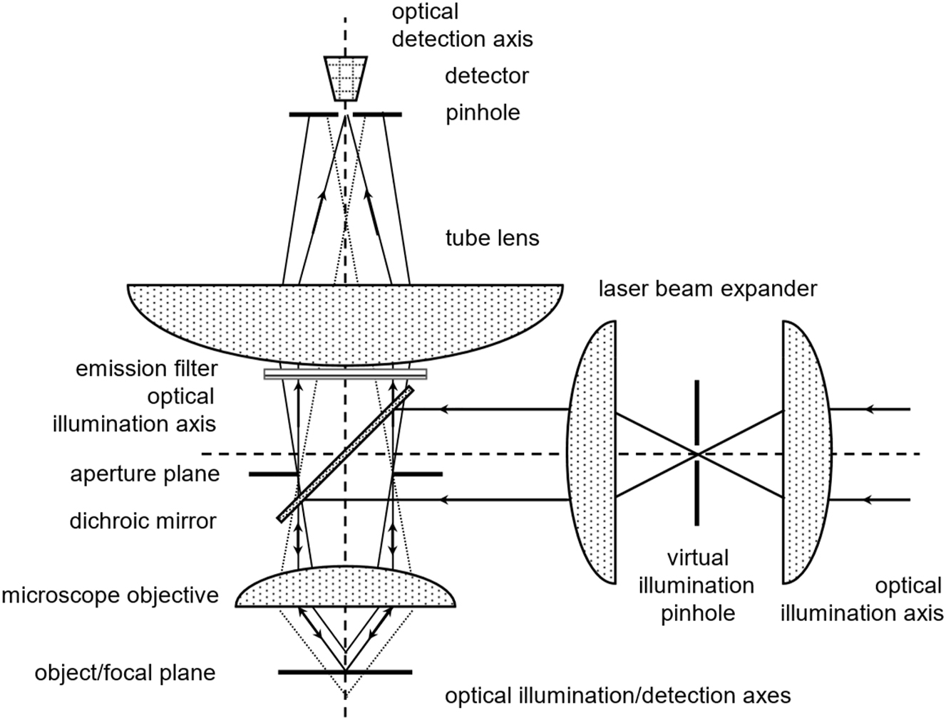
Canonic optical arrangement of a confocal epi-fluorescence microscope. The laser light enters the specimen from the right-hand side, is deflected by a dichroic mirror towards a microscope objective lens and forms a diffraction-limited spot of laser light in the focal plane. A fraction of the emitted fluorescence light is collected by the same lens, passes the dichroic mirror, and is focused by a tube lens into a pinhole in front of a detector. Light emitted centrally in the focal plane will pass the detection pinhole. Light emitted above or below the focal plane is expanded in the plane of the detection pinhole and will be partially discriminated. The excitation pinhole between the two lenses in the illumination train illustrates that the source as well as the sink of the photons are in conjugated locations.

Figure 2:

Path-independence illustration of a confocal epi-fluorescence microscope. Left: The laser light emanating from a collimated laser light source is deflected towards the objective lens by a dichroic beam-splitter. The objective lens focuses the light into the specimen in its focal plane. The excitation light passes the specimen and excites fluorophores within its path. The highest excitation intensity is in the focal plane. The area covered by the laser beam increases while the local intensity decreases as a function of the distance from the focal plane. Hence, fluorophores in front and behind the focal plane are excited but with location-dependent probabilities. Right: The fluorophores in the specimen emit in all directions, i.e. 4π, but only a segment is collected by the objective lens and focused into the pinhole in front of a detector by a tube lens. As indicated by the dashed lines, light emitted either in front or behind the focal plane is expanded in the image-/pinhole-plane. Only a portion will reach the detector. Please note, a confocal fluorescence microscope discriminates in the detection process.

Figure 3:

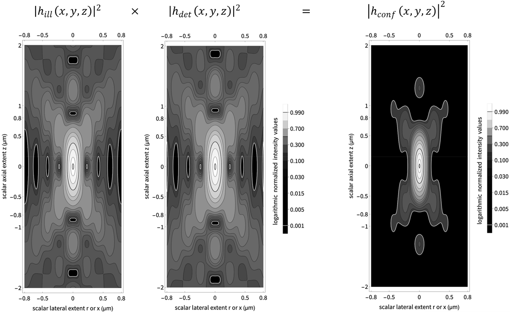
Calculating the confocal point spread function. The left figure shows a confocal illumination point spread function (PSF), the central figure a detection PSF, and the figure on the right their pixel-wise product, a confocal PSF. All PSFs are normalized to 1.0 in the origin (0.0, 0.0). The isophotes follow the values suggested in Born & Wolf figure 8.41. The black isophotes indicate the 50 percent transition. The white isophotes indicate the 1 permille transition. Hence, all areas contributing less than 1 permille are shown as black areas. Since the detection wavelength (520 nm) is longer than the illumination wavelength (488 nm), the detection PSF shows fewer undulations. The locations of the minima and maxima are similar but not identical.

Figure 4:

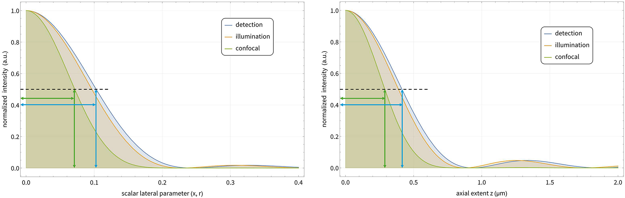
Characterizing lateral and axial extents of the PSFs. Both graphs show the meridional detection, illumination, and confocal intensity variations. The inserted lines indicate the locations of the FHWM of the illumination and detection PSFs. The respective ratios of the lateral and axial FWHM are about 1 / 2 .

Figure 5:

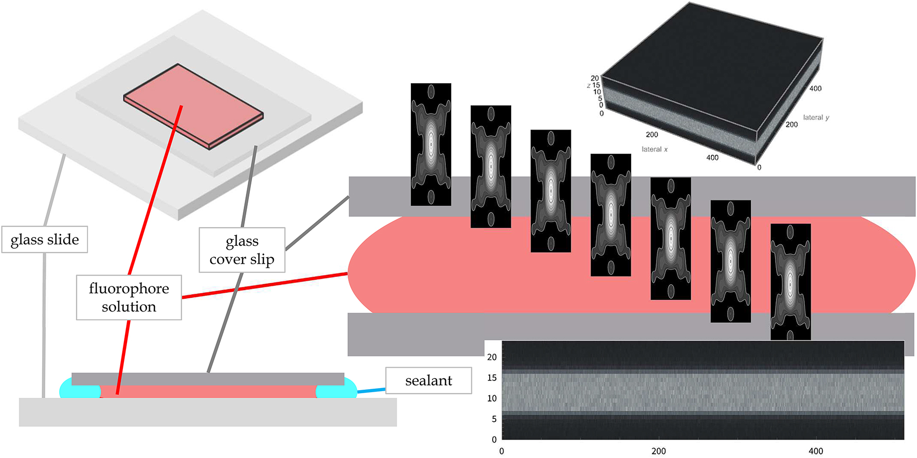
Measuring the optical sectioning capability of a confocal fluorescence microscope. Left: The specimen consists of a fluorescent oily or aqueous fluid, which is mounted between a cover slip and a glass slide and sealed to maintain its structural integrity. Center right: While recording a z-stack, i.e. using a feature available in every confocal fluorescence microscope, the probe enters and passes the fluid. Ideally, the signal will be dark, i.e. recorded inside the non-fluorescent cover slip, before it enters the fluid and dark again as it exits, as well as constantly bright while it passes through the fluid. This provides an excellent estimate of the background and the transitions from no-signal to signal to no-signal. Cover slips orthogonal to the axial movement of the lens allow the measurement around the axial edge and the calculation of signal averages and variances. Right top and bottom: An entire volume and an average image along a lateral axis show the glass, the fluorescent sea and the transition from glass to sea.

Figure 6:

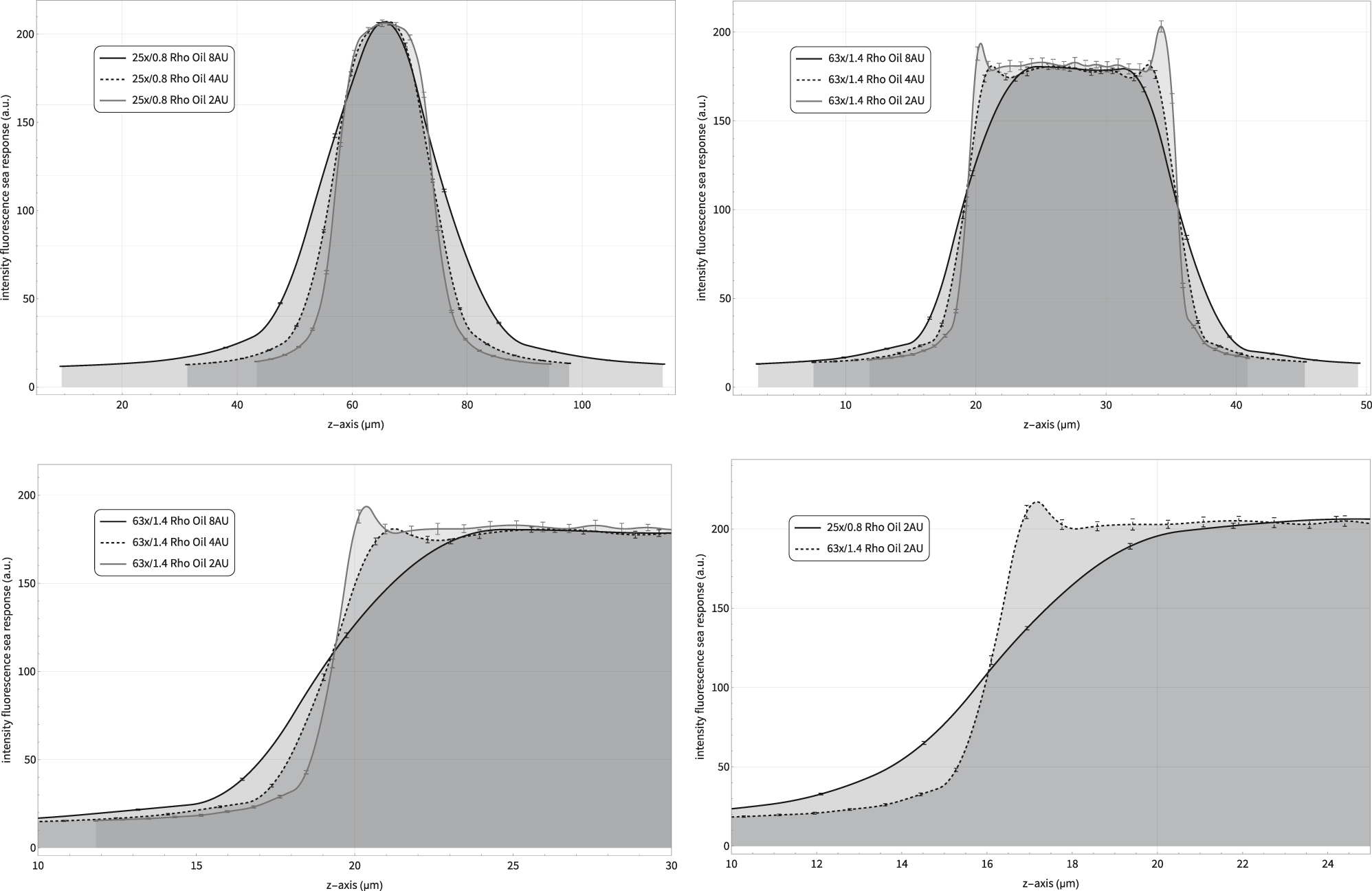
Sea responses of a confocal fluorescence microscope. The data are recorded with the same instrument but two different objective lenses and three different pinhole openings. Please note the different distances covered along the z-axes. Top left: Comparison of three responses with different pinhole settings. Smaller pinhole diameters result in steeper curves, i.e. better axial resolution. Top right: The same specimen observer with a higher NA lens. The two spikes only visible with 2 AU indicate that the confocality is not perfect. This is usually correctable by centering the pinhole. Bottom left: Response of the PSF entering the fluorescent sea. This information is usually sufficient. The first derivative would provide the axial PSF extents. Bottom right: A comparison of two different lenses. The considerably better axial resolution is evident as a higher steepness. The recording conditions are summarized in the short “Materials & Settings” section.

Figure 7:

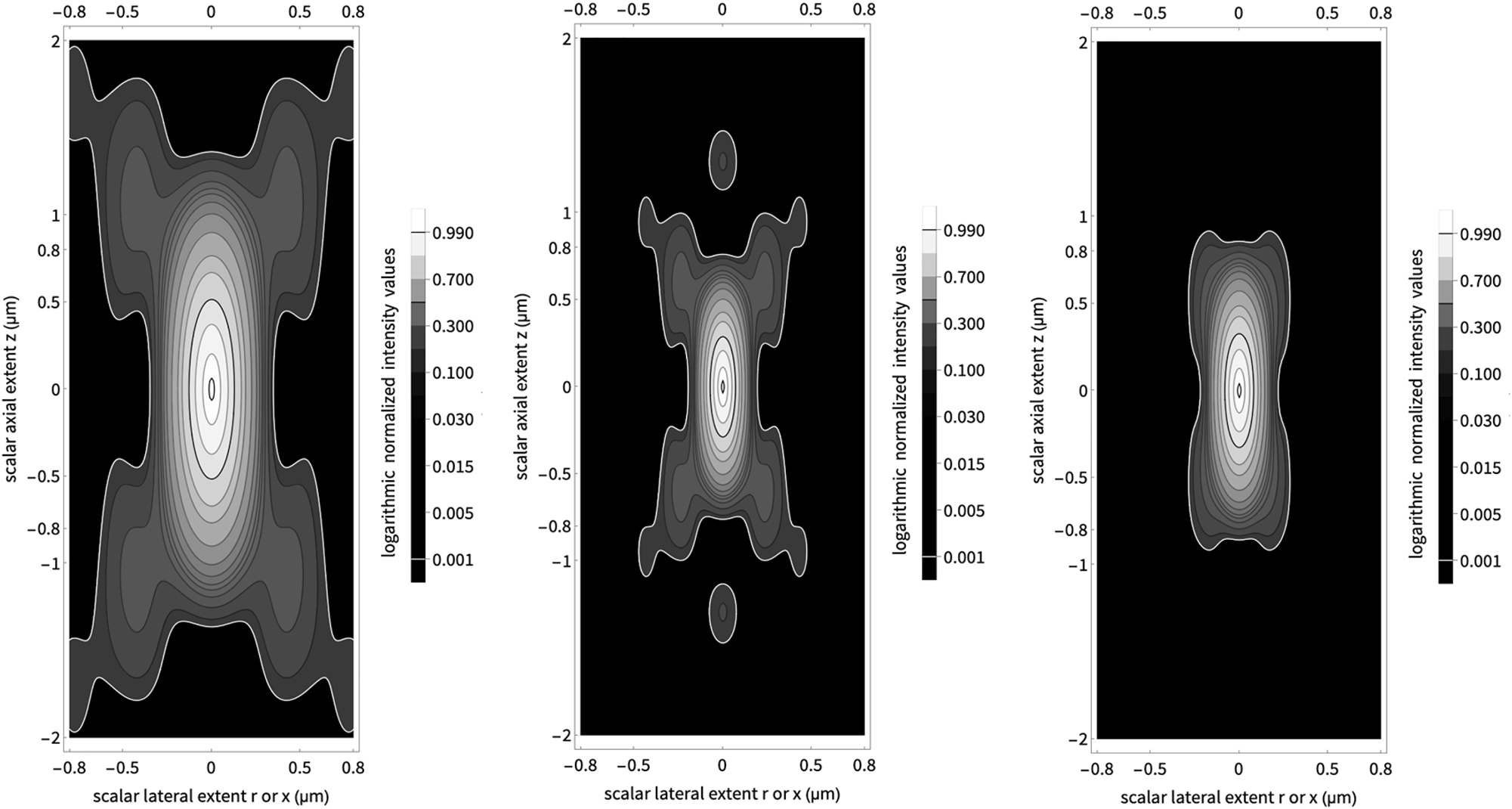
Comparison of point spread functions. The central part shows the PSF of a confocal microscope, the left part the PSF of a two-photon absorption microscope and the right part the PSF of a confocal two-photon absorption microscope, i.e. of a two-photon absorption fluorescence microscope plus a detection pinhole.

Figure 8:

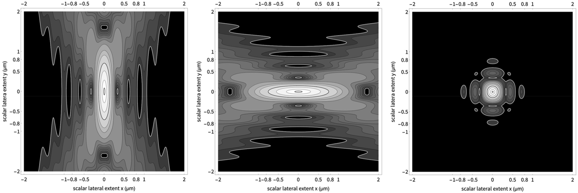
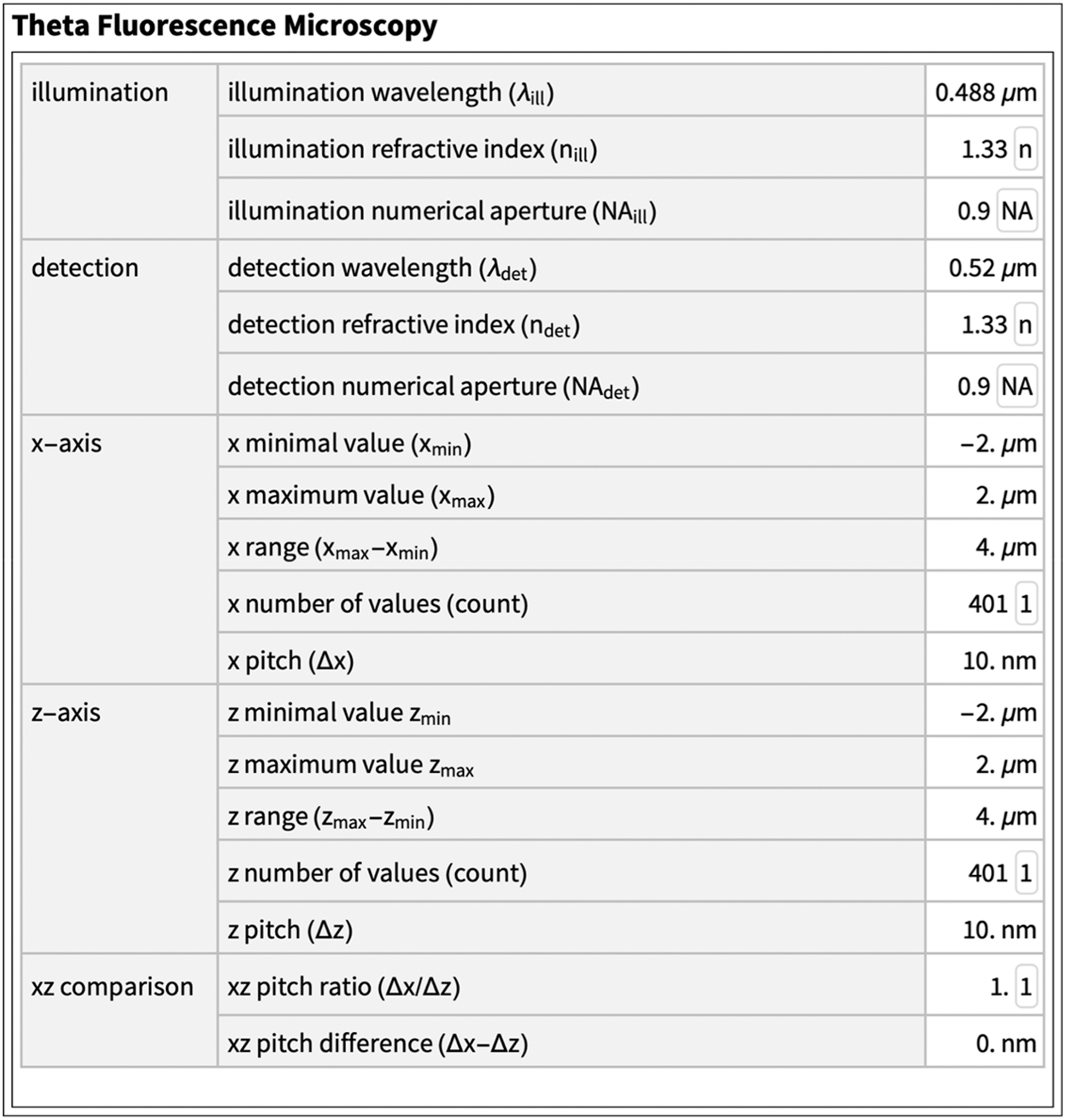
Point spread functions (PSF) of a confocal theta fluorescence microscope. The PSF on the right is the pixel-wise product of an illumination PSF and a detection PSF. Please note the use of water immersion lenses. The exact conditions are summarized below. The PSF is more like a sphere than an ellipsoid.

Figure 9:

Canonical setup of a light sheet-based fluorescence microscope. The illumination and detection lenses are perpendicular. The laser light is focused into the specimen with a low numerical aperture (NA) lens and forms a streak of light in the focal plane of the detection lens. The high NA detection lens collects the emitted light and forms an image in a camera. Please note, light sheet-based fluorescence microscopes discriminate in the illumination process.

One of the main disadvantages of the confocal fluorescence microscope sketched above is the relatively low speed of sequential spatial sampling. This is due to the movement of the common focal volume of the excitation and detection point spread functions relative to the specimen. Images of two- and three-dimensional fluorophore density distributions are constructed by software to form an image.

Another challenge in CFM is the exposure of the entire specimen to excitation light for each plane that is recorded along the optical axis. It results in a relatively high deposition of excitation energy. This in turn causes photo-induced damage, e.g. photobleaching and phototoxicity, which in turn prevent acquisitions of large 3D datasets and limit the observation of live specimens over extended periods of time.

Variants of confocal fluorescence microscopes that parallelize this process, e.g. spinning disk confocal fluorescence microscopes using cameras, suffer from a decreased axial resolution but will still work well with moderately thick specimens [12].

3 Calculating optical point spread functions

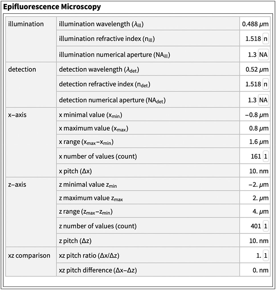
The basis for all calculations and figures presented in this paper is derived in [13]“ ‘Principles of Optics’ (1st edition 1959, 6th edition 1980) Pergamon Press Oxford” in § 8.8, formulas (11, 12). This section explains how to calculate the electromagnetic field U in terms of generalized coordinates v and u, which, respectively, extend laterally and axially. This approach is sufficient for small angular apertures (AA) and often referred to as a small angle approximation. The numerical aperture (NA) is the product of the angular aperture and the refractive index of the immersion medium. Hence, the Born & Wolf approximation (BWA) serves the purpose of this paper even for numerical apertures above 1 Equation (1).

Equation (1) reproduces the BWA. The two functions are identical but ordered slightly differently. The integral on the right summarizes the impact of the aperture and depends on u and v, which provide the location of a point in space. In this case, the illumination intensity is uniform and not interfered with by phase plates. The first factor in front of the integral weights the impact of the axial distance from the focal plane and the opening angle α, it does not depend on v. Finally, the wavelength λ/n, i.e. the ratio of the vacuum wavelength and the refractive index of the medium, scales the function. Neither the wavelength nor the refractive index appears anywhere else. This formula must be applied to each location of interest in the vicinity of the focus to return a complex value, i.e. the local amplitude and relative phase of the electromagnetic field. This amounts to around 100 K complex numbers in two dimensions and around 10 M complex numbers in three dimensions Equation (2).

The relationships between the generalized coordinates v and u and the physical properties of an optical device are used directly to calculate PSFs of ideal microscopes (§ 8.8.1 formula 4) Equation (3).

The function h returns the amplitude, i.e. a complex value, at a well-defined location. The product of h and its complex conjugate h* returns the intensity, i.e. a real number. This is indicated by the two bars and the square, i.e. the superscripted number 2. The intensity is used to calculate the power and the energy in a volume.

In a conventional fluorescence microscope, the function h x , y , z 2 provides a linear response in the sense that the intensity of the fluorescence emission is proportional to the intensity of the excitation signal.

Most interestingly, the intensity distribution can also be interpreted as a probability density function (PDF), which calculates the probability of locating a photon that has passed a pinhole in a specified volume. However, while PDFs are normalized by the total event space and PSFs by their maximum, they differ only by a constant Figure 3.

Hence, the function h x , y , z 2 provides the PSF as well as the PDF of a conventional widefield fluorescence microscope.

Since the two required events: (1) excitation of a fluorophore and (2) detection of a fluorescence photon are independent, the two point spread functions are multiplied Equation (4).

The detected fluorescence intensity in a confocal fluorescence microscope is thus essentially dependent on the square of the excitation intensity Figure 3.

It is important to understand what independent events infer. For example, when one throws a single cubic dice, the probabilities for either face pointing upwards is 1/6. When one throws two dice the probability for each pair is 1 / 6 × 1 / 6 = 1 / 6 2 . The probabilities are simply multiplied. Phrased differently, two events must occur (1) the excitation of a fluorophore and (2) the detection of a photon emitted by the same fluorophore. In a binary world this is the application of a logic AND, which is only true or equal to one if both inputs are true/one. In the real world, probabilities are multiplied.

The same procedure can be applied when quantifying the properties of an imaging device, e.g. a microscope objective lens. We know that (1) a microscope objective lens spreads or smears out the image of a point source, (2) a microscope objective in a confocal fluorescence microscope images two pinholes, i.e. one behind the light source and one in front of a detector, and (3) absorption and emission operate independently. Hence, we calculate a system point spread function by multiplying the probabilities for (1) absorbing an excitation photon in a certain location and for (2) detecting a fluorescent photon emanating from the same location.

The point spread functions are characterized by analyzing the central lateral and axial intensity distributions. A characteristic value is the full width at half of the maximum (FWHM), but a drop of the maximal intensity to the fractions 1/e or 1/e ² are also common Figure 4.

Although the lateral and axial extents of the PSF of a confocal fluorescence microscope are about 1.4× better than those of a conventional wide-field fluorescence microscope this does not mean that the increase can be taken advantage of [14] and results in an easily visible resolution improvement. The reason is the usually low signal to noise ratio, which is discussed in the paper referenced above. Furthermore, and very important, the improved lateral and axial resolutions do not explain the property of optical sectioning.

4 Optical sectioning

Optical sectioning refers to the axial resolution in microscopy. This means that one can distinguish different objects or a gap in between objects along the optical axis. However, as pointed out above, in a conventional fluorescence microscope the fluorescence emission intensity is directly proportional to the excitation intensity. This means, since the total, i.e. integrated excitation energy measured in any plane along the optical axis is identical, the emission intensity must also be constant. This is the physical-mathematical proof that a conventional fluorescence microscope lacks true optical sectioning and provides no axial resolution Equation (5).

One can also conclude that a non-linear response, e.g. the quadratic response encountered in confocal fluorescence microcopy will not be constant but rather vary along the optical axis Equation (6).

This resembles the point spread function of a two-photon absorption microscope Equation (7) intensities [3].

However, the excitation wavelength in a TPA-FM is up-to two times longer compared to the typical wavelengths used in single-photon fluorescence microscopy. Hence, its lateral resolution is worse than in a conventional microscope and its axial resolution is 2 ≅ 1.4 × worse than in a confocal fluorescence microscope.

5 Quantifying optical sectioning and axial resolution

A valid question is of course, how does one measure the axial resolution? In general, resolution refers to the capability of an optical instrument to separate two specimens. In this case, to separate two fluorescent beads, two thin fluorescent parallel lines or two thin fluorescent planes. This is directly possible but precise measurements will certainly suffer from severe photobleaching Figure 5.

A simple and straightforward method is to create an axial edge by mounting a small amount of a fluorescent dye dissolved in an oily or aqueous fluid between a cover slip and a glass slide [15].

The sea response is the integral over the entire PSF and the integral over the fraction of the confocal point spread function that is in contact with the fluorescent sea Equation (8). It is a cumulative function Figure 6.

Ideally, an x/z-image of this test specimen provides the intensities of a PSF entering and exiting this fluorescent sea. The derivatives of this cumulative or integrated signal provide axial extents, which are not shown.

6 Two-photon fluorescence microscopy

A two-photon fluorescence microscope takes advantage of non-linear resonant effects that are always present but only become apparent at high laser intensities [3], [16]. Fluorophores can be efficiently excited with two lower energy (higher wavelength) photons. Since essentially two independent events must take place during the excitation process, the illumination point spread function is squared. The net effect is an optical sectioning capability that is defined in the excitation process. This has the interesting property that, in contrast to conventional and confocal microscopy, fluorophores above or below the plane of focus are excited less. A detection pinhole is not required for the optical sectioning. The location, from which the emitted fluorescence light stems is defined in the excitation process, therefore, relatively large detectors can be used to efficiently collect the light from the specimen. This is often referred to as non-de-scanned detection Figure 7.

However, the required laser powers are usually significantly higher than in single-photon confocal fluorescence microscopy. In contrast to common believe, the resolution of a two-photon fluorescence microscope is not only considerably worse than that of a single-photon confocal fluorescence microscope but also worse than the resolution of a conventional fluorescence microscope.

A two-photon fluorescence microscope can be equipped with a detection pinhole. However, such a confocal two-photon fluorescence microscope collects an order of magnitude less signal and will still not perform as well as a comparable single-photon confocal fluorescence microscope. Unluckily, such a setup is required for a 4Pi(A) confocal fluorescence microscope [17], [18], [19] to dampen the side-lobes Equation (9).

While it is accurate that longer wavelengths generally provide less resolution, it is essential to clarify that two-photon microscopy allows for deeper tissue penetration due to less scattering of higher wavelengths, which is a significant advantage in certain biological applications. The trade-off in resolution is often considered acceptable due to these benefits.

7 Confocal theta fluorescence microscopy (υ-CFM)

A confocal epi-fluorescence microscope uses the same lens for the excitation of a fluorophore and the collection of the fluorescence emission. It has essentially the same properties as a confocal dia-fluorescence microscope that would use two opposing lenses in a collinear fashion for the excitation and the subsequent collection of the fluorescence emission.

A confocal theta fluorescence microscope uses two lenses that are arranged at an azimuthal angle υ of 90°. One lens is used in the excitation path and the other lens is used in the detection path [20], [21]. The two point spread functions can be treated very much like in a confocal fluorescence microscope. However, they do not overlap collinearly but orthogonally. This has the amazing effect that the point spread function is almost spherical. In particular, the axial resolution is dramatically improved by factors of three to ten over that of confocal fluorescence microscopes, depending on the numerical apertures of the involved objective lenses Figure 8.

It is fair to claim that a confocal theta fluorescence microscope beats the diffraction limited resolution of conventional and confocal fluorescence microscopes Equation (10).

A disadvantage that confocal theta fluorescence microscopy shares with all other sampling (scanning) devices is the low speed. However, since two lenses are used in the azimuthal arrangement confocal theta fluorescence microscopes can be massively parallelized at the expense of its optical sectioning capability.

8 Light sheet-based fluorescence microscopy (LSFM)

In contrast to a conventional or a confocal epi-fluorescence arrangement, a light sheet-based fluorescence microscope uses at least two independently operated lenses [22]. The lenses used for the excitation of the fluorophores are arranged at an angle of 90° relative to those used for the collection of the emission from a three-dimensional fluorophore density distribution. However, the field of view of the illumination lens is not fully illuminated, only a single line along the lateral axis that overlaps with the focal plane of the detection lens is utilized. In consequence, only a thin planar section centered on the focal planes of the detection lenses receives any light. The volume outside this light sheet is not illuminated and, therefore, the fluorophores outside the light sheet are not excited [7], [8], [23]. These fluorophores suffer less from photo-bleaching, contribute less to any phototoxic effects, and cannot emit any photons that would add to image blur Figure 9.

While light sheet-based fluorescence microscopy reduces photobleaching and phototoxicity significantly, it is not free from these effects. It’s crucial to note that any form of light exposure can will cause some kind of photodamage, especially during long-term imaging sessions.

The optical sectioning capability in a confocal fluorescence microscope stems from the combination of point illumination and point detection and suffers from the fact that the excitation light passes through the object and that the entire specimen is illuminated once for each plane that is recorded. The recording of a few hundred planes will invoke an excitation process for each fluorophore a few hundred times.

The optical sectioning in a light sheet-based fluorescence microscope is direct and only affects the fluorophores in the single plane that is illuminated and observed. Therefore, the energy required to record a three-dimensional stack of images with a light sheet-based fluorescence microscope is reduced by two to four orders (!) of magnitude relative to conventional and confocal fluorescence microscopy. Since modern cameras can be used to record millions of pixels in parallel, tens to hundreds of images with cellular resolution can be recorded within a few seconds e.g. [23].

The main two canonical means to create light sheets are: (1) A cylindrical lens in the illumination beam path, which focuses a collimated laser beam along one direction and forms a static light sheet [7], [8], [24]. (2) A galvanometer that tilts a collimated laser beam along one direction and forms a dynamic light sheet. The latter method produces beams of higher quality and can also be used in conjunction with annular apertures (e.g. Bessel-type, [25]) and two-photon excitation.

In abstract terms a light sheet-based fluorescence microscope is essentially a wide-field version of the theta fluorescence microscope.

Light sheet-based fluorescence microscopy has been extremely successful in the biological sciences in general and in developmental biology in particular. State-of-the-art dynamic three-dimensional in toto imaging would have never become possible if light sheet-based fluorescence microscopy had not provided the means to reduce the energy exposure by several orders of magnitude. It is now possible to generate three-dimensional stacks of optically sectioned images consisting of several million pixels with a high dynamic range of the same object along multiple directions several thousand times per day.

The application of light sheets lacking diffraction limited lasers has been mentioned several times in the literature during the past century (see [22]). However, the first laser light sheet-based fluorescence microscopes, i.e. an instrument that uses microscope objective lenses to generate high resolution images has first been built at EMBL [7], [8], [24]. The optical properties of all light sheet-based fluorescence microscopes are described with the theory developed to describe confocal theta fluorescence microscopy.

9 Outlook

The biggest challenge in all microscopic techniques is sample preparation. Most of the time is spent with arranging and mounting the specimen as well as processing and analyzing the data. The time spent in front of the microscope is usually short.

In volumetric measurements with fluorescence microscopes sample preparation depends on whether the specimen is dead or alive, on the number on fluorophores, the duration of the experiment, … Of course, not every possible aspect has to addressed in each experiment, but it is important to have an arsenal of options at one’s disposal. Particularly interesting are various tissue clearing and expansion techniques that are very well suited for optical sectioning in thick specimens [26].

On the instrumentation side one needs to keep an eye on Lattice light-sheet microscopy [27], [28], which bridges the gap between optical sectioning and super-resolution [29]. Adaptive optics has been demonstrated to work well in fluorescence light microscopy [30] since it has the potential to address specific optical aberrations due to the properties of the specimen as well as the observation depth.

Software tools such as DeconvolutionLab2 illustrate the importance of computational methods in enhancing the quality of optical sectioning images [31].

10 Summary

This paper details the advancements and methodologies in fluorescence microscopy, particularly emphasizing the critical technique of optical sectioning. Microscopes that take advantage of this technique are pivotal for visualizing and analyzing three-dimensional structures in specimens with high resolution. They significantly benefit scientific fields like cellular and developmental biology.

Mathematical models and equations are used superficially to describe the light–matter interactions in these microscopies, based on principles outlined in the foundational optics literature by Born & Wolf. The paper describes how to calculate point spread functions (PSFs) and discusses how optical sectioning capabilities are quantified through these mathematical frameworks. A particular emphasis is placed on regarding PSFs as proportional to probability density functions (PDFs), which helps to understand the broader idea of optical sectioning while simplifying the calculation of PSFs that operate with multiple microscope objective lenses.

Using the concepts of integrated intensities and sea responses the paper outlines how to measure the axial resolution of a confocal fluorescence microscope and how to cope with the unavoidable photo bleaching.

The paper reflects on the evolution of fluorescence microscopy, attributing advancements to ongoing research and collaboration in the field. The optical sectioning techniques discussed not only enhance imaging capabilities but also open new avenues for research by allowing scientists to observe biological processes in unprecedented detail.

11 Acknowledgements

The insights described in this paper have developed during the past almost fifty years, essentially during the evolution of deconvolution and confocal fluorescence microscopy pushed by, amongst many others, John Sedat, David Agard, Tziki Kam, Colin Sheppard, Tony Wilson, Ingmar Cox, Fred Brakenhoff, and James Pawley. Particularly important were developments in the laboratory of Roelof W. Wijnaendts-van-Resandt at EMBL (Heidelberg). I am grateful to my current and former students as well as collaborators at the European Molecular Biology Laboratory and at the Goethe-Universität Frankfurt am Main for the endless discussions and activities that are required to develop fundamental insight into scientific and technical topics.

Francesco Pampaloni and Daniel Constantin were so kind to check the manuscript and the references.

11 Materials & settings

The values and units used in this paper are summarized in two tables. The sea responses were recorded under the following conditions. dye: Rhodamine B (λ _ex = 553 nm, λ _em = 627 nm), specimens: ethanol-Rhodamine solution in oil, laser: excitation 514 nm, power 10.0 [%], GaAsP-detector: 526 nm–695 nm, image recording: scan speed 8, line averaging 4, frame size 512 × 512, zoom 8.0, Zeiss LSM 780, lenses: LD LCI Plan-Apochromat 25×/0.8, Imm corr DIC M27 setting oil, Plan-Apochromat 63×/1.4 Oil DIC M27. AU refers to AU settings as defined by Zeiss, z-interval and pixel size as suggested by Zeiss.

References

[1] D. A. Agard and J. W. Sedat, “Three-dimensional architecture of a polytene nucleus,” Nature, vol. 302, no. 5910, pp. 676–81, 1983. https://doi.org/10.1038/302676a0.Suche in Google Scholar PubMed
[2] I. J. Cox, “Scanning optical fluorescence microscopy,” J. Microsc., vol. 133, no. Pt 2, pp. 149–54, 1984. https://doi.org/10.1111/j.1365-2818.1984.tb00480.x.Suche in Google Scholar PubMed
[3] W. Denk, J. H. Strickler, and W. W. Webb, “Two-photon laser scanning fluorescence microscopy,” Science, vol. 248, no. 4951, pp. 73–6, 1990. https://doi.org/10.1126/science.2321027.Suche in Google Scholar PubMed
[4] F. Helmchen and W. Denk, “Deep tissue two-photon microscopy,” Nat. Methods, vol. 2, no. 12, pp. 932–40, 2005. https://doi.org/10.1038/nmeth818.Suche in Google Scholar PubMed
[5] S. Lindek, C. Cremer, and E. H. K. Stelzer, “Confocal theta fluorescence microscopy with annular apertures,” Appl. Opt., vol. 35, no. 1, pp. 126–30, 1996. https://doi.org/10.1364/AO.35.000126.Suche in Google Scholar PubMed
[6] S. Lindek and E. H. Stelzer, Confocal Theta Microscopy and 4Pi-Confocal Theta Microscopy, C. J. Cogswell and K. Carlsson, Eds., USA, SPIE (Society of Photo Optical Engineers), 1994, pp. 188–94.10.1117/12.172093Suche in Google Scholar
[7] J. Huisken, J. Swoger, F. Del Bene, J. Wittbrodt, and E. H. K. Stelzer, “Optical Sectioning Deep Inside Live Embryos by Selective Plane Illumination Microscopy,” Science, vol. 305, no. 5686, pp. 1007–9, 2004. https://doi.org/10.1126/science.1100035.Suche in Google Scholar PubMed
[8] J. Huisken, J. Swoger, F. Del Bene, J. Wittbrodt, and E. H. K. Stelzer, “Optical sectioning deep inside live embryos by selective plane illumination microscopy,” Science, vol. 305, no. 5686, pp. 1007–9, 2004. https://doi.org/10.1126/science.1100035.Suche in Google Scholar
[9] A. H. Voie, D. H. Burns, and F. A. Spelman, “Orthogonal-plane fluorescence optical sectioning: three-dimensional imaging of macroscopic biological specimens,” J. Microsc., vol. 170, no. Pt 3, pp. 229–36, 1993. https://doi.org/10.1111/j.1365-2818.1993.tb03346.x.Suche in Google Scholar PubMed
[10] J. B. Pawley, Ed., Handbook of Biological Confocal Microscopy, US, Springer, 1995.10.1007/978-1-4757-5348-6Suche in Google Scholar
[11] E. H. K. Stelzer, “The Intermediate Optical System of Laser-Scanning Confocal Microscopes,” in Handbook of Biological Confocal Microscopy, J. B. Pawley, Ed., US, Springer, 1995, pp. 139–54.10.1007/978-1-4757-5348-6_9Suche in Google Scholar
[12] R. Juskaitis, T. Wilson, M. A. Neil, and M. Kozubek, “Efficient real-time confocal microscopy with white light sources,” Nature, vol. 383, no. 6603, pp. 804–6, 1996. https://doi.org/10.1038/383804a0.Suche in Google Scholar PubMed
[13] M. Born and E. Wolf, Principles of Optics, Oxford, Pergamon Press, 1980.Suche in Google Scholar
[14] E. H. K. Stelzer, “Contrast, resolution, pixelation, dynamic range and signal‐to‐noise ratio: fundamental limits to resolution in fluorescence light microscopy,” J. Microsc., vol. 189, no. 1, pp. 15–24, 1998. https://doi.org/10.1046/j.1365-2818.1998.00290.x.Suche in Google Scholar
[15] R. W. Wijnaendts-Van-Resandt, H. J. B. Marsman, R. Kaplan, J. Davoust, E. H. K. Stelzer, and R. Stricker, “Optical fluorescence microscopy in three dimensions: microtomoscopy,” J. Microsc., vol. 138, no. 1, pp. 29–34, 1985. https://doi.org/10.1111/j.1365-2818.1985.tb02593.x.Suche in Google Scholar
[16] E. H. K. Stelzer, et al.., “Nonlinear absorption extends confocal fluorescence microscopy into the ultra-violet regime and confines the illumination volume,” Opt. Commun., vol. 104, nos. 4–6, 1994. https://doi.org/10.1016/0030-4018(94)90546-0.Suche in Google Scholar
[17] S. W. Hell, S. Lindek, and E. H. K. Stelzer, “Enhancing the axial resolution in far-field light microscopy: Two-photon 4Pi confocal fluorescence microscopy,” J. Mod. Opt., vol. 41, no. 4, 1994. https://doi.org/10.1080/09500349414550701.Suche in Google Scholar
[18] S. W. Hell, E. H. K. Stelzer, S. Lindek, and C. Cremer, “Confocal microscopy with an increased detection aperture: Type-B 4Pi confocal microscopy,” Opt. Lett., vol. 19, no. 3, pp. 222–4, 1994. https://doi.org/10.1364/OL.19.000222.Suche in Google Scholar PubMed
[19] S. W. Hell and E. H. K. Stelzer, “Fundamental improvement of resolution with a 4Pi-confocal fluorescence microscope using two-photon excitation,” Opt. Commun., vol. 93, nos. 5–6, pp. 277–82, 1992. https://doi.org/10.1016/0030-4018(92)90185-T.Suche in Google Scholar
[20] S. Lindek, E. H. K. Stelzer, and S. W. Hell, “Two New High-Resolution Confocal Fluorescence Microscopies (4Pi, Theta) with One- and Two-Photon Excitation,” in Handbook of Biological Confocal Microscopy, J. B. Pawley, Ed., US, Springer, 1995, pp. 417–30.10.1007/978-1-4757-5348-6_26Suche in Google Scholar
[21] E. H. K. Stelzer and S. Lindek, “Fundamental reduction of the observation volume in far-field light microscopy by detection orthogonal to the illumination axis: confocal theta microscopy,” Opt. Commun., vol. 111, nos. 5–6, pp. 536–47, 1994. https://doi.org/10.1016/0030-4018(94)90533-9.Suche in Google Scholar
[22] E. H. K. Stelzer, et al.., “Light sheet fluorescence microscopy,” Nat. Rev. Methods Primers, vol. 1, no. 1, 2021. https://doi.org/10.1038/s43586-021-00069-4.Suche in Google Scholar
[23] P. J. Keller and E. H. K. Stelzer, “Digital scanned laser light sheet fluorescence microscopy,” Cold Spring Harb. Protoc., vol. 2010, no. 5, 2010, Art. no. pdb.top78. https://doi.org/10.1101/pdb.top78.Suche in Google Scholar PubMed
[24] K. Greger, J. Swoger, and E. H. K. Stelzer, “Basic building units and properties of a fluorescence single plane illumination microscope,” Rev. Sci. Instrum., vol. 78, no. 2, 2007. https://doi.org/10.1063/1.2428277.Suche in Google Scholar PubMed
[25] F. O. Fahrbach and A. Rohrbach, “Propagation stability of self-reconstructing Bessel beams enables contrast-enhanced imaging in thick media,” Nat. Commun., vol. 3, no. 1, p. 632, 2012. https://doi.org/10.1038/ncomms1646.Suche in Google Scholar PubMed
[26] D. S. Richardson and J. W. Lichtman, “Clarifying Tissue Clearing,” Cell, vol. 162, no. 2, pp. 246–57, 2015. https://doi.org/10.1016/j.cell.2015.06.067.Suche in Google Scholar PubMed PubMed Central
[27] E. Betzig, et al.., “Imaging intracellular fluorescent proteins at nanometer resolution,” Science, vol. 313, no. 5793, pp. 1642–5, 2006. https://doi.org/10.1126/science.1127344.Suche in Google Scholar PubMed
[28] B.-C. Chen, et al.., “Lattice light-sheet microscopy: imaging molecules to embryos at high spatiotemporal resolution,” Science, vol. 346, no. 6208, 2014, Art. no. 1257998. https://doi.org/10.1126/science.1257998.Suche in Google Scholar PubMed PubMed Central
[29] S. W. Hell, “Far-field optical nanoscopy,” Science, vol. 316, no. 5828, pp. 1153–8, 2007. https://doi.org/10.1126/science.1137395.Suche in Google Scholar PubMed
[30] N. Ji, D. E. Milkie, and E. Betzig, “Adaptive optics via pupil segmentation for high-resolution imaging in biological tissues,” Nat. Methods, vol. 7, no. 2, pp. 141–7, 2010. https://doi.org/10.1038/nmeth.1411.Suche in Google Scholar PubMed
[31] D. Sage, et al.., “DeconvolutionLab2: An open-source software for deconvolution microscopy,” Methods, vol. 115, pp. 28–41, 2017. https://doi.org/10.1016/j.ymeth.2016.12.015.Suche in Google Scholar PubMed
© 2024 the author(s), published by De Gruyter on behalf of Thoss Media
This work is licensed under the Creative Commons Attribution 4.0 International License.
Artikel in diesem Heft
- Frontmatter
- Editorial
- What is open access and what is it good for?
- News
- Community news