
Reducing artifact generation when using perceptual loss for image deblurring of microscopy data for microstructure analysis
-
Patrick Krawczyk

 ,
Marvin Gaertner
,
Andreas Jansche
,
Timo Bernthaler
and
Gerhard Schneider
,
Marvin Gaertner
,
Andreas Jansche
,
Timo Bernthaler
and
Gerhard Schneider

Abstract
Materials microstructure analysis is a crucial task for understanding the relationship between a material’s structure and its properties. The quality of the acquired images is vital, as blurring can result in the loss of essential information needed for microstructure analysis. This issue becomes more apparent with higher magnification and the corresponding decrease in depth of field (D.O.F.). To address this, new AI-based approaches are being explored to automatically improve image quality. Experts are testing innovative loss functions for training AI models to improve the image deblurring performance and thus a better image reconstruction. In the research field of image deblurring, it is known that pixel-based loss functions badly correspond with human perception of image quality. Therefore, a perceptual loss term is used for better visual reconstruction results. However, it has been shown that a perceptual loss term can lead to visible artifacts. Current literature has not yet sufficiently investigated why these artifacts are generated. In this work, we tackle this lack of research and provide new insights into the generation of such artifacts. We not only show that artifact generation is caused by the feature map used for the perceptual loss, but we also show that the level of distortion in the input impacts the extent of the artifact generation. Furthermore, we show that common metrics are insensitive to these artifacts, and we propose a method to reduce the extent of the generated artifacts.
1 Introduction
Image deblurring is defined as restoring the latent sharp image from its blur-corrupted version. A blurred image can be decomposed by the formula
where x represents the sharp image, H is the blur kernel, and n represents additional noise. Deep learning is commonly used to try to find an approximate deconvolutional function for the distortion to recover the latent sharp image x. For training a deep learning model, the loss function plays an essential role. A common loss term in the literature is the L1 loss, which restores slightly sharper images compared to the L2 loss [1], [2], [3]. However, the use of these pixel-based loss terms results in overly smooth images, as the L1 loss calculates an average and the L2 loss a median of the possible solutions of the pixels [1], [2]. As a result, the edges of the objects in the recovered images often appear blurred rather than sharp. It is well known that pixel-based loss functions do not correlate well with human perception of image quality [4], [5], [6]. To promote natural image quality that is pleasing to the human viewer’s perception, a perceptual loss term (PL) is used [7], [8], [9], [10], [11], [12], [13]. PL represents a feature-wise loss, in which the feature maps of a pretrained classification network are used to determine the deviation between input and target [14]. However, based on the research by Blau et al. [4], it should be noted that the evaluation of perceptual quality and the evaluation of dissimilarity between x and
1.1 Motivation and relevance
In materials research, automated scanning of large sample surfaces at high magnification frequently results in blurred images due to the decreasing depth of field (D.O.F.). Researchers are therefore motivated to improve the automated acquisition process using image deblurring so that initially blurred images can be further processed. When evaluating the deblurred images by quantitative image analysis, the results show improved accuracy in property prediction [15]. While trying to further improve the image quality using the perceptual loss, we encountered artifacts in the deblurred images that negatively affect the entire image quality. The nature of these visible artifacts can be described as checkerboard artifacts or ‘blobs’ that make the image look like it was painted on a canvas (see Figure 1). Although these artifacts have already been mentioned in the literature [7], [12], [16], we argue that the literature does not sufficiently investigate the influences on artifact generation. Especially in the field of image deblurring, which involves different strengths of image blur, the influence of blur on artifact generation has not yet been examined.

Light-optical microscopy, brightfield, Objective EC Epiplan-Neofluar 50×/0.8 DIC. (1a-e) Fe-Nd-B sintered magnet and (2a-e) aluminium-silicon casting alloy. A higher digital zoom (green rectangle) is shown in the following subfigures (b)–(e). (b) Blurred image and (c) sharp reference image. Subfigure (d) demonstrates the mentioned artifacts when using a perceptual loss term for image deblurring. (e) Result of the proposed method to mitgate the artifacts.
In this paper, we investigate the influence of the used feature map of the perceptual loss, as well as the influence of the level of distortion in an image on the artifact generation. Furthermore, we propose a method to mitigate the artifact formation (see Figure 1). Additionally, we show that common metrics in the image restoration domain are not sensitive to the artifacts discussed.
2 Related work
Deng et al. [12] studied the use of a perceptual loss term to improve the image quality of highly noisy raw-intensity images. They experienced the same phenomenon that the use of a perceptual loss term can cause artifacts. They investigated the effect of different VGG layers for perceptual loss on image quality and showed that deeper layers lead to stronger artifacts. Eventually, they used the Relu-12 layer for their use case, as it provided the best compromise between image details and artifacts. The visible artifacts are known in the literature as checkerboard artifacts [17]. An important factor for human perception in evaluating image quality are the high frequency components. These are responsible for fine details and sharp edges. For this reason, Fu et al. [7] proposed an edge-aware network to increase image deblurring performance by focusing more on object edges. In addition, the authors use a perceptual loss term in their loss function and also obtain visible artifacts. Although the authors mention artifact generation, its origin is not examined.
The phenomenon in which the perceptual loss term generates artifacts is exploited by some research areas for certain applications. For example, there are methods in the field of fake image detection [16], [18], [19], [20], in which the artifacts are used to detect artificially generated images. Bai et al. [16] designed a model that examines an image in the frequency domain for specific frequencies and phases. In this way, the authors can detect images generated by neural style transfer methods [21], [22], [23] as fake. Barni et al. [19] used variations in spectral bands to distinguish face images generated by a GAN algorithm [23] from real face images. Frank et al. [20] conduct an extensive analysis of GAN generated images in the frequency domain in their work. They show that the artifacts occur with different known network architectures and that this is related to the upsampling method used in the decoder. Odena et al. [17] already showed that upsampling by deconvolution, also called transposed convolution, leads to checkerboard artifacts. Furthermore, they explained the cause and proposed a solution to avoid checkerboard artifacts by using a resize function for upsampling. Research focusing on checkerboard artifact prevention argues that fake image detection methods that rely on deviations in the frequency domain will generally not continue to work since the relevant features are no longer prominent [24], [25].
In the field of image super resolution (SR), the aim is to increase the pixel resolution of images. New approaches to SR are explored to improve upsampling in the network architectures in such a way that no artifacts are generated and better image quality is achieved. Sugawara et al. [26] proposed a zero-order hold kernel, which is inserted directly after the upsampling layers (transpose convolution, sub-pixel convolution [27]). This ultimately works like a low-pass filter and smooths the feature maps. Kinoshita et al. [28] took this a step further and proposed not only an improved kernel for upsampling but also a kernel for downsampling. Their motivation is that strided convolutional layers for down-sampling can lead to checkerboard artifacts during backward propagation as well. In addition, the authors provide a parameter for choosing the degree of smoothing. Liu et al. [29] proposed a wavelet transform for downsampling and an inverse wavelet transform for upsampling. It is a lossless method in which the feature maps are divided into frequency bands. However, in this work we show that the mentioned methods do not fully solve the described artifact generation problem.
3 Methodology
In order to gain a better understanding of artifact generation when using a perceptual loss term, three experiments are conducted in this work. The influence of individual feature maps of the perceptual loss term, the degree of image blur, and possible methods to reduce artifacts are investigated (see Chapter 5 for more details). Figure 2 shows an overview of the model architecture used, its modification for individual experiments, and the composition of the loss function of the experiments. To ensure better readability, the experiments are color-coded (red experiment one, purple experiment two, and orange experiment three).

An overview of the used DHN model architecture, including the modifications for the experiments (white layers in the encoder and decoder). Furthermore, the figure provides a detailed overview of the composition of the loss function, for example which feature map was used for which experiment. Experiment 1 is shown in red, experiment 2 in purple and experiment 3 in orange.
For this work, we used a modified version of the Deep Multi-Patch Hierarchical Network (DMPHN) model proposed by Zhang et al. [30], which showed promising results in previous work [15], [31]. Instead of dividing the inputs of the individual scales into patches, we kept them as they are. The reason for this is that Zhang et al. [30] use the same encoder for individual patches, so there is no added value in patching. We call the modified version of the DMPHN model a Deep Hierarchical Network (DHN). The up- and downscaling layers in the encoder and decoder (shown in white) are modified according to the table depending on the experiment.
The perceptual loss was first introduced by Johnson et al. [14], who presented a transformation network trained with this loss term, enabling neural style transfer to be implemented in real-time. While pixel-based error functions calculate the deviations of the pixel values, the perceptual loss term calculates the deviations of high-level features. A perceptual loss term calculates the L2 norm between features of reference and test images obtained from a pretrained classification network. The classification network is typically a VGG model [32] pretrained on the ImageNet dataset [33]. The perceptual loss term is defined as
where
3.1 Data acquisition and description
The dataset was acquired in-house using a ZEISS Axio Imager.Z2 Vario light microscope with a 10 W white light LED, a 6 megapixel camera with a pixel size of 4.45 × 4.45 μm (Axiocam 506 color camera) and a 1.0× camera adapter. It includes image samples of lithium-ion batteries, Fe-Nd-B sintered magnets, 100Cr6 steel with a partially bainitic microstructure and, aluminum-silicon casting alloys. Figure 3 illustrates an example for each material. Table 1 provides additional information on the acquisition setup for each material. For the qualitative and quantitative evaluation of the experiments, we acquired a sharp reference image for each observation. First, the software autofocus of the Zeiss ZEN core software was used to determine the initial focus position. Then a Z-stack was used to acquire the reference image. Next, the motorized Z-drive of the light microscope was used to degrade the image quality. In this way, a realistic, increasing out-of-focus blur could be acquired. To obtain a balanced dataset from less pronounced image blur to severe image blur, the focus deviation was sampled based on a uniform distribution. We selected the focus deviation ranges manually, so that the images at the outer ranges show extreme focus blur. Table 1 provides an overview of the focus deviation range and the corresponding D.O.F. spans used for each material. Finally, the dataset includes a total of 35,709 acquired images. The dataset was split in the ratio of 8:1:1 for train, validation and test, ensuring that each material class was equally distributed. We call this dataset Focus and Motion Blur in Microscopy (FaMM), which is available on the IEEE DataPort platform [34].
![Figure 3:
Microstructures of the materials included in the FaMM dataset [34]. (a) Lithium-ion battery, (b) Fe-Nd-B sintered magnet, (c) 100Cr6 steel with partially bainitic microstructure, (d) aluminium-silicon casting alloy. Light-optical microscopy, brightfield, material image size 2,752 × 2,208 pixel.](/document/doi/10.1515/mim-2024-0012/asset/graphic/j_mim-2024-0012_fig_003.jpg)
Microstructures of the materials included in the FaMM dataset [34]. (a) Lithium-ion battery, (b) Fe-Nd-B sintered magnet, (c) 100Cr6 steel with partially bainitic microstructure, (d) aluminium-silicon casting alloy. Light-optical microscopy, brightfield, material image size 2,752 × 2,208 pixel.
Overview of the used acquisition setups for the materials of the FaMM dataset [34].
| Material | Objective | Focus deviation range [µm] | D.O.F. spans |
|---|---|---|---|
| Lithium-ion battery | EC Epiplan-Neofluar 20×/0.5 HD DIC M27 | [−13.5…13.5] | ±4.6 |
| Fe-Nd-B sintered magnet | EC Epiplan-Neofluar 50×/0.8 DIC | [−2.9…2.9] | ±2.5 |
| 100Cr6 steel, partially bainitic | EC Epiplan-Neofluar 100×/0.9 HD DIC | [−1.5…1.5] | ±1.6 |
| Aluminium-silicon casting alloy | EC Epiplan-Neofluar 20×/0.5 HD DIC M27 | [−13.5…13.5] | ±4.6 |
| EC Epiplan-Neofluar 50×/0.8 DIC | [−2.9…2.9] | ±2.5 |
4 Experiments
4.1 Experiment 1: are the artifacts dependent on the feature map used?
To investigate the influence of a feature map on artifact generation, the feature map used for perceptual loss is varied. For each feature map, a new model is trained with the same training data. All hyperparameters, such as the learning rate or weighting of the loss terms, are not changed for each model training to ensure comparability and to minimize influences that are independent of the feature map. The qualitative and quantitative evaluation of the trained models is presented on the same test image, which is representative for images with a severe blur of the test dataset. The work of Deng et al. [12] showed that artifacts form a pattern in the frequency domain, which is why we performed a quantitative evaluation within the frequency domain to compare frequency components and their magnitudes. The models are trained with Adam as an optimizer, a learning rate of 0.0001, and a batch size of 32 over 100 epochs. In addition, data is augmented using random crop and affine transformations like random rotation by 90° and horizontal/vertical flip. We used the L1 norm as a regularization term for the perceptual loss. The weighting for the L1 loss term is 1.0, while the perceptual loss is weighted with 0.3.
4.2 Experiment 2: are the artifacts dependent on the image quality?
To identify whether the artifacts depend on the image quality, the blur of a series of 30 test images is gradually degraded and propagated through a trained image deblurring model. The test images for this experiment were acquired on a ZEISS Axio Imager.Z2 Vario light microscope with a 20×/0.5 NA objective lens (Objective EC Epiplan-Neofluar 20×/0.5 HD DIC M27). We used a sample of a lithium-ion battery and captured the microstructure at a fixed position. Initially, the microscope was set to acquire a sharp image of the microstructure. The motorized Z-drive of the light microscope was then used to degrade the image quality with a step size of 0.455 μm, up to a total focus deviation of 13.2 μm. For the qualitative evaluation, the models trained in Experiment 1 with the feature maps conv_2_1 and conv_3_3 were applied to the test data.
4.3 Experiment 3: can the artifacts be reduced or removed?
First, we investigated whether existing solutions from the literature for avoiding checkerboard artifacts would still work in combination with perceptual loss. For this purpose, the network architecture of DHN was modified resulting in three variants. For the Resize-variant, the deconvolution layers in the decoder were replaced with the resize function proposed by Odena et al. [17]. For the Smooth-variant, the fixed smooth convolutional layers proposed by Kinoshita et al. [28] were used for down- and upsampling the feature maps. For the third variant WT, the wavelet transforms proposed by Liu et al. [29] were used for down- and upsampling the feature maps. Furthermore, Deng et al. [12] showed that the artifacts leave a visible footprint in the frequency domain. For this reason, the performance of an additional loss term was tested, which penalizes the deviations between the frequency components of the model output and the reference image. The final loss function is defined as
with X as model input,
5 Results
The following results are visualized using lithium-ion battery data, but similar results were obtained for other material classes (see Figure 1) of the FaMM dataset but are not included due to readability.
5.1 Experiment 1: are the artifacts dependent on the feature map used?
Figure 4 shows the qualitative evaluation result for the influence of the used feature maps on the artifact generation on a sample image of a lithium-ion battery (partial Figure (a)) zoomed in on the anode material (green rectangle). For a better evaluation of the obtained results, the individual images are also shown enlarged (colored rectangles) with blue having a higher zoom than red to visualize fine artifacts. Partial Figure (b) shows an image with severe blur and (c) the corresponding sharp reference image. (d) Illustrates the result with a pure L1 loss which serves as a baseline for the image quality that is possible to achieve with a simple pixel-based loss function. Compared to the L1 loss, the convolutional layers of the first encoder (e) and (f) do not show any noticeable differences. A closer look at the results of the second encoder, (g) and (h) reveals checkerboard artifacts that extend uniformly across the image in a grid pattern. From the third encoder on, the artifacts become clearly visible with each feature map (i)–(l). Unlike the known checkerboard pattern from the literature [17], [26], [28], these artifacts appear as ‘blobs’ across the image. A difference in the appearance of the artifacts between the individual convolutional layers of the third encoder is not noticeable. Figure 5 illustrates the experiment result of the cropped regions from Figure 4 in the frequency domain calculated with the Fast Fourier Transformation (FFT). The FFT results of the first encoder (d) and (e) show a nearly homogeneous frequency spectrum without any conspicuities at the middle or higher frequencies. The similarity between the first encoder and the pure L1 Loss is still apparent. However, on closer inspection, peaks can be observed (white arrows), which are not noticeable in the qualitative evaluation (Figure 4) due to their low magnitude. In comparison, the results of the second encoder (f) and (g) show a clear characteristic of this conspicuity (red arrows). Figure 6 shows a more in-depth examination of the conspicuity with a horizontal and vertical line profile. The black line represents the line profile of the sharp reference image, while the colored lines represent the vertical and horizontal line profiles of the restored image. This shows a clear increase in magnitude by 5 dB compared to the sharp reference image at the frequencies

Light-optical microscopy, brightfield, lithium-ion battery, graphite anode with silicon particles, objective EC Epiplan-Neofluar 20×/0.5 HD DIC M27. Overview of the perceptual loss results of different feature maps of the VGG-19 model. A higher digital zoom of the region marked in green in (a) is shown in the following subfigures (b)–(l) (colored rectangles). (e) and (f) Results of the first encoder. (g) and (h) Results of the second encoder. (i)–(l) Results of the third encoder. Note that the contrast has been adjusted to improve the visibility of the artifacts for print.
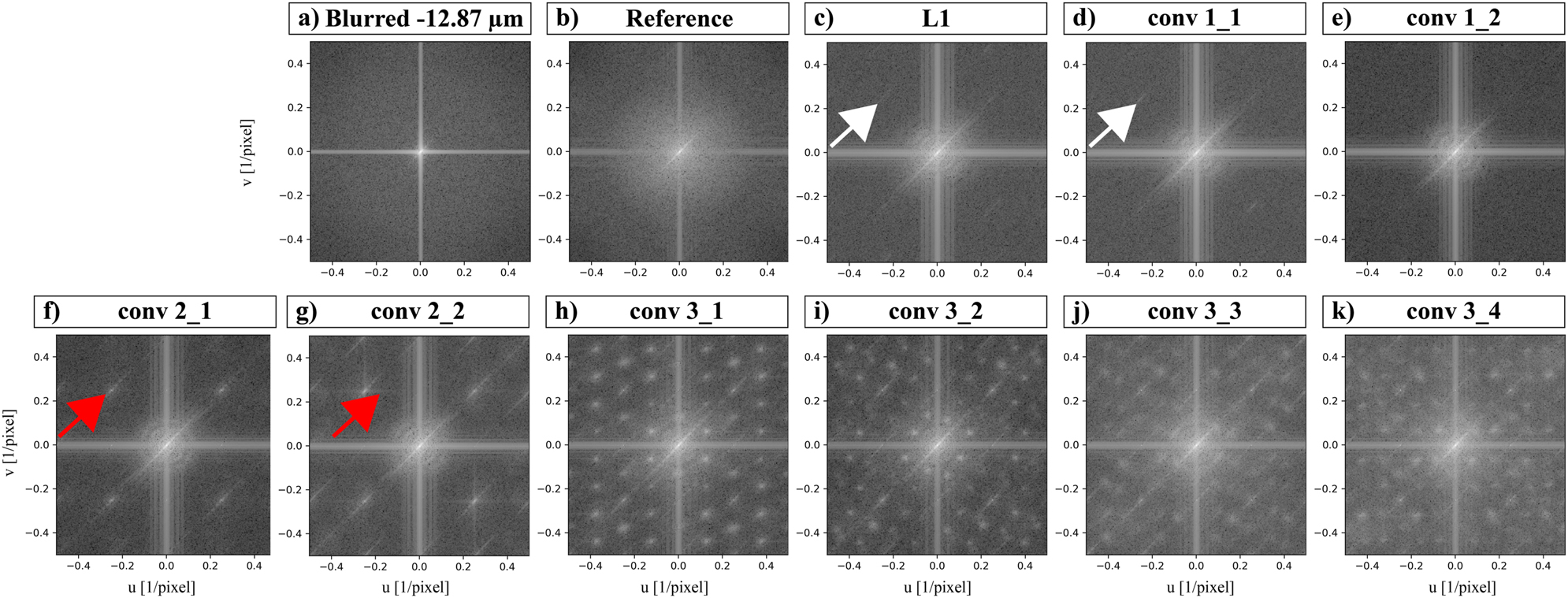
Overview of the perceptual loss results of different feature maps of the VGG-19 model in the frequency domain. The typical pattern for checkerboard artifacts (white arrows) can be observed in the result of the pure L1 loss (c) and the results of the first encoder (d) and (e). This pattern is significantly amplified from the feature maps of the second VGG-19 encoder (f) and (g) (red arrows). The results of the feature maps of the third VGG-19 encoder (h)–(k) show further peaks in the frequency spectrum. For completeness, the blurred (a) and reference (b) acquisitions are displayed in the frequency domain as well.
![Figure 6:
Plot of the horizontal and vertical line profiles across the conspicuities in the frequency spectrum of the feature map conv_2_1. At the frequencies
f
A
=
0.25
1
/
pixel
${f}_{A}=0.25\left[1/\text{pixel}\right]$
and
−
f
A
=
0.25
1
/
pixel
${-}{f}_{A}=0.25\left[1/\text{pixel}\right]$
, distinct peaks with a deviation of 5 dB between the sharp reference image and the restored image can be observed.](/document/doi/10.1515/mim-2024-0012/asset/graphic/j_mim-2024-0012_fig_006.jpg)
Plot of the horizontal and vertical line profiles across the conspicuities in the frequency spectrum of the feature map conv_2_1. At the frequencies
5.2 Experiment 2: are the artifacts dependent on the image quality?
The images presented in Figure 7 are representative of a test series of 30 microscopy images of a lithium-ion battery zoomed in on the graphite anode collected for this experiment. This image series starts with a sharp reference image and then the focus deviation is successively increased with a step size of 0.455 μm. The image row marked in green shows the increasing image blur of the same sample position. It can be observed that fine image details are lost with increasing out-of-focus blur and that objects additionally change in size and shape. For a better comparison, image sections are shown enlarged (colored rectangles). The image row marked in blue shows the restored results of the blurred image row, trained with the feature map conv_2_1 for the perceptual loss. It can be observed that with increasing image blur a more prominent checkerboard pattern occurs. The image row marked in red shows the restored results of the blurred image row, trained with the feature map conv_3_3 for the perceptual loss. Once again, it can be observed that the artifacts become more prominent as the image becomes more blurred.

Light-optical microscopy, brightfield, lithium-ion battery, graphite anode, objective EC Epiplan-Neofluar 20×/0.5 HD DIC M27. Overview of the image deblurring results for increasing image blur. The row marked in green shows the acquired images with an increasing, real out-of-focus blur. The blue row shows the restored images from the deblurring model trained with the feature map conv_2_1 for the perceptual loss. The red row shows the restored images from the deblurring model trained with the feature map conv_3_3 for the perceptual loss. Note that the contrast has been adjusted to improve the visibility of the artifacts for print.
5.3 Experiment 3: can the artifacts be reduced or removed?
First, suitable metrics are determined for the performance evaluation of the image deblurring model to be trained. For this purpose, the dataset created in Experiment 2 is used. Figure 8 shows the course of different metric values for increasing image blur. The x-axis of the partial figures represents the focus deviation in relation to the sharp reference image. The y-axis represents the obtained metric value. A reliable metric must have a linear progression over the increasing focus deviation and thus increasing image blur. For the pixel-based metrics (PSNR, SSIM [35], and MS-SSIM [36]), the MSSSIM shows the best linear graph as the focus deviation increases. The PSNR graph shows an exponential drop at low focus deviations, approaching a linear drop from medium focus deviations. For the SSIM, the graph slowly drops nonlinearly at low focus deviations, approaching a linear drop from medium focus deviations. For the perceptual-based metrics, DISTS [37] shows the best linear graph as the focus deviation increases. The linear slope of LPIPS [38] flattens from the medium focus deviations and becomes saturated at higher ones. The curve of PieApp [39] already reaches its maximum at medium focus deviations before dropping again. Considering the results of Figure 8, the trained models are evaluated using the MS-SSIM and DISTS metrics.

Overview of the courses of the metrics for increasing focus deviation and thus image blur on the image test series. To reliably assess image quality a linear progression over the increasing focus deviation is required. MS-SSIM achieves the best linear progression for pixel-based metrics and DISTS achieves the best for perceptual-based metrics.
Table 2 shows the quantitative evaluation results of the trained models, which were named according to their configuration. Thus, the term VGG conv_2_1 denotes an LVGG loss term with the first feature map of the second encoder, VGG conv_3_3 denotes an LVGG loss term with the third feature map of the third encoder, L f denotes the frequency loss term, and Smooth, Resize, and WT denote the respective architectural modification. According to the perception-distortion trade-off, it can be observed that the use of a ‘pure’ perceptual-loss term leads to an improvement of the DISTS metric and a deterioration of the MS-SSIM (DISTS: 0.162 to 0.143 to 0.113; MS-SSIM: 0.958 to 0.957 to 0.951). The conv_2_1 models achieve further performance improvement with the architecture modifications. The model DHN + L1 + VGG conv_2_1 + WT even achieves an increase of the MS-SSIM to 0.963 compared to the pure L1 loss while at the same time achieving a better DISTS value. The additional use of the frequency loss L f shows an improvement based on the DISTS and a minimal deterioration based on the MS-SSIM. The model DHN + L1 + VGG conv_2_1 + Smooth + L f is an exception, which experiences unstable training due to L f leading to significantly worse performance. Compared to the conv_2_1 models, no clear trend can be observed for the conv_3_3 models. For instance, the Resize modification achieves a minimal improvement in MS-SSIM (0.951–0.952) and a slight deterioration in DISTS (0.113–0.115|0.117). In contrast, the Smooth modification achieves a degradation for both the MS-SSIM (0.951–0.950|0.532), and the DISTS (0.113–0.117|0.467). Furthermore, using the frequency loss L f again leads to unstable model training with the Smooth modification, resulting in the worst performance of all models. The WT modification achieves the best DISTS result while the MS-SSIM score is similar to the pure L1 loss.
Quantitative analysis of the described models on the test dataset. The best results within a model category (conv_2_1, conv_3_3) are shown in bold black. High scores are better for MS-SSIM and lower scores are better for DISTS.
| Model | MS-SSIM ↑ Mean ± Std | DISTS ↓ Mean ± Std |
|---|---|---|
| DHN + L1 | 0.958 ± 0.047 | 0.162 ± 0.079 |
| DHN + L1 + VGG conv_2_1 | 0.957 ± 0.049 | 0.143 ± 0.080 |
| DHN + L1 + VGG conv_2_1 + Resize | 0.959 ± 0.046 | 0.140 ± 0.088 |
| DHN + L1 + VGG conv_2_1 + Resize + L f | 0.955 ± 0.050 | 0.137 ± 0.075 |
| DHN + L1 + VGG conv_2_1 + Smooth | 0.958 ± 0.046 | 0.134 ± 0.083 |
| DHN + L1 + VGG conv_2_1 + Smooth + L f | 0.785 ± 0.100 | 0.339 ± 0.050 |
| DHN + L1 + VGG conv_2_1 + WT | 0.963 ± 0.042 | 0.128 ± 0.083 |
| DHN + L1 + VGG conv_2_1 + WT + L f | 0.960 ± 0.047 | 0.128 ± 0.075 |
| DHN + L1 + VGG conv_3_3 | 0.951 ± 0.053 | 0.113 ± 0.072 |
| DHN + L1 + VGG conv_3_3 + Resize | 0.952 ± 0.052 | 0.115 ± 0.072 |
| DHN + L1 + VGG conv_3_3 + Resize + L f | 0.952 ± 0.052 | 0.117 ± 0.072 |
| DHN + L1 + VGG conv_3_3 + Smooth | 0.950 ± 0.054 | 0.117 ± 0.078 |
| DHN + L1 + VGG conv_3_3 + Smooth + L f | 0.532 ± 0.079 | 0.467 ± 0.023 |
| DHN + L1 + VGG conv_3_3 + WT | 0.957 ± 0.048 | 0.106 ± 0.069 |
| DHN + L1 + VGG conv_3_3 + WT + L f | 0.958 ± 0.046 | 0.106 ± 0.069 |
Figure 9 shows the qualitative evaluation of the trained models on a lithium-ion battery, cathode LiNiCoAlO2 image from the FaMM test dataset. The first row shows an out-of-focus image with an intentional focus deviation of 5.4 μm. For a better comparison of the model performances, the image area marked in green is shown enlarged. The conv_2_1 model results are marked in blue while the conv_3_3 model results are marked in red. Additionally, the result of a pure L1 loss term is shown as a baseline as well as the sharp reference image. Despite improved quantitative results, the Resize, WT, and Smooth architectural modifications for the conv_2_1 models show stronger artifacts compared to the pure conv_2_1 model. The additional optimization using the frequency loss L f clearly reduces the artifacts. Compared to the pure L1 loss, the models w/Resize + L f and w/WT + L f (marked in blue) generate visibly sharper edges. Furthermore, the unstable model training with the combination of Smooth and L f is apparent. For both the conv_2_1 model and the conv_3_3 model, the image content is severely distorted. Compared to the pure conv_3_3 model, the conv_3_3 model with Resize shows reduced artifacts. The edge sharpness is similar to the model conv_2_1 w/Resize + L f . By using the loss term L f (w/Resize + L f ) the image sharpness as well as the artifacts can be improved again. Similar to the conv_2_1 model with WT, the conv_3_3 model with WT continues to generate visible artifacts. Even with the additional optimization using L f , the artifacts can be reduced but remain visible. The architectural modification Smooth achieves a reduction in artifacts but generates blurrier outputs compared to Resize.

Light-optical microscopy, brightfield, lithium-ion battery, cathode LiNiCoAlO2, objective EC Epiplan-Neofluar 20×/0.5 HD DIC M27. A blurred image with an intentional focus deviation of 5.4 μm is used. The results of trained models are shown on an enlarged image region (green) for better comparison. Conv_2_1 model results are marked in blue and conv_3_3 model results are marked in red.
Figure 10 shows a qualitative evaluation of the model results in the frequency domain, with one figure being averaged over all material classes of the entire FaMM test dataset. This provides a better insight into the cause of the artifacts that remain visible in Figure 9. Since the test dataset also contains images with low image blur and checkerboard artifacts become more pronounced with increasing image blur, they are only slightly pronounced in the averaged image of the pure conv_2_1 model (white arrow). In contrast, the ‘blob’ artifacts are still clearly visible for the conv_3_3 model. When using the architectural modification Resize, it can be seen that the magnitudes at the artifact frequency f A are damped, but new peaks (red arrow) are created in the frequency domain. These have a visible effect in the spatial domain as artifacts (Figure 9). The additional use of L f shows that the newly formed peaks are prevented and a homogeneous distribution of the frequencies is achieved. The use of Smooth shows a significant damping of the frequencies around f A (yellow arrow, dark horizontal and vertical lines). The strong damping and thus missing information can be the cause of the visible artifacts. The additional optimization with L f results in an inhomogeneous distribution of the undamped frequencies, which is why the image content is strongly distorted. The use of WT in conv 2 1 models continues to show a significant peak at frequency f A (green arrow) and thus checkerboard artifacts in the image. The additional optimization with L f results in a homogeneous distribution of the frequencies and thus an improvement of the image quality. In contrast, optimization with L f shows no improvement for the conv_3_3 model with WT (pink arrow). The use of Resize on the conv_3_3 model shows a typical pattern for checkerboard artifacts (blue arrow) in addition to the ‘blobs’, which can be corrected by optimizing with L f .

Visualization of the power spectral density (PSD) of individual models averaged over the entire FaMM test dataset.
6 Discussion
Experiment 1 investigated the question of whether the artifacts depend on the feature map used for perceptual loss. The results show that depending on the encoder chosen, there is a tendency to generate some type of artifact. For instance, the feature maps of the second encoder tend to generate checkerboard artifacts, while the feature maps of the third encoder tend to generate ‘blob’ type artifacts. On the other hand, no artifacts are generated with the feature maps of the first encoder. However, the use of the first encoder does not improve the perceptual quality compared to the pure L1 loss. The artifact frequency
Experiment 2 investigated whether the visible artifacts depend on the image quality. The results show that there is a correlation between the level of distortion and artifact generation; higher image blur leads to a more pronounced artifact generation during reconstruction. In Supplementary Materials SM 1, we also show how this is correlated with an increase in the magnitude of the artifact frequency f A as the focus blur increases. Thus, the cost-benefit factor for using perceptual loss depends on the use case. If there is only a small degree of blur in the data, the perceptual loss can be used without concern to increase perceptual quality. As soon as the blur in the data increases or is unknown, further optimizations should be used to reduce the artifacts (see experiment 3). Unfortunately, it cannot be verified at which degree of image blur the artifacts become visible. For a reliable quantitative evaluation, a side-by-side comparison of image quality and the extent of artifacts is required. As far as we know, no metric exists to reliably quantify the presence of the described artifacts, making the thresholds subjective. In Supplementary Materials SM 1, we provide an approach for developing a suitable metric and believe that the research in alternative approaches provides a promising basis for future work. Furthermore, image information such as structures has been shown to have no correlation with the artifacts. One could argue that the stronger the image blur, the higher the information loss, the fewer existing structures in the image, and the more likely the artifacts are generated. However, this argument proves wrong since test images that do not contain any structures except for a few scratches show the same phenomenon – artifacts become prominent as distortion increases.
Experiment 3 investigated whether the artifacts could be reduced or removed using architectural modifications and an additional frequency loss term. First, the results show that not all metrics are suitable for the quantitative evaluation of the trained models on the image deblurring dataset. A reliable metric must have a linear progression over increasing image blur. We advise on testing the metrics for this in advance. Furthermore, a new metric is needed that can quantitatively evaluate the artifacts addressed. The experiment shows that an improvement of DISTS may well show increased artifact generation – even SSIM or MS-SSIM do not offer an alternative in this case. The first two experiments show that checkerboard artifacts are produced when the second encoder is used. Although the architecture modifications Resize, Smooth and WT are supposed to prevent them, this is not the case. Even though the magnitude of the artifact frequency f A can be reduced with Resize and Smooth, Resize introduces new spectral artifacts and Smooth dampens them too heavily, causing valuable information to be lost during model training in order to generate image content. It may be helpful to use pretrained model weights for Smooth to ensure a more stable start to training. WT even increases the magnitude of the artifact frequency f A . Only with the introduction of further optimization with L f , better quantitative and qualitative evaluation results can be achieved. In general, the magnitude of spectral artifacts is reduced, and a homogeneous distribution in the frequency domain is achieved. Furthermore, visibly sharper edges and improved perceptual quality are achieved. An exception is Smooth in combination with L f , which leads to unstable training. Despite better quantitative results of the conv_3_3 models, we recommend using the conv_2_1 models. Based on the qualitative results, it can be observed that the checkerboard artifacts can be reduced more effectively than the ‘blob’ artifacts. In addition, note that the conv_2_1 models, unlike the conv_3_3 models, do not hallucinate and thus do not alter the microstructure. In summary, the model conv_2_1 w/WT + L f achieves the best result. In Supplementary Materials SM 3, we show the transferability of the proposed method using general purpose data and the GOPRO dataset [40]. First, we show that the artifacts become more prominent with increasing motion blur and thus the discussed the phenomenon cannot be limited to focus blur alone. Second, we show that the best model can reduce the artifacts in different domain as well. Our experiments focus primarily on the modifications Resize, Smooth and WT, we provide a brief description of alternative approaches and outline research questions for future work in the Supplementary Materials SM 2.
7 Conclusions
An investigation of the artifacts generated by the perceptual loss term in material microscopy images was conducted in this work. We demonstrated that the feature maps of VGG19’s second encoder show a tendency toward the generation of checkerboard artifacts, while the feature maps of the third encoder show a tendency to ‘blob’ artifacts that make the image look like it was painted on a canvas. Both types of artifacts depend on the level of distortion in the blurred image; the higher the level of blur in the image, the more pronounced the artifacts become. Based on the results from the literature [12], we assume that this is also true for noise. We have shown that commonly used architectural methods to avoid checkerboard artifacts do not help in this case, some even amplifying them. Instead, we achieve further optimization by introducing a frequency loss term, which helps to achieve quantitatively and qualitatively better results. We recommend replacing the down- and upsampling layers in a model with the wavelet transform layers proposed by Ref. [29] and adding the introduced frequency loss term to the loss function when using a perceptual loss term in a ratio of 1,000:1 of α to β. In material microscopy, the proposed method offers the advantage of reconstructing blurred images more accurately, thus ensuring a reliable quantitative microstructure analysis. Especially methods for image deblurring, which are applied to already recorded image data or in situ during data acquisition at the microscope, can benefit from the proposed method. Furthermore, in Supplementary Materials SM 3, we demonstrate the transferability of the proposed method on general purpose data and show that the our method can reduce the artifacts.
We have also shown that not all common metrics in the field of image deblurring show a linear progression with increasing blur. We recommend investigating which metric to use for a given dataset prior to model training. Furthermore, a new metric is needed that is sensitive to the artifacts addressed generated by the perceptual loss term.
Funding source: Bundesministerium für Bildung und Forschung
Award Identifier / Grant number: 13FH176PX8
Funding source: Aalen University of Applied Sciences
-
Research ethics: Not applicable.
-
Informed consent:Not applicable.
-
Author contributions: The authors have accepted responsibility for the entire content of this manuscript and approved its submission.
-
Use of Large Language Models, AI and Machine Learning Tools: None declared.
-
Conflict of interests: The authors state no conflict of interest.
-
Research funding: Publication funded by Aalen University of Applied Sciences as well as by the Federal Ministry of Education and Research of Germany provided for the EBiMA project (13FH176PX8) funded in the FHprofUnt program.
-
Data availability: The datasets analysed during the current study are available on IEEE Dataport at https://doi.org/10.21227/vwrx-yw83.
References
[1] H. Zhao, O. Gallo, I. Frosio, and J. Kautz, “Loss functions for image restoration with neural networks,” IEEE Trans. Comput. Imag., vol. 3, no. 1, pp. 47–57, 2017. https://doi.org/10.1109/tci.2016.2644865.Search in Google Scholar
[2] A. Mustafa, et al.., “Training a task-specific image reconstruction loss,” in 2022 IEEE/CVF Winter Conference on Applications of Computer Vision (WACV), 2022, pp. 21–30.10.1109/WACV51458.2022.00010Search in Google Scholar
[3] A. Abdelhamed and M. Afifi, “Ntire 2020 challenge on real image denoising: dataset, methods and results,” in 2020 IEEE/CVF Conference on Computer Vision and Pattern Recognition Workshops (CVPRW), 2020, pp. 2077–2088.Search in Google Scholar
[4] Y. Blau and T. Michaeli, “The perception-distortion tradeoff,” in 2018 IEEE/CVF Conference on Computer Vision and Pattern Recognition, 2018, pp. 6228–6237.10.1109/CVPR.2018.00652Search in Google Scholar
[5] Z. Wang and A. C. Bovik, “Mean squared error: love it or leave it? A new look at signal fidelity measures,” IEEE Signal Process. Mag., vol. 26, no. 1, pp. 98–117, 2009. https://doi.org/10.1109/msp.2008.930649.Search in Google Scholar
[6] Y. Blau and T. Michaeli, “Rethinking lossy compression: the ratedistortion-perception tradeoff,” in Proceedings of the 36th International Conference on Machine Learning, ICML 2019, 9–15 June, vol. 97, Long Beach, California, USA, PMLR, 2019, pp. 675–685.Search in Google Scholar
[7] Z. Fu, et al., “Edge-aware deep image deblurring,” Neurocomputing, vol. 502, pp. 37–47, 2019.10.1016/j.neucom.2022.06.051Search in Google Scholar
[8] O. Kupyn, et al.., “Deblurgan: blind motion deblurring using conditional adversarial networks,” in 2018 IEEE/CVF Conference on Computer Vision and Pattern Recognition, 2018, pp. 8183–8192.10.1109/CVPR.2018.00854Search in Google Scholar
[9] O. Kupyn, et al.., “Deblurgan-v2: deblurring (orders-of-magnitude) faster and better,” in 2019 IEEE/CVF International Conference on Computer Vision (ICCV), 2019, pp. 8877–8886.10.1109/ICCV.2019.00897Search in Google Scholar
[10] S. Nah, et al.., “Clean images are hard to reblur: exploiting the ill-posed inverse task for dynamic scene deblurring,” 2022, arXiv:2104.12665.Search in Google Scholar
[11] Y. Wen, et al., “Structure-aware motion deblurring using multi-adversarial optimized cyclegan,” IEEE Transactions on Image Processing, vol. 30, no. 1, pp. 6142–6155, 2021. https://doi.org/10.1109/tip.2021.3092814.Search in Google Scholar
[12] M. Deng, A. Goy, S. Li, K. Arthur, and G. Barbastathis, “Probing shallower: perceptual loss trained phase extraction neural network (plt-phenn) for artifact-free reconstruction at low photon budget,” Opt. Express, vol. 28, no. 2, pp. 2511–2535, 2020. https://doi.org/10.1364/oe.381301.Search in Google Scholar PubMed
[13] Q. Yang, et al.., “Low-dose ct image denoising using a generative adversarial network with wasserstein distance and perceptual loss,” IEEE Trans. Med. Imag., vol. 37, no. 6, pp. 1348–1357, 2018. https://doi.org/10.1109/tmi.2018.2827462.Search in Google Scholar
[14] J. Johnson, A. Alahi, and L. Fei-Fei, “Perceptual losses for real-time style transfer and super-resolution,” in Computer Vision – ECCV 2016, B. Leibe, J. Matas, N. Sebe, and M. Welling, Eds., Cham, Springer International Publishing, 2016, pp. 694–711.10.1007/978-3-319-46475-6_43Search in Google Scholar
[15] P. Krawczyk, A. Jansche, T. Bernthaler, and G. Schneider, “Increasing the image sharpness of light microscope images using deep learning,” Pract. Metallogr., vol. 58, no. 11, pp. 684–696, 2021. https://doi.org/10.1515/pm-2021-0061.Search in Google Scholar
[16] Y. Bai, Y. Guo, J. Wei, L. Lu, R. Wang, and Y. Wang, “Fake generated painting detection via frequency analysis,” in 2020 IEEE International Conference on Image Processing (ICIP), 2020, pp. 1256–1260.10.1109/ICIP40778.2020.9190892Search in Google Scholar
[17] A. Odena, V. Dumoulin, and C. Olah, “Deconvolution and checkerboard artifacts,” Distill, 2016. Available at: http://distill.pub/2016/deconv-checkerboard [Accessed: Jul. 16, 2024.]10.23915/distill.00003Search in Google Scholar
[18] F. Juefei-Xu, R. Wang, and Y. Huang, “Countering malicious deepfakes: survey, battleground, and horizon,” Int. J. Comput. Vis., vol. 130, no. 7, pp. 1678–1734, 2022. https://doi.org/10.1007/s11263-022-01606-8.Search in Google Scholar PubMed PubMed Central
[19] M. Barni, et al.., “Cnn detection of gangenerated face images based on cross-band co-occurrences analysis,” in 2020 IEEE International Workshop on Information Forensics and Security (WIFS), 2020, pp. 1–6.10.1109/WIFS49906.2020.9360905Search in Google Scholar
[20] J. Frank, et al.. “Leveraging frequency analysis for deep fake image recognition,” in Proceedings of the 37th International Conference on Machine Learning, ser. Proceedings of Machine Learning Research, H. DaumeIII and A. Singh, Eds., vol. 119. PMLR, 2020, pp. 3247–3258.Search in Google Scholar
[21] Y. Yao, et al.., “Attention-aware multi-stroke style transfer,” in 2019 IEEE/CVF Conference on Computer Vision and Pattern Recognition (CVPR), 2019, pp. 1467–1475.10.1109/CVPR.2019.00156Search in Google Scholar
[22] J.-Y. Zhu, et al.., “Unpaired image-to-image translation using cycle-consistent adversarial networks,” in 2017 IEEE International Conference on Computer Vision (ICCV), 2017, pp. 2242–2251.10.1109/ICCV.2017.244Search in Google Scholar
[23] X. Chen, et al.., “Gated-gan: adversarial gated networks for multi-collection style transfer,” IEEE Trans. Image Process., vol. 28, no. 2, pp. 546–560, 2019. https://doi.org/10.1109/tip.2018.2869695.Search in Google Scholar PubMed
[24] Y. Huang, et al.., “Fakepolisher: making deepfakes more detection-evasive by shallow reconstruction,” in Proceedings of the 28th ACM International Conference on Multimedia, ser. MM ’20, New York, NY, USA, Association for Computing Machinery, 2020, pp. 1217–1226.10.1145/3394171.3413732Search in Google Scholar
[25] C. Dong, A. Kumar, and E. Liu, “Think twice before detecting gangenerated fake images from their spectral domain imprints,” in 2022 IEEE/CVF Conference on Computer Vision and Pattern Recognition (CVPR), 2022, pp. 7855–7864.10.1109/CVPR52688.2022.00771Search in Google Scholar
[26] Y. Sugawara, S. Shiota, and H. Kiya, “Checkerboard artifacts free convolutional neural networks,” APSIPA Trans. Signal Inf. Process., vol. 8, no. 1, 2019, https://doi.org/10.1017/ATSIP.2019.2.Search in Google Scholar
[27] W. Shi, et al.., “Real-time single image and video superresolution using an efficient sub-pixel convolutional neural network,” in 2016 IEEE Conference on Computer Vision and Pattern Recognition (CVPR), 2016, pp. 1874–1883.10.1109/CVPR.2016.207Search in Google Scholar
[28] Y. Kinoshita and H. Kiya, “Fixed smooth convolutional layer for avoiding checkerboard artifacts in cnns,” in ICASSP 2020 – 2020 IEEE International Conference on Acoustics, Speech and Signal Processing (ICASSP), 2020, pp. 3712–3716.10.1109/ICASSP40776.2020.9054096Search in Google Scholar
[29] P. Liu, et al.., “Multi-level wavelet-cnn for image restoration,” in 2018 IEEE/CVF Conference on Computer Vision and Pattern Recognition Workshops (CVPRW), 2018, pp. 886–88609.10.1109/CVPRW.2018.00121Search in Google Scholar
[30] H. Zhang, et al.., “Deep stacked hierarchical multi-patch network for image deblurring,” in 2019 IEEE/CVF Conference on Computer Vision and Pattern Recognition (CVPR), 2019, pp. 5971–5979.10.1109/CVPR.2019.00613Search in Google Scholar
[31] P. Krawczyk, et al.., “Comparison of deep learning methods for image deblurring on light optical materials microscopy data,” in 2021 IEEE 17th International Conference on Automation Science and Engineering (CASE), 2021, pp. 1332–1337.10.1109/CASE49439.2021.9551404Search in Google Scholar
[32] Y. Bengio and Y. LeCun, Eds. 3rd International Conference on Learning Representations, ICLR 2015, San Diego, CA, USA, May 7–9, 2015, Conference Track Proceedings, 2015.Search in Google Scholar
[33] J. Deng, et al.., “Imagenet: a large-scale hierarchical image database,” in 2009 IEEE Conference on Computer Vision and Pattern Recognition, 2009, pp. 248–255.10.1109/CVPR.2009.5206848Search in Google Scholar
[34] P. Krawczyk, et al., “Focus and motion blur in microscopy (FaMM),” IEEE Dataport, 2023. https://doi.org/10.21227/vwrx-yw83.Search in Google Scholar
[35] Z. Wang, et al.., “Image quality assessment: from error visibility to structural similarity,” IEEE Trans. Image Process., vol. 13, no. 4, pp. 600–612, 2004. https://doi.org/10.1109/tip.2003.819861.Search in Google Scholar PubMed
[36] Z. Wang, E. Simoncelli, and A. Bovik, “Multiscale structural similarity for image quality assessment,” in The Thrity-Seventh Asilomar Conference on Signals, Systems and Computers, vol. 2, 2003, pp. 1398–1402.Search in Google Scholar
[37] K. Ding, et al.., “Image quality assessment: unifying structure and texture similarity,” IEEE Trans. Pattern Anal. Mach. Intell., vol. 44, no. 5, pp. 2567–2581, 2022. https://doi.org/10.1109/TPAMI.2020.3045810.Search in Google Scholar PubMed
[38] R. Zhang, et al.., “The unreasonable effectiveness of deep features as a perceptual metric,” in 2018 IEEE/CVF Conference on Computer Vision and Pattern Recognition, 2018, pp. 586–595.10.1109/CVPR.2018.00068Search in Google Scholar
[39] E. Prashnani, et al.., “Pieapp: perceptual imageerror assessment through pairwise preference,” in 2018 IEEE/CVF Conference on Computer Vision and Pattern Recognition, 2018, pp. 1808–1817.10.1109/CVPR.2018.00194Search in Google Scholar
[40] S. Nah, T. H. Kim, and K. M. Lee, “Deep multi-scale convolutional neural network for dynamic scene deblurring,” in 2017 IEEE Conference on Computer Vision and Pattern Recognition (CVPR), 2017, pp. 257–265.10.1109/CVPR.2017.35Search in Google Scholar
Supplementary Material
This article contains supplementary material (https://doi.org/10.1515/mim-2024-0012).
© 2024 the author(s), published by De Gruyter on behalf of Thoss Media
This work is licensed under the Creative Commons Attribution 4.0 International License.
Articles in the same Issue
- Frontmatter
- Editorial
- What is open access and what is it good for?
- News
- Community news
- View
- Optical sectioning in fluorescence microscopies is essential for volumetric measurements
- Review Article
- Wrapped up: advancements in volume electron microscopy and application in myelin research
- Research Articles
- Reducing artifact generation when using perceptual loss for image deblurring of microscopy data for microstructure analysis
- Utilizing collagen-coated hydrogels with defined stiffness as calibration standards for AFM experiments on soft biological materials: the case of lung cells and tissue
- Phase characterisation in minerals and metals using an SEM-EDS based automated mineralogy system
- Corrigendum
- Corrigendum to: FAST-EM array tomography: a workflow for multibeam volume electron microscopy