Possible impact of construction activities around a permanent GNSS station – A time series analysis

3.1 Analysis in the observation domain

Both code and carrier phase observations can be interpreted as pseudorange observations between a satellite at the time of signal emission and a receiver at the time of signal reception (Hofmann-Wellenhof and Wasle 2008).

Denoting code observation with P and carrier phase observation with ϕ , simplified models for the observations are given by:

where ρ is the geometric distance between a satellite at the time of signal emission and a receiver at the time of signal reception, c is the speed of light, d t and d T are the receiver and satellite clock errors, respectively, I i is the ionospheric delay, T is the tropospheric delay, M P i and M ϕ i are the multipath effects on code and carrier phase, respectively, N i is the carrier phase ambiguity, and λ i is the wavelength of the carrier phase signal. Index i is used to assign the frequency of the carrier phase signal. For example, for GPS, i = 1 or i = 2 implies the use of f 1 = 1575.42 MHz or f 2 = 1227.60 MHz. Most GNSS systems transmit signals at more than two different frequencies; i = 1 , 2 , 3 , … .

Since terms like relativistic effects, code and carrier phase hardware delays in satellite and receiver are not relevant for our approach to quantification of quality numbers, they are omitted in equations (1) and (2). However, it must be mentioned that carrier phase observations are much more precise than code observations, by approximately two orders of magnitude.

We notice the inclusion of N i λ i in equation (2) to account for the ambiguity of the carrier phase observable and that the ionospheric term has an opposite sign for code and carrier phase.

The first-order ionospheric delay at frequency f i is given by Hofmann-Wellenhof and Wasle (2008):

where TEC (total electron content) is the integral of the electron density along the ray path between the satellite and receiver. TEC provides the number of electrons per square meter and is usually given in units where one TEC unit is 1 0 16 m − 2 . As seen in equation (3), the ionospheric delay is inversely proportional to the square of the carrier frequency. Hence, the ionospheric delay at frequency f j can be expressed as a function of the delay at another frequency f i :

Frequency index j represents any frequency that is different from i . It is now readily seen that the ionospheric delay can be estimated from dual-frequency observations. Subtracting carrier phase observations given by equation (2) using f i and f j frequencies, we obtain:

We now adopt the approach used by Estey and Meertens (1999). The starting point is the knowledge that carrier phase observations are two orders of magnitude more precise than code observations. Similarly, multipath on carrier phase observations is considered negligible compared to multipath on code observations. Subtracting phase observations from code observations on frequency f i gives

Inserting the ionospheric delay, I i , from equation (5) and rearranging gives the estimated code multipath on the f i frequency:

B i is a bias term due to carrier phase ambiguities and M P ϕ i is due to multipath on carrier phase observations;

In the following, the carrier phase multipath term M P ϕ i is considered small enough to be neglected. The bias term, B i , remains constant as long as there are no cycle slips in the carrier phase observations.

To identify eventual cycle slips, we monitor the continuity in the time-series of ionospheric delays computed using equation (5). Sudden jumps in ionospheric delay from epoch to epoch that cannot be explained by ionospheric time-variation are used as indicators of cycle slips, see Hofmann-Wellenhof and Wasle (2008) and Estey and Meertens (1999). For each satellite and continuous arc of carrier phase observations, a , we estimate average bias terms:

where k is the epoch number and n a is the number of epochs in arc a . Each cycle slip will introduce a new arc, a , with an associated bias term. Standard deviations s M P i for each satellite are computed as the square root of the weighted sum of all squared differences between average bias terms and epoch-wise code multipath divided by the total number of epochs minus the number of arcs.

In equation (11), n tot is the total number of epochs used in the computations, n arc is the number of continuous arcs, and w k is an elevation angle-dependent weight for observations at epoch k . We have used the following weighting function:

where β is the satellite’s elevation angle, Roald (2020).

GNSS Receiver QC 2020

The in-house Matlab software “GNSS Receiver QC 2020” routine was used for the analysis in the observation domain, Roald (2020). This software takes observation files in the RINEX 3 format and satellite coordinates in SP3 format as input and estimates the code multipath numbers using the approach outlined earlier. It applies both a geometry free and a semi-geometry-dependent approach.

The result files were imported into Python for additional analysis and presentation. The focus of interest lies in the standard deviations of multipath, particularly the weighted estimates that incorporate the elevation angle of the satellites. Standard deviations are computed as average values across all satellites. In addition, information about the number of observations and estimates per signal, cycle slips, and the average elevation angle were also extracted for each combination (Roald 2020). To ensure a consistent data set, a simplified standard deviation based outlier detection approach was used (Ghilani 2018, chapter three, pp. 39–55).

These calculations are quite time-consuming. An important factor that increases processing time is that Matlab, by default, cannot fully utilize all the computer’s processor cores. Only a few cores will be “activated.” To enhance processing efficiency, a Python script was developed that utilizes multiprocessing to execute a Matlab function responsible for data retrieval and running the routine. This approach allows simultaneous analysis of multiple years and maximizes the utilization of the computer’s processing capacity (Aarnes 2022, p. 72–75). To create polar plots, check the signal-to-noise ratio (SNR), and study estimates on individual satellites, the in-house software “GNSS Multipath Analysis Software” was used (Aarnes 2022).

3.2 Analysis in the coordinate domain

The analysis in the coordinate domain includes:

• Precise point positioning (PPP)

• Relative GNSS positioning.

Relative GNSS positioning utilizes simultaneous observations from multiple receivers so that common errors between the stations get eliminated or at least get heavily reduced. The extent to which the errors are reduced, largely depends on the distance between the stations.

For this analysis, the RTKLIB library was utilized, (Takasu 2013). RTKLIB is an open source software package designed for real-time and postprocessing of GNSS data. It is primarily used for positioning applications, including real-time kinematic (RTK) positioning, PPP, and other related GNSS data processing tasks. In this study, mainly the command-line program RNX2RTKP was used. However, this application had a bug in the SP3 file reader routine (RTKLIB 2.4.3 b34). If the number of satellites in the SP3 file exceeded 99, just a few satellites were read in. The bug has number 152 on RTKLIB’s support website’s list of known issues (Takasu 2021). To fix this, a change had to be made to line 91 of the source code of the “preceph.c” function. To implement the code changes, RTKPOST and RNX2RTKP had to be recompiled into a new executable file.

To automate the calculation processes in RTKLIB, two Python scripts were developed: one for the PPP solution and one for the relative solution. The scripts have a similar structure and retrieve necessary data from different locations on the hard drive, copying them to a common working directory.

A Python script was developed for further analysis of the results in RTKLIB’s pos format. The script performs a simple outlier detection, calculates annual averages, root mean square error (RMSE), and other relevant statistics. The outlier detection procedure is similar to the one used in the observation domain. The results are stored in various plots and tables in text format. For the PPP solution, a geodetic transformation of the station coordinates for each daily solution was also carried out. The station coordinates were transformed from the dynamic reference frame ITRF14 at the current epoch to the static reference frame ETRS89. In the same way as in the observation domain, linear trend lines were calculated based on the average RMSE from the PPP and baseline calculations.

3.3 Cross-validation

To cross-validate the results against an independent source, InSAR was chosen due to its ability to capture small changes over time with high temporal resolution. The Norwegian Geological Survey (NGU) operates a web service called “InSAR Norge” that provides radar data dating back to 2008 (NGU 2023). The estimates were based on an average of several points defined by a polygon. The analysis was conducted using the “Radarsat-2” (Descending, Oslofjord area) and “Sentinel-1” (Descending 2) datasets.

3.4 Covariance matrix reconstruction and error propagation

The output coordinate system in RTKLIB was set to ECEF (Earth centred Earth fixed), meaning that the estimated standard deviations are given for geocentric coordinates. To transform the standard deviations from ECEF to a local topocentric coordinate system, the general law of propagation was utilized. Based on the output from RKTLIB, it is possible to fully reconstruct the variance–covariance matrix. In the result file (.pos), this information is given as sdx, sdy, sdz, sdxy, sdyz, and sdzx. The first three values represent the estimated standard deviation for X-, Y-, and Z-coordinates. These values are squared and placed along the diagonal of the covariance matrix. The other three values are related to the co-variances. According to RTKLIB’s manual, the absolute value of sdxy, sdyz, and sdzx equals the square root of the absolute value of the covariances XY, YZ, and ZX, respectively, and the sign represents the sign of the covariance. Thus, these parameters must also be squared to obtain the covariance, but it is mandatory to maintain the sign. Using the numpy-sign syntax (NumPy 2024), the full covariance matrix Σ is given by

The covariance matrix in the local topocentric ENU-system (East, North, Up) is determined by using the general law of error propagation (Ghilani 2018):

where M is the rotation matrix that transforms coordinates from ECEF to ENU and is given by:

where φ and λ are the latitude and longitude of the receiver, respectively. The standard deviation of the east, north, and up components are then given by the square root of the diagonal elements of Σ ′ .

5.1 Relative GNSS

The most important settings for the relative GNSS solution are shown in Table 4. Both the rover and base station antenna types were added, along with the base station coordinates. Default RTKLIB settings were used for all other parameters. It is worth noting that a carrier phase float solution was selected instead of a carrier phase integer solution (FIX) due to RTKLIB having difficulties obtaining consistent FIX solutions when utilizing the ionospheric-free linear combination.

5.2 PPP

The most important settings for PPP are shown in Table 5.

Correction files for Earth rotation parameters (ERPs) and DCBs were added by generating a new configuration file with updated paths for each day in the time series. The reason for doing this is that in RTKLIB these correction files cannot be specified as arguments. Furthermore, the antenna correction file (IGS14.atx) and the correction file for ocean tide loading were also added to the configuration file.

To minimize the influence of the troposphere, both the delay in zenith and the gradient parameters were estimated as additional parameters. Furthermore, the a priori standard deviation of the phase observations was adjusted from the default value of 0.003 to 0.010 m. In addition, the ratio between code and phase measurements was increased from 100 to 300. The a priori standard deviation for the GLONASS phase observations was adjusted to 0.050 m so that not too many epochs would be selected as outliers. These adjustments are based on extensive testing with different values, and the configuration shown in Figure 5 is the one that produced the best results in this case.

5.3 Observation domain

The average elevation angle and the number of observations are plotted as a function of time and are presented in Figure 2. It is important to note that the number of operational Galileo satellites was significantly lower than other systems when the receiver was replaced in January 2015. The increase in the number of observations is shown in Figure 2 and does not level off until the end of 2019. Other interesting observations are that the number of C2X observations for GPS varies in the period before the receiver is replaced, and there is a jump in the number of C2X observations for BeiDou in 2019. This is because the receiver did not start logging BeiDou-3 and the C6X signal until the end of January 2019, which coincides with a firmware update. When it comes to the multipath estimates, there is a clear increasing trend for the C1C signal for GPS and GLONASS. This increase started in 2015. Multipath plotted as a function of time is shown for the C1C signal for both GPS and GLONASS in Figure 3.

Figure 2

The average elevation angle and number of observations for each signal and system (per day).

Figure 3

Multipath effects over time for the C1C signal (GPS & GLONASS).

The annual mean of the weighted standard deviations and the respective trend lines are presented in Figure 4.

Figure 4

Annual standard deviations of multipath with first-order trend lines.

Similar scaling on the y -axis makes the increase less apparent, a plot showing only C1C for GPS and GLONASS is presented in Figure 5.

Figure 5

Annual standard deviation values for multipath estimates of the C1C signal.

The SNR for each signal and system is shown as annual averages in Figure 6.

Figure 6

Annual averages of SNR for each signal and system.

Note the high SNR for C8X (Galileo E5 AltBOC). A polar plot was created for each day to see where the effect of multipath is greatest relative to the receiver. Interestingly, the Munch museum building is blocking the lower parts of the satellite orbit in the southeast direction. See Figure 7.

Figure 7

Polarplot of multipath. The Munch Museum building is apparently blocking parts of the satellite orbit. Shown with the green box. Left plot: 8 July 2016. Right plot: 25 December 2017.

5.4 Relative GNSS results

For GPS and GLONASS, there is an increasing trend in RMSE for the eastern component (Figure 8).

Figure 8

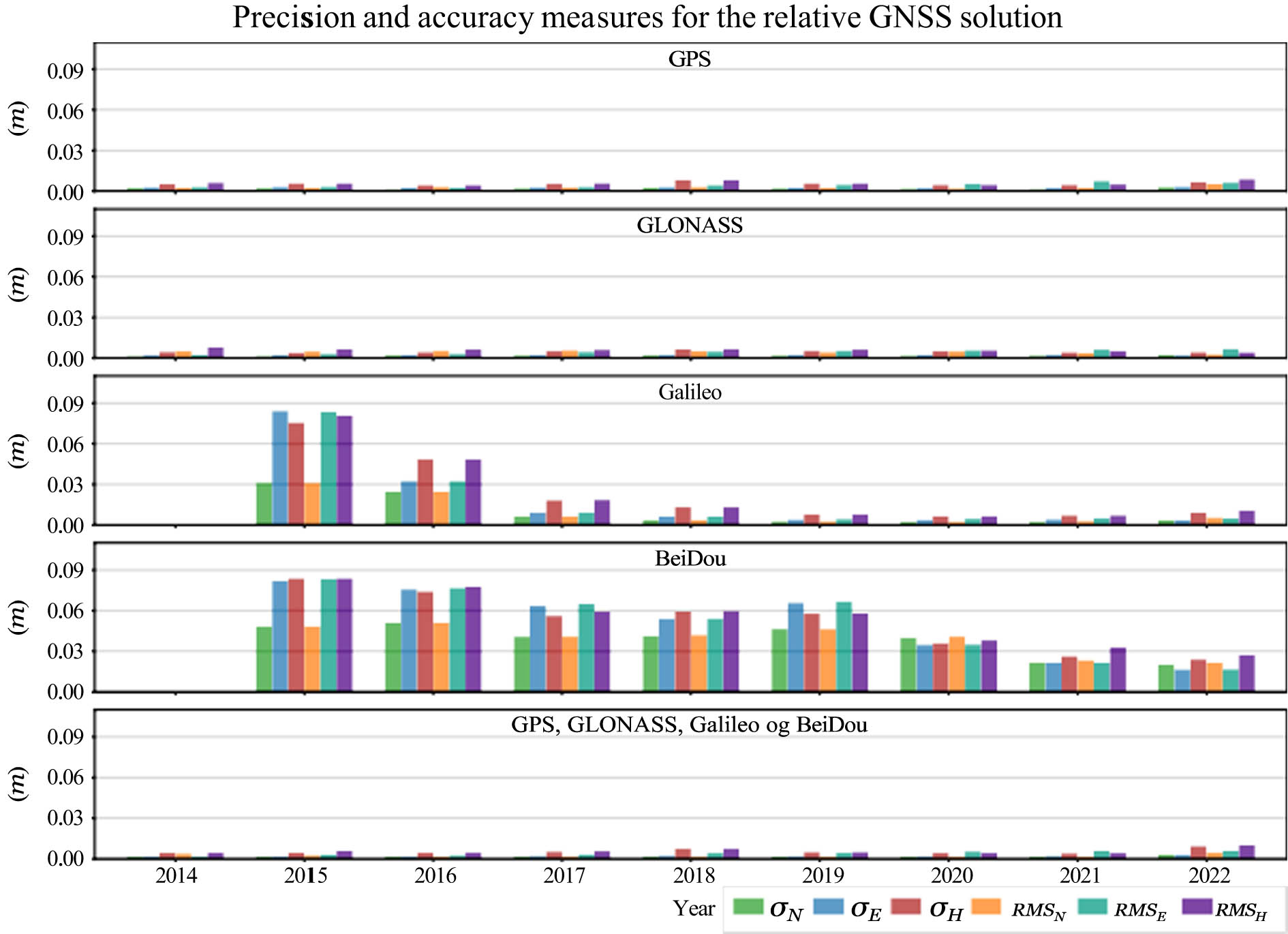
Bar plot showing standard deviation and RMSE for the relative GNSS solution.

Due to the big differences in the statistical values in Figure 8, the values for GPS, GLONASS, and multi-GNSS are presented in Figure 9 with a different y-axis scaling.

Figure 9

Bar plot showing standard deviation and RMSE for the relative GNSS solution.

In Figure 10, annual RMSE and trendlines are plotted. The increasing trend in the eastern component is clear for the GPS, GLONASS, and multi-GNSS solution. Note that it is essential to consider the r 2 number when looking at trends, which is high, especially for GLONASS, which shows that a linear model fits the annual RMSE well.

Figure 10

Annual RMSE with first-order trend lines for GPS, GLONASS, and multi-GNSS (relative GNSS).

5.5 PPP results

The results from the PPP solution are presented in form of plots. Standard deviation and RMSE are shown in Figure 11.

Figure 11

Bar plot showing standard deviation and RMSE for the PPP solution.

As a consequence of large differences in accuracy between the systems, an equal scaling makes it difficult to see the actual level of accuracy for some of the solutions. Diagrams with a different scaling are shown in Figure 12.

Figure 12

Bar plot showing standard deviation and RMSE for the PPP solution.

As Figure 12 shows, the accuracy increases from the beginning to the end of the time series, i.e., the RMSE become smaller. Note the high RMSE for GLONASS in the period between 2010 and 2015.

5.6 Cross-validation

Based on the results from “InSAR Norge,” the average motion velocity was calculated to be − 0.12  mm/a and − 0.60  mm/a for Radar-2 and Sentinel-1, respectively. The calculated displacement is presented in Figure 13.

5.7 Artefacts

In 2019, something notable happened with the multipath estimates for Galileo. A sudden increase in standard deviations for both weighted and non-weighted estimates happened and for all signals simultaneously. This is shown in Figure 14.

Figure 13

The estimated displacement based on the points within the polygon.

Since the high standard deviations occur on all signals simultaneously, it is natural to suspect bugs in the receiver software. If the increase in standard deviations is associated with the software update log, the timing exactly coincides with an update. As shown in Table 3, the receiver was updated on January 31, 2019. This software remained installed until a new update on September 16, 2019. These two dates correspond to DOY (day of year) 31 and 259, which coincide entirely with the shaded area in Figure 14. Therefore, it can be claimed with reasonable certainty that these jumps are software-related and thus do not represent an actual increase in multipath.

6.1 Observation domain

It is expected that various signals are affected differently by multipath. This is due to several factors, but the main differences can be broken down into three signal properties: the chip rate of the signal, signal strength, and modulation technique. These expectations are confirmed by comparing the results from various signal combinations.

An important remark when comparing the statistical values is to be aware that the data basis for the different signals is different. For example, the number of observations for C1C and C2W for GPS is relatively constant throughout the time series. This is not the case for C2X and C5X, which have an increase in number of observations as the satellite constellation changes. Therefore, signals that have had a stable number of observations are better suited to determine the extent to which construction activities have led to a change in multipath.

The results of the analysis in the observation domain reveal a significant increase in standard deviations for the C1C signal for both GPS and GLONASS. The estimates are calculated based on a robust data set throughout the time series, and the variation from year to year is small. This is clearly illustrated in Figure 4. The regression model also fits well with the data points for these signals. In addition, the polar plots exhibit the same trend, as depicted in the snapshot in Figure 7. The level of multipath seems more pronounced in 2017 compared to 2016, a pattern observed beyond just this single snapshot. At first glance, it might seem strange that the highest multipath values are in the southwest direction, given that there are no obstructions in that direction and all the new buildings are in the north east direction. However, in a polar plot, the dots represent the positions of satellites relative to the receiver. Consequently, the reflected signal may originate from the opposite direction from what’s shown in the plot. In Figure 15, the new buildings are visualized.

Figure 14

The shaded area shows the period with high standard deviations for Galileo.

All these factors suggest that the increase is indeed real. Another interesting observation from this plot is that the signals appear to have a common increase in standard deviations between 2015 and 2018. Comparing aerial photographs shows that the most significant changes occurred precisely during this period. See Figure 16. As mentioned earlier, a high chip rate makes the signal more robust against multipath. Therefore, it is unsurprising that the results show an increase for the C1C signal of GPS and GLONASS, which have rates of 1.023 and 0.511 Mcps, respectively. This means that one chip is approximately 300 and 600 m, respectively. Both Deichman, Munch Museum, and large parts of the row of high-rise buildings known as “Barcode,” are within a range of 300 m from the antenna. The fact that the buildings are within one chip length means that they can cause an increased occurrence of reflected signals.

Figure 15

Image exported from Google Earth that shows the buildings in the north-east direction of the receiver.

The reason why there is no increase for signals with higher chip rates may be due to the fact that the distance to new buildings simply becomes too large.

Considering that C2W has a 10 times higher chip rate than C1C, it is somewhat surprising that the standard deviations for C2W are higher for much of the time series. One possible explanation is that C2W is actually a signal consisting of an encrypted code that is not publicly available. However, many geodetic receivers can derive code and phase measurements without knowing the encrypted code. The unknown code is then estimated using various techniques, such as “Z-tracking.” Such methods, however, are not entirely problem free, and the quality of the constructed signal is not equivalent to the “real signal.” It leads to a considerable increase in noise, and since the multipath estimates include measurement noise, it may be the cause.

The AltBOC modulation leads to more narrow and distinct correlation peaks. This helps the receiver to distinguish a direct signal from a reflected signal that arrives with a slight delay. A signal that uses this technique is the Galileo E5 AltBOC signal. In the RINEX format, this signal has the code C8X. In addition to a more advanced modulation technique, Galileo E5 AltBOC also has a high chip rate (10.23 Mcps) and high signal strength. Hence, in theory, the C8X signal is more robust against multipath than other signals. The analysis results in the observation domain show that this is also true in practice. C8X has considerably lower standard deviations than other signals, which is in accordance with findings in other studies, e.g., Simsky et al. (2023) and Zaminpardaz and Teunissen (2017). Based on the annual average of standard deviations, C1X has almost twice as high values as C8X. It also has a much higher SNR than other signals. See Figure 6. In summary, C8X is the signal that performs by far the best of all the signals analyzed in this study. This shows that the signal is better able to compensate for local influences.

Galileo and BeiDou had only a few operational satellites when the receiver was replaced in 2015. Estimates on single satellites were also studied to remove the influence of the satellite constellation expansion. However, it was not proven that the construction activity has led to a significant increase in multipath for either of the signals.

6.2 Relative GNSS

The relative GNSS solution performed well throughout the entire time series and provides a good basis for examining changes in accuracy. Results from GPS, GLONASS, and multi-GNSS solutions show a rising trend for the east component, as shown in Figure 8. The trend plot in Figure 10 also shows a slight trend in the height component, but since the RMSE are quite scattered and r 2 is very low, this is likely random variation.

For GLONASS and the multi-GNSS solution, the trend in the east component is more apparent than for GPS. The average RMSE are closer to the regression lines, and r 2 is over 0.95 for both solutions compared to 0.81 for GPS. A common feature for GPS, GLONASS, and the multi-GNSS solutions is that the RMSE for the eastern component started increasing around 2017. Since most of the construction activity took place during this period, and an increase in the observation domain can also be seen at the same time, there are several indications that the construction activity has had an impact on position accuracy. The RMSE for the east component has increased from around 2 to 3 mm to approximately 6 mm for GPS, GLONASS, and multi-GNSS solutions. This is a significant increase in percentage terms, but the uncertainty in the position estimates must also be considered. There will be some random variation, but at least part of the increase is likely due to the increased effect of multipath interference.

A somewhat surprising result was that the accuracy in the east component was lower than that in the north component for most of the time series. Due to the lower number of satellites in the northern direction in Norway, satellite geometry typically leads to the opposite result. Figure 8 shows that this applies to both precision and accuracy figures for the most part. The standard deviations estimated by RTKLIB also confirm this, as shown in Figure 17.

Figure 16

Changes between 2015 and 2018. Retrieved from “Norge i Bilder.”

Of course, changes in accuracy in a differential GNSS approach can also be due to changes at the base station. In this case, it is considered less likely, given that the base station in Ås is located in a large open area that has not changed during the time series.

6.3 Cross-validation with InSar

As shown in Figure 13, both datasets show a slightly decreasing trend. An average velocity of − 0.12  mm/a results in a displacement of 1.4 mm over 12 years. For − 0.60  mm/a, the displacement over 7 years is 4.2 mm. The results from Radar-2 are so small that they are within the measurement uncertainty and can be neglected. However, the Sentinel satellites record a larger displacement. Nevertheless, what is striking is that the points make a shift between 2017 and 2018. NGU’s website warns against such jumps in value. Similar to phase measurements for GNSS, only a fraction of the wavelength is measured. Hence, the phase ambiguity has to be determined to find the distance between the satellite and the Earth’s surface. Such jumps may therefore be caused by errors in the conversion from measured phase differences to continuous movements between neighboring groups (NGU 2022).

Figure 17

Estimated standard deviations for north-east- and height coordinates from the relative processing.

Based on the point groups from 2018 and beyond, it does not appear that there has been a significant sinking. In other words, there does not seem to be a real decreasing trend, at least not significantly. In addition, it was discovered that the Opera House building was constructed using 700 socket piles (Statsbygg 2008, p. 38). Consequently, the chances of the receiver undergoing substantial displacement throughout the time series are minimal.

6.4 PPP

The accuracy of the PPP solution is simply too variable to detect any changes in accuracy. The accuracy continuously improves over time, likely due to improvements in precise products and significant changes in the satellite constellation over the last 12 years. In addition, the use of additional signals tightens the geometry and increases positional accuracy. However, the accuracy of GPS and multi-GNSS solutions in recent years has actually reached sub-centimeter levels for all components, which is remarkable given a single-point positioning approach. GPS performs the best, presumably because of more visible satellites in average compared to other systems.

A surprising result from the Galileo solutions is that the east component consistently has lower accuracy than the vertical component. As a rule of thumb, the uncertainty in height is about two times higher than that of the horizontal plane. As with the relative GNSS solution, the accuracy in the east component is surprisingly worse than in the north component overall. However, it is difficult to provide a reasonable explanation for this, other than being related to satellite geometry.

6.4.2 Low accuracy GLONASS (PPP)

GLONASS performed badly in the period from 2010 and 2015. However, the RMSE did drop down in the transition to the new year. This is shown in Figure 18.

Figure 18

The deviations are dropping sharply at the turn of the year.

For GLONASS, the a priori standard deviation of phase measurements had to be tuned to prevent RTKLIB from removing too many epochs as outliers. Noteworthy, there was no such problem for the relative GNSS solution, suggesting that this must be due to error sources that cancel out when creating double differences. Consequently, this issue is likely related to clock errors, like differential code biases. Even though DCB files from the same analysis center (CODE) were used throughout the entire time series. The only change in correction data is that in 2015, “final” products were replaced with “MGEX.” The fact that RMSE dropped at the same time that new satellite clock corrections were introduced also supports the idea that the issue is somehow clock related. However, the results emphasize the importance of accurate correction data in the PPP solution and that such an approach is more vulnerable than differential measurements.

6.5 Weaknesses of the analysis

Most of the changes around the station took place in 2016 and 2017. During this period, the number of observed Galileo satellites was between only four and five. The number increased significantly in 2018 and flattened out in 2019. For BeiDou-2, the standard configuration consists of five geostationary, five geosynchronous, and four MEO (medium Earth orbit) satellites (Test & Assessment Research Center 2022). Since this is primarily a regional system with few MEO satellites, it has limited coverage in Norway. BeiDou-3, on the other hand, is expected to have 27 MEO satellites in its constellation, providing similar coverage in Norway as the other systems. However, the first two BeiDou-3 MEO satellites were not launched before in 2017, and it was not until the end of 2019 that the constellation reached a total of 24 MEO satellites (Test & Assessment Research Center 2022). In addition, the receiver did not start logging BeiDou-3 until January 2019.

As a result, a common challenge for both Galileo and BeiDou is that the data are relatively inadequate in the first couple of years when the changes around the station were most substantial. A weakness of the analysis is therefore that the biggest changes occurred before Galileo and BeiDou had a sufficient number of operational satellites to perform optimally. This is particularly relevant for the analysis in the coordinate domain, as the precision is insufficient to capture any changes in accuracy. Therefore, concluding how construction activities affected the accuracy of these systems is challenging.

Concerning the analysis in the observation domain, we have used the same assumption as other authors, e.g. (Estey and Meertens 1999) that the bias parameter estimated in equation (10) is constant over time. Addressing changes over time using time series over almost 13 years, the impact of eventual small temporal variations in bias parameters is considered negligible.

6.6 Contribution from Galileo and E5AltBOC

Galileo undoubtedly makes a significant contribution, both on its own and in combination with other systems. As the analysis results show, the Galileo E5 AltBOC signal performs better than other signals from other systems, being less affected by multipath interference. However, the major advantage of including this signal will likely be more evident during shorter observation times, where code measurements have more influence. The greatest benefits of including E5AltBOC are likely during kinematic measurements and real-time measurements, where the quality of code measurements is more important. Less noise and local interference will then be highly beneficial. For example, when using RTK, Galileo E5 AltBOC will likely contribute to a faster ambiguity resolution. The mentioned advantages are likely to be of major importance for observations stemming from low cost GNSS receivers.

References

Aarnes, P. H. 2022. Possible impact of construction activities around a permanent GNSS station - a time series analysis. Msc-thesis, Norwegian University of Life Sciences (NMBU). Access date: May 8, 2023. Suche in Google Scholar
Bruyninx, C., Legrand, J., Fabian, A., and Pottiaux, E. 2019. GNSS metadata and data validation in the EUREF Permanent Network. GPS Solutions, 23(4), 106. 10.1007/s10291-019-0880-9Suche in Google Scholar
Estey, L. H. and C. M. Meertens. 1999. Teqc: The multi-purpose toolkit for gps/glonass data. GPS Solutions, 3(1), 42–49. Access date: May 2, 2023. 10.1007/PL00012778Suche in Google Scholar
Ghilani, C. D. 2018. Adjustment Computations - Spatial Data Analysis, sixth edition. John Wiley & Sons, Inc., Hoboken, New Jersey.10.1002/9781119390664Suche in Google Scholar
Hofmann-Wellenhof, H. L., and E. Wasle. 2008. GNSS - Global Navigation Satellite Systems. Springer, Wien, New York. Suche in Google Scholar
IGS. 2018. The receiver independent exchange format version 3.04, p. 100. http://acc.igs.org/misc/rinex304.pdf. Suche in Google Scholar
Montenbruck, O., Hauschild, A., and Steigenberger, P. 2014. Differential code bias estimation using multi-GNSS observations and global ionosphere maps. NAVIGATION, 61(3), 191–201. 10.1002/navi.64Suche in Google Scholar
NGU. 2022. Hva er InSAR? Access date: May 14, 2023. Suche in Google Scholar
NGU. 2023. Insar Norway. Access date: October 3, 2023. Suche in Google Scholar
NumPy, 2024. numpy.sign – NumPy v1.26 Manual – numpy.org. https://numpy.org/doc/stable/reference/generated/numpy.sign.html. Access date: February 26, 2024. Suche in Google Scholar
Roald, B.-E. 2020. Methods for the Performance Evaluation of GNSS Receivers: A Software Development Process. Msc-thesis, Norwegian University of Life Sciences (NMBU). Access date: May 2, 2023. Suche in Google Scholar
Scherneck, H.-G., Boss. 2003. M. s.: Free ocean tide loading provider. Access date: September 13, 2023. Suche in Google Scholar
Simsky, A., Sleewaegen, J.-M., and Massimo, C. 2023. Performance Assessment of Galileo Ranging Signals Transmitted by GSTB-V2 Satellites. pages 1547–1559. Access date: October 1, 2023. Suche in Google Scholar
Statsbygg. 2008. Nytt operahus Den Norske Opera & Ballett (ferdigmelding). Electronic article, Statsbygg. Access date: May 8, 2023. Suche in Google Scholar
Steigenberger, P. 2022. E-mail. Personal communication. Date of Communication: February, 2022. Suche in Google Scholar
Takasu, T. 2013. RTKLIB manual (v.2.4.2). Access date: May 2, 2023. Suche in Google Scholar
Takasu, T. 2021. Rtklib: Support information. Access: May 2, 2023. Suche in Google Scholar
Takasu, T. 2022. E-mail. Personal communication. Date of communication: Marsh, 2022. Suche in Google Scholar
Teunissen, P. J. and O. Montenbruck. 2017. Handbook of Global Navigation Satellite Systems. Springer Nature Switzerland.10.1007/978-3-319-42928-1Suche in Google Scholar
Test and Assessment Research Center. 2022. Access date: April 20, 2022. Suche in Google Scholar
J. Whitaker. 2023. Pyproj Documentation. Access date: September 28, 2023. Suche in Google Scholar
Zaminpardaz, S. and Teunissen, P. J. G. 2017. “Analysis of Galileo IOV + FOC signals and E5 RTK performance.” GPS Solutions, 21(4), 1855–1870. Access date: Oktober 1, 2023. 10.1007/s10291-017-0659-9Suche in Google Scholar
© 2024 the author(s), published by De Gruyter
This work is licensed under the Creative Commons Attribution 4.0 International License.
Artikel in diesem Heft
- Research Articles
- Displacement analysis of the October 30, 2020 (Mw = 6.9), Samos (Aegean Sea) earthquake
- Effect of satellite availability and time delay of corrections on position accuracy of differential NavIC
- Estimating the slip rate in the North Tabriz Fault using focal mechanism data and GPS velocity field
- On initial data in adjustments of the geometric levelling networks (on the mean of paired observations)
- Simulating VLBI observations to BeiDou and Galileo satellites in L-band for frame ties
- GNSS-IR soil moisture estimation using deep learning with Bayesian optimization for hyperparameter tuning
- Characterization of the precision of PPP solutions as a function of latitude and session length