
Combining Wavelet Texture Features and Deep Neural Network for Tumor Detection and Segmentation Over MRI
-
Srinivasalu Preethi
 and
Palaniappan Aishwarya
and
Palaniappan Aishwarya

Abstract
A brain tumor is one of the main reasons for death among other kinds of cancer because the brain is a very sensitive, complex, and central portion of the body. Proper and timely diagnosis can prolong the life of a person to some extent. Consequently, in this paper, we have proposed a brain tumor classification scheme on the basis of combining wavelet texture features and deep neural networks (DNNs). Normally, the system comprises four modules: (i) feature extraction, (ii) feature selection, (iii) tumor classification, and (iv) segmentation. Primarily, we eliminate the noise from the image. Then, the feature matrix is produced by combining wavelet texture features [gray-level co-occurrence matrix (GLCM)+wavelet GLCM]. Following that, we select the relevant features with the help of the oppositional flower pollination algorithm (OFPA) because a high number of features are major obstacles for classification. Then, we categorize the brain image based on the selected features using the DNN. After the classification procedure, the projected scheme extracts the tumor region from the tumor images with the help of the possibilistic fuzzy c-means clustering (PFCM) algorithm. The experimentation results show that the proposed system attains the better result associated with the available methods.
1 Introduction
Magnetic resonance imaging (MRI) brain tumor image classification is a hard undertaking because of the variance and difficulty of tumors. A brain tumor is an intracranial solid neoplasm or abnormal growth of cells within the brain or the central spinal canal. A brain tumor is among one the most common and deadly diseases in the world. Recognition of the brain tumor in its early stage is the key to its cure. There are numerous dissimilar kinds of brain tumors that make their recognition very complex [4]. Therefore, the classification of brain tumors is very significant in order to categorize the kind of brain tumor experienced by the patient. A good classification procedure leads to the right decision and offers good and appropriate treatment [24].Generally, early stage brain tumor analyses mostly include computed tomography (CT) scans, a nerve test, biopsy, etc., [7]. Currently, with the rapid growth of the artificial intelligence (AI), progress in biomedicine, computer-aided diagnosis and MRl scans have gained more attention [22]. Brain cancer is instigated by a malignant brain tumor. Not all brain tumors are malignant (cancerous). Some kinds of brain tumors are benign (non-cancerous). Brain cancer is also known as glioma and meningioma. Brain cancer is one among the leading causes of death from cancer. There are two chief kinds of brain cancer, the primary brain tumor and the secondary brain tumor [23].
Feature extraction and selection are significant stages in breast cancer detection and classification. An optimum feature set should have operative and discriminating features, though the dismissal of feature pace is mostly decreased to evade the “curse of dimensionality” issue [22]. Feature selection approaches frequently are implemented to explore the effect of irrelevant features on the function of classifier schemes [1, 25, 27]. In these stages, an optimal subset of features that are necessary and adequate for solving an issue is designated. Feature selection progresses the accuracy of algorithms by decreasing the dimensionality and eliminating the inappropriate features [15, 10]. Furthermore, feature extraction of the image is a significant step in tumor classification. There are numerous kinds of feature extraction from digital mammograms including position feature, shape feature, and texture feature, etc. Numerous methods have been industrialized for feature extraction from the tumor image. After feature extraction, the feature selection procedure is more significant. Feature selection (also known as subset selection) is a procedure frequently utilized in machine learning, where a subset of the features accessible from the information is designated for the application of a learning algorithm. Feature selection algorithms may be separated into filters [8], wrappers [3], and embedded methods [6]. The filter technique assesses the quality of the selected features, self-sufficiently from the classification algorithm, though wrapper approaches necessitate implementation of a classifier to assess this quality. Embedded approaches perform feature selection throughout the learning of optimal parameters.
Classification is the procedure of allocation of items into groups rendering to type. Image classification necessitates different features of the image to categorize them into dissimilar groups. Classification is a prerequisite for sorting the brain MR images into normal and tumorous images. Consequently, feature extraction and feature selection from the image is a very significant mission. Different classification approaches from the statistical and machine learning arena have been implemented in cancer classification. Classification is an elementary mission in data analysis and pattern recognition that necessitates the construction of a classifier. Numerous machine learning methods have been implemented to categorize the tumor, including the Fisher linear discriminate investigation [9], k-nearest neighbor [18] decision tree, multilayer perceptron [16], and support vector machine [14]. After this classification, segmentation is achieved on the malignant images for tumor region extraction. Dissimilar researchers have progressed brain tumor image segmentation algorithms such as the watershed transform [11], fuzzy partition entropy of 2D histogram [26], fuzzy entropy, and morphology [13], etc. Extraction of the brain tumor region necessitates the segmentation of brain MR images into two sections. One segment comprises the normal brain cells, and the second segment comprises the tumorous brain cells. Correct segmentation of MR images is very significant as, most of the time, MR images are not very contrasting; thus, these segments can look very similar.
The main objective of this paper is tumor classification and segmentation using combining wavelet texture features and a deep neural network (DNN). The proposed work mainly consists of four stages such as (i) feature extraction, (ii) feature selection, (iii) tumor image classification, and (iv) segmentation. Firstly, we extract the wavelet texture features from noise-free images. Then, we select the useful features using the oppositional flower pollination algorithm (OFPA). After that, the selected features are given to the input of the DNN for classifying the tumor images. Then, the tumor images are given to the segmentation stage for segmenting a part of the tumor using possibilistic fuzzy c-means clustering (PFCM). The basic organization of the paper is as follows: Section 2 presents the review of related works, and the proposed heart disease prediction is explained in Section 3. The results are explained and discussed in Section 4. The conclusion is presented in Section 5.
2 Related Works
In the literature survey, numerous approaches have been anticipated for brain tumor classification in image processing. Among the most recently published works are as follows: Li et al. [19] have illuminated brain tumor segmentation from multimodal magnetic resonance images through sparse representation. They express the tumor segmentation issue as a multi-classification mission by labeling each voxel as the maximum posterior probability. They assess the maximum a posteriori (MAP) probability by introducing the sparse representation into a likelihood probability and a Markov random field (MRF) into the prior probability. In view of the MAP as an NP-hard problem, they adapt the maximum posterior probability assessment into a minimum energy optimization issue and employ graph cuts to detect the result of the MAP assessment.
Furthermore, Huang et al. [12] have elucidated the brain tumor segmentation based on local independent projection-based classification. This technique treats tumor segmentation as a classification issue. Moreover, the local independent projection-based classification (LIPC) method was utilized to categorize each voxel into dissimilar classes. A new classification outline was consequent by familiarizing the local independent projection into the classical classification model. The locality was significant in the scheming of local independent projections for LIPC. The locality was also measured indecisively, as to whether local anchor inserting was more appropriate in resolving linear projection weights associated with other coding approaches. Besides, LIPC reflects the data distribution of dissimilar classes by learning a softmax regression model that further refined the classification performance.
Likewise, Mahapatra [21] scrutinized uniting multiple expert annotations with the help of semi-supervised learning and graph cuts for medical image separation; the self-consistency (SC) score quantifies annotator performance on the basis of the consistency of their comments in the name of low-level image features. The missing annotations were prophesied with the help of SSL methods that deliberate global features and local image consistency. The self-consistency score also aids as the penalty cost in a second order MRF cost function that was optimized with the help of graph cuts to attain the final consensus label. Graph cut optimization provides a worldwide maximum and was non-iterative, thus speeding up the procedure.
Furthermore, Liu et al. [20] have elucidated a new level set model with automated initialization and controlling parameters for medical image division and a shift clustering technique on the basis of global image data to guide the evolution of the level set. By simple threshold processing, the solutions of mean shift clustering can automatically and speedily produce an initial contour of level set evolution. Second, numerous novel functions to assess the controlling parameters of the level set evolution on the basis of the clustering results and image characteristics were devised. Third, the reaction-diffusion technique was accepted to supersede the distance regularization term of the RSF-level set model that can progress the accuracy and speed of segmentation efficiently with less manual intervention.
Rather than the active contour model on the basis of local and global intensity data for medical image segmentation, the energy term comprises a global energy term to describe the fitting of the global Gaussian distribution rendering to the intensities inside and outside the evolving curve, and also, a local energy term to illustrate the fitting of the local Gaussian distribution on the basis of the local intensity data were deliberated by Zhou et al. [28]. In the resulting contour evolution that diminishes the related energy, the global energy term quickens the evolution of the evolving curve far away from the objects, though the local energy term guides the evolving curve near the objects to stop on the boundaries. Additionally, a weighting function within the local energy term and the worldwide energy term was projected with the help of the local and global variance data that permits the model to permit the weights adaptively in segmenting images with intensity inhomogeneity. All-encompassing experiments on both synthetic and real medical images were delivered to assess the technique and display important enhancements on both efficacy and accuracy, as related to the popular approaches.
Besides, Blaiotta et al. [5] have defined the variation implication for medical image segmentation, VB gives an outline for generalizing the existing segmentation algorithms that depend on an expectation–maximization formulation, though increasing their robustness and computational stability. Also, how optimal model complexity can be automatically logged in a variation setting, in contrast to the ML frameworks that were basically prone to overfitting, was also displayed. Last, they established how appropriate intensity priors that were utilized in combination with the accessible algorithm were learned from large imaging data sets by adopting an empirical Bayes method.
Ali et al. [2] elucidated brain tumor extraction with the help of clustering and morphological operation methods. The MRIs, T2-weighted modality, were pre-processed by the bilateral filter to diminish the noise and maintain the edges among the dissimilar tissues. Four dissimilar methods with morphological operations were implemented to extract the tumor region. These were the gray-level stretching and Sobel edge detection, k-means clustering technique on the basis of location and intensity, fuzzy C-means clustering, and an adaptive k-means clustering method and fuzzy C-means method. The arena of the extracted tumor regions was designed. The work displayed that the four applied methods successfully detected and extracted the brain tumor, and thereby, aided the doctors in recognizing the tumor’s size and region.
3 Proposed Methodology
The basic idea of our research is to classify and segment the MRI brain tumor images using multiple stages. In order to detect whether the brain is normal or if there are tumors, a feature extraction technique together with feature selection, classification, and segmentation approaches are presented. The overall proposed framework is illustrated in Figure 1. Basically, MR images are given to the system for diagnosis purposes. Initially, these images are processed for noise removal. After the elimination of noise, texture features are extracted from these images with the help of wavelet texture features [combining gray-level co-occurrence matrix (GLCM)+wavelet GLCM]. Then, most relevant features are selected based on the OFPA algorithm. These selected features are given to the DNN classifier. Finally, the classified tumor images are given to the PFCM, which is a segment of the tumors in the image. The step-by-step process of the proposed brain tumor detection system is explained in the following section.
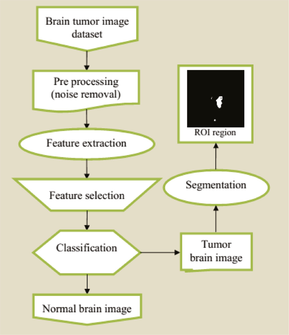
Overall Diagram of the Proposed MRI Brain Tumor Detection System.
3.1 Noise Removal
The noise removal of a MR image is a significant process of MRI tumor detection and segmentation. Consider the gray-scale input image Iin, which has a few of the noises like Gaussian noises, etc. The noise image certainly disturbs the output. So noise removal is a necessary part. By removing the noise from the image, there is better accuracy for the classification stage. In this work, in the noise-removal stage, we utilized the Gaussian filter, which is used to remove the noise from image Iin. Finally, we obtain the noise-free image I, which is used for further processing.
3.2 Feature Extraction
After the noise removal, the image is given to the feature-extraction stage. Feature extraction is an important stage for medical image classification. The beneficial features of the images are extracted from the image for classification purposes. To extract a good feature from the images is a challenging task. There are many feature-extraction techniques that are available. In this work, we extract GLCM and wavelet-based GLCM features from the images.
3.2.1 Feature Extraction Based on the Gray-Level Co-occurrence Matrix (GLCM)
The GLCM is utilized to extract the texture in an image by doing the transition of gray level within two pixels. The GLCM provides a joint distribution of gray-level pairs of neighboring pixels within an image. The co-occurrence matrix of the MR image is utilized to detect the tumor image. For the computation of GLCM, first a spatial relationship is recognized within two pixels; one is the reference pixel, and the other is a neighbor pixel. At this time, we compute the 22 features associated with GLCM. This process forms the GLCM containing a different combination of pixel gray values in an image. Let p(x, y) be the element of GLCM of a given image I of size m×n containing the number of gray levels GL ranging from 0 to GL−1. Table 1 shows the GLCM feature used in the proposed brain tumor detection system.
GLCM Feature Used in the Proposed Brain Tumor Detection System.
| Feature descriptor | Feature name | Computation |
|---|---|---|
| F1 | Angular second moment | |
| F2 | Contrast | |
| F3 | Inverse difference moment | |
| F4 | Entropy | |
| F5 | Correlation | |
| F6 | Variance | |
| F7 | Sum average | |
| F8 | Sum variance | |
| F9 | Sum entropy | |
| F10 | Difference entropy | |
| F11 | Inertia | |
| F12 | Cluster shade | |
| F13 | Cluster prominence | |
| F14 | Dissimilarity | |
| F15 | Homogeneity | |
| F16 | Energy | |
| F17 | Autocorrelation | |
| F18 | Maximum probability | |
| F19 | Inverse difference normalized (INN) | |
| F20 | Inverse difference moment normalized | |
| F21 | Information measure of correlation 1 | |
| F22 | Information measure of correlation 2 |
3.2.2 Feature Extraction via Wavelet-Based GLCM
In this section, at first, we apply the wavelet transform to the original image I. Here, we obtain the four subbands, which have low-frequency information and high-frequency information such as LL, LH, HL, and HH. Then, we calculate the GLCM feature for high-frequency subbands because the detail coefficients are available in the horizontal, vertical, and diagonal subbands. Then, the extracted 22 features are also extracted from these three bands. Finally, we obtain 88 features for one image: 66 wavelet GLCM features and 22 GLCM features.
3.3 Feature Selection Using OFPA
After calculating the features, we have to decrease the dimension of the feature vector because a high number of features are a great obstacle for classification. Consequently, a feature dimension-reduction technique is applied to reduce the features’ space without losing information. We decrease the number of features and take away the unrelated, redundant, or noisy information. In our work, we developed the OFPA algorithm for selecting the optimal features from the feature vector. The following steps are used to select the features.
Step 1: Solution Representation
To optimize the features, the OFPA algorithm initially creates an arbitrary population of the solution. Solution creation is an important step of the optimization algorithm that helps to identify the optimal solution quickly. Each image has the n number of features; among them, we select optimal features. The selected features are used for solution generation. Let us assume that there is M flower or solution in the entire population, and each flower contains N pollen. The whole flower population is represented as S=(F1, F2,…, FM), where Fm is the mth flower, and m∈[1, M] is the order number of the flower in the population. Each flower is represented as Fm=(P1, P2,…, PN), where, Pn is the nth pollen (feature) in the mth flower, and n∈[1, N] is the pollen index. The initial solution representation is given in Table 2.
Initial Solution Format of OFPA.
| F1 | F2 | F3 | F4 | … | F23 | F24 | F25 | … | F70 | F71 | F72 | … | F88 | ||
| P1 | 1 | 1 | 0 | 1 | … | 0 | 1 | 1 | … | 0 | 1 | 0 | … | 1 | |
| P2 | 1 | 0 | 0 | 1 | … | 1 | 0 | 1 | … | 1 | 0 | 1 | … | 0 | |
| Si | |||||||||||||||
| Pn | 0 | 1 | 1 | 0 | … | 0 | 1 | 0 | … | 0 | 1 | 1 | … | 1 |
Step 2: Opposite Solution for FPA
Rendering to opposition-based learning (OBL) familiarized by Tizhoosh in 2005 [28], the current solution and its opposite solution are measured simultaneously to get a better approximation for the current solution. It is provided that an opposite pollen solution has a better chance to be closer to the worldwide optimal solution than random pollen solution. The opposite pollen positions (OSi) are entirely defined by constituents of Si.
where OPi=Li+Ui−Pi with OPi ∈[Li, Ui] is the position of the ith opposite pollen OPi. Now, we obtain two sets of initial solutions. These solutions are given in the next steps.
Step 3: Fitness Calculation
After generating the solution, the fitness function is evaluated. The selection of the fitness is a crucial aspect in the OFPA algorithm. It is used to evaluate the aptitude (goodness) of candidate solutions. Here, classification accuracy is the main criteria used to design a fitness function. The fitness computation is executed for each solution. For each iteration, the fitness is calculated using equation (2),
where TP represents the true positive, TN represents the true negative, FP represents the false positive, and FN represents the false negative.
Step 4: Update Solution Based on FPA
After the fitness calculation, we update the solution on the basis of flower pollen algorithm (FPA). The main target of a flower is basically reproduction by pollination. Flower pollination frequently associates with the transfer of pollen that frequently related to pollinators, like birds. The global pollination can be characterized mathematically as equation (3).
where,
Γ(λ) is the standard γ function, and this distribution is precise for considerable steps (g>0). The local pollination and flower constancy can be represented as
where,
Step 5: Termination Criteria
The algorithm discontinues its execution only if a maximum number of iterations is achieved, and the solution that is holding the best fitness value is selected. Once the best fitness is attained by means of the FPA algorithm, the selected feature is given to the classification stage.
3.3 Classification Stage
The selected features are given to the classification stage. In this classification, we used the DNN. An artificial neural network model with the multiple layers of the hidden units and outputs is termed DNNs. Moreover, it consists of both pre-training (using generative deep belief network or DBN) and fine-tuning stages in its parameter learning. The main aim of this paper is to train the features of images in the particular data set, i.e. to find the right weight that can be used to correctly classify the input features.
(i) Pre-training Stage Using a Deep Belief Network (DBN)
In the training stage, we use a DBN that is a deep architecture and a feed forward neural network, i.e. with numerous hidden layers. The instance of the DBN network is shown in Figure 2. At this time, the abridged features are provided to the input of the DBN. At this time, we implement the learned weights as the initial weights of the DBN; this weight is engaged for generatively pre-training a DNN. The DBN model permits the network to produce visible activations on the basis of its hidden units’ states, which characterizes the network belief. This layer comprises an input layer that encircles the input units (called visible unit v), L number of hidden layers, and at last, an output layer that has one unit for each class is measured. The parameters of a DBN are the weights Wi among the units of layers i−1 and i, the biases B(i) of layer i (note that there are no biases in the input layer). To prepare the parameters is one among the chief difficulties for training DNN. Currently, the random initialization results in an optimization algorithm to determine the poor local minima of the fault function resulting in low generalization. We implemented the restricted Boltzmann machine (RBM) to work out the above issue. A DBN can be investigated as a composition of simple learning modules by stacking them. This uncomplicated learning module is known as the RBMs.
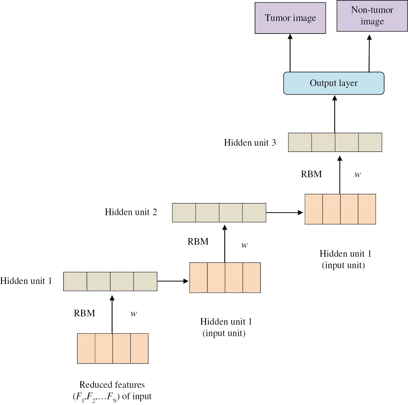
Proposed DBN with Three Hidden Layers.
Restricted Boltzmann Machine: An RBM is an exclusive type of Markov random field that has one layer of (typically Bernoulli) stochastic hidden units and one layer of (typically Bernoulli or Gaussian) stochastic visible or observable units. RBMs can be indicated as bipartite graphs, in which all visible units are connected to all hidden units, and there are no visible–visible or hidden–hidden connections. The important structure of RBM is quantified in Figure 3.
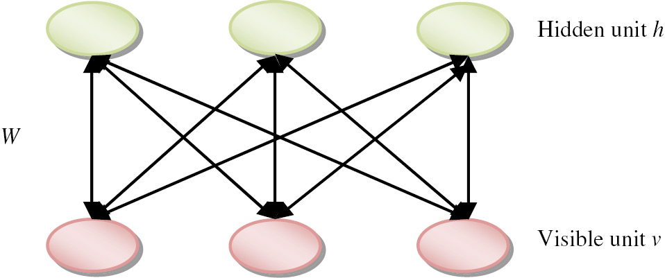
RBM Architecture.
In the training phase, primarily we analyze the energy performance of the visible layer v and the hidden layer h. A joint configuration (v, h) of the visible (Bernoulli) and hidden (Bernoulli) units of an RBM has an energy provided by:
where:
wij→ is the symmetric interaction term between the visible unit vi and the hidden unit hj,
ai, bj→ is the bias term,
I, J→ is the number of visible and hidden units.
By modifying the weights and biases to lower the energy of that information and to raise the energy of other information, the possibility that the network assigns to a training information can be raised principally for those that have low energies and, hence, make a big contribution to the partition function. The derivative of the log probability of a training vector concerning a weight is erratically easy. Between hidden units in an RBM, there are no direct influences; it is enormously easy to get an impartial sample of
where:
σ(x) → is the logistic sigmoid function
vihj → is the unbiased sample.
In addition, there are no direct connections among the visible units in an RBM. It is, furthermore, extremely uncomplicated to get an unbiased sample of the state of a visible unit, specified in a hidden vector
Then, the binary states of the hidden units are all computed in parallel using equation (7). Once the binary states have been chosen for the hidden units, a “reconstruction” is produced by setting each vi to 1 with a probability given by equation (8). Finally, the states of the hidden units are updated again. The change in a weight is then given by
where, under the distribution specified, the angle brackets are employed to indicate the expectations by the subscript that follows. For executing the stochastic steepest ascent in the log probability of the training data, this shows the way to a very uncomplicated learning rule
where:
η → is the learning rate.
Procedure for training the DNN:
Primarily we initialize the visible units v to the training vector.
After that, we update the hidden units in parallel in the provided visible units using equation (7).
In a similar manner, we update the visible units in parallel given the hidden units with the help of equation (8).
Then, we re-update the hidden units in parallel given the reconstructed visible unit with the help of the same equation utilized in step (9).
We accomplish the weight updates
When the RBM is trained, a dissimilar RBM can be “stacked” on top of it to form a multilayer model. Each time a dissimilar RBM is stacked, the input visible layer is a primed vector, and values for the units in the already-trained RBM layers are apportioned by means of the current weights and biases. The concluding layer of the already-trained layers is engaged as input to the novel RBM. The new RBM is then trained with the method above, and then, this complete procedure can be simulated until some needed stopping standard is met. We change the weight in each RBM for the purpose of declining the multi-objective function. The accomplished deep network weights are engaged in priming a fine-tuning phase.
(ii) Fine-Tuning Stage
After the network is pre-trained as the RBM–stack model, the weights are further attuned using back propagation for the purpose of upsurging the accuracy of the scheme. The fine-tuning phase is simply the ordinary back propagation algorithm. To categorize the tumor image, an output layer is intended (tumor or not) in the top of the DNN. Also, there are N number of input neurons (depending upon the features), and three hidden layers are utilized in our DNN. The optimized weight is intended through the training stage with the help of the training data set DT, where back propagation starts the weights attained in the pre-training phase. Primarily, the reduced features are provided to the DNN, though the weight is arbitrarily adjusted. The chief contribution of our DNN is to detect the minimum error function with the help of equation (6). Also, the training dataset is skilled until the optimized weight is grasped, or maximum accuracy is attained with the help of equation (6). Finally, on the basis of the optimal weight (w), the images are categorized in the testing stage by testing the data set DT.
3.5 Segmentation Stage
After the image classification stage, the tumor images are selected, and the selected images are given to the segmentation stage. In this work, for the segmentation stage, we utilize the PFCM. The application of the PFCM methods will improve the clustering process and the accuracy of the segmentation. The vital motive of the PFCM module is devoted to the segmentation of a specified set of data into clusters. The PFCM constitutes a data clustering technique, where each data point is a part of the cluster to a level indicated by the membership grade. In the clustering module, it is dependent on the reduction of the objective function, which is illustrated in the following equation (11):
where,
U → is the membership matrix,
T → is the possibilistic matrix,
C → is the resultant cluster center,
X → is the set of all data points.
The constants a and b represent the comparative significance of the fuzzy membership and typicality values in the objective function. The gradual procedure of the PFCM is effectively elucidated below.
Step 1: Calculation of Distance Matrix
At first, the number of clusters (C) is furnished by the user, which is identical with respect to every segment. When the number of clusters is determined, the evaluation of the distance between the centroids and data point for each segment is carried out. In this work, the Euclidian distance function is used for distance calculation. Further, the distance matrix is determined with respect to each and every cluster:
where ci is the centroid, and xk is the data point. Here, the distance function is effectively utilized to estimate the distance between every data point xk with every centroid vi value.
Step 2: Calculation of Typicality Matrix
After the estimation of the distance matrix, the typicality matrix is evaluated. The typicality matrix Tik is obtained from the possibilistic c-means (PCM) [20]. As illustrated in equation (13), the probability value of each data point in relation to every centroid is completed:
Step 3: Calculation of Membership Matrix
The evaluation of the membership matrix Uik is performed by means of assessing the membership value of the data point, which is gathered from the fuzzy c-means (FCM) [21]. As illustrated with the help of the following equation (14), the membership value of each data point in relation to each centroid is completed.
Step 4: Update of Centroid
After the generation of the clusters, the modernization of the centroids is performed in accordance with equation (15) shown below.
Subsequent to the modernization of the centroids with respect to each and every cluster, the task of evaluating the distance with the lately modernized centroids is started and continued until the evaluation of the modernization of the centroids. The relative procedure is performed again and again until the efficient centroids of each and every cluster become identical and similar in successive iterations.
Step 5: Stop the Whole Process
Using this PFCM, the input images are getting segmented. All the images are segmented, which means that we will stop the process.
4 Result and Discussion
In this section, we discuss the results obtained from the proposed brain tumor classification and segmentation technique. In implementing the proposed technique, we used Mat lab version (7.12). This proposed technique was done using Windows with an Intel Core i5 processor with speed 1.6 GHz and 4 GB RAM. The proposed system has been tested on the data set available on the Web. We have utilized the size of the image “512×512”, which is publicly available.
4.1. Evaluation Metrics
We need various assessment metric values to be calculated in order to analyze our proposed technique for the efficient MRI brain tumor classification. The metric values are found based on true positive (TP), true negative (TN), false positive (FP), and false negative (FN) with the option of segmentation and grading. The usefulness of our proposed work is analyzed by three metrics such as Accuracy, Sensitivity, and Specificity. The demonstration of these assessment metrics is specified in the equations that given below.
Sensitivity: The sensitivity of brain tumor detection is determined by taking the ratio of a number of true positives to the sum of true positive and false negatives. This relation can be expressed as:
Specificity: The specificity of the brain tumor detection can be evaluated by taking the relation of a number of true negatives to the combined true negative and the false positive. The specificity can be expressed as:
Accuracy: The accuracy of brain tumor detection can be calculated by taking the ratio of the true values present in the population. The accuracy can be described by the following equation:
4.2 MRI Data Set Description
The MRI brain image data set is effectively employed in the innovative image segmentation and classification techniques, which are obtained from the publicly accessible sources. The corresponding image data set contains 20 brain MRI images of which 15 brain images are with tumor and the remaining five brain images are without tumor. The brain image data set is subdivided into two distinct sets such as the training data set and the testing data set. The training data set is effectively utilized to segment the brain tumor images, and the testing data set is employed to evaluate the performance of the novel approach. Here, 10 images are elegantly employed for the training purpose, and the residual 10 images are effectively used for the testing purpose. Figure 4 illustrates certain sample MRI images with tumor and without tumor.
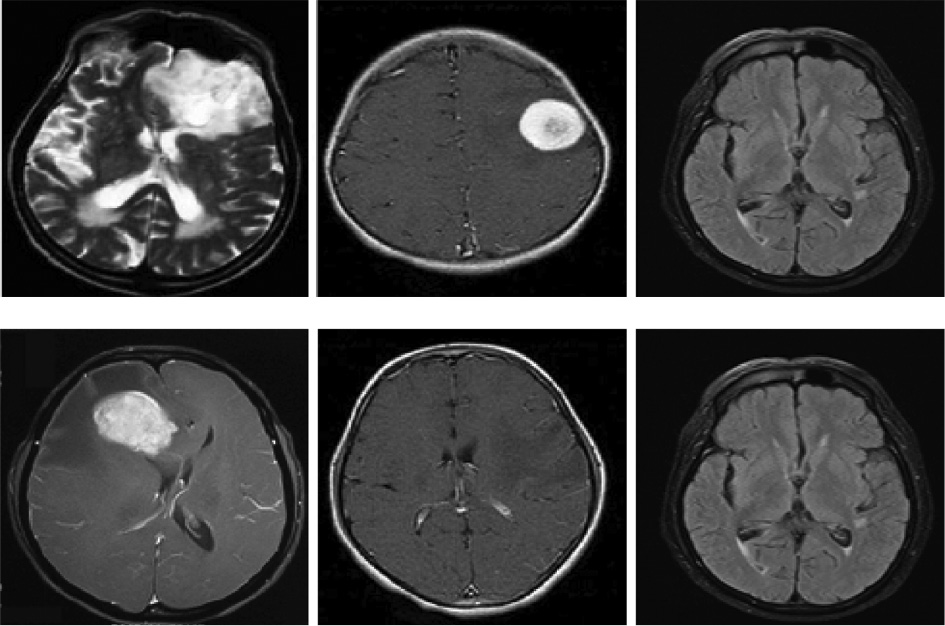
Sample Experimental Used Images.
4.3 Experimental Results on Proposed Approach
The performance of the proposed brain tumor classification and segmentation is analyzed with the help of sensitivity, specificity, and accuracy, which are the most significant performance parameters. The effectiveness of the proposed technique is demonstrated by performing a comparison between the matching results of the proposed method with other approaches. The result section is split into two phases, the classification phase and the segmentation phase. We first, verify the improvement of the classification phase. In the classification phase, we used the DNN classifier to recognize the tumor present in the image. In segmentation, we obtain the ROI and background region separately, and also, we measure the accuracy of the proposed approach with other segmentation approaches.
Performance of Classification Phase
The basic idea of our research is efficient MRI brain tumor detection and classification based on the combining wavelet texture feature and DNN. In the classification stage, at first, we extract the texture features from the image using GLCM and wavelet GLCM. After that, we reduce the features based on OFPA. Then, the relevant features are given to the DNN classifier for classification. Our proposed classification approach is compared with other well-known classifiers such as NN, RNN, and KNN. The performance of the approach is shown in Figures 5–7.
Figure 5 shows the performance of the accuracy plot based on the classification stage by varying hidden neuron sizes; as per the analysis, the accuracy gradually increases when compared to the other approaches. Here, in the classification stage, we used the DNN. In Figure 5, the hidden neuron size is 20. We obtain the maximum accuracy of 92% for using the proposed DNN, 70% for using NN, 70% for using RNN, and 60% for using KNN. Moreover, NN and RNN are producing almost the same output value. Moreover, Figure 6 shows the performance of the proposed approach based on sensitivity. Here, we also obtain the maximum accuracy compared to the other approaches. Similarly, Figure 7 shows the performance of the proposed approach based on specificity. In analyzing Figure 7, we obtain the maximum specificity of 100. From the three figures, we clearly understand that our proposed approach obtained better results compared to the existing approaches. Moreover, in this classification stage, we obtain the maximum accuracy because of the optimal feature selection using the OFPA methods. A large number of features are great obstacles for the classification stage. Here, oppositional based learning (OBL) is combined with the FPA algorithm to improve the performance.
Performance of Segmentation Phase
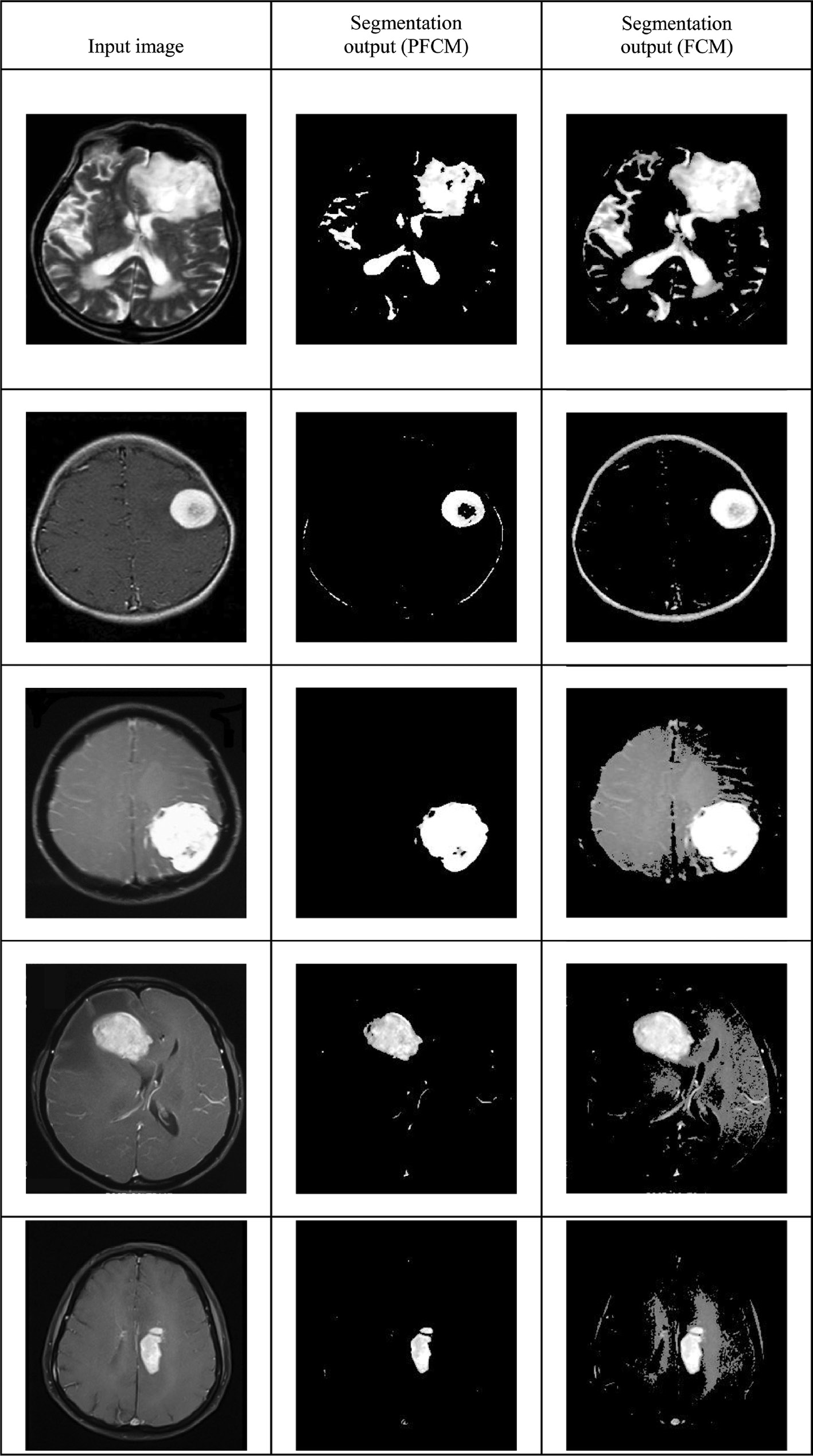
Segmentation is an important stage for tumor detection system. After the classification stage, the tumor images are given to the PFCM for segmentation. The explanation of the PFCM algorithm is explained in Section 3.5. The experimental results are illustrated in Table 3.
In this proposed methodology, for segmentation, we used the PFCM algorithm. This algorithm is a combination of the FCM and the PCM. Here, we compare our proposed PFCM algorithm with the FCM algorithm-based segmentation. Figure 8 shows the performance of the segmentation stage. Here, our proposed PFCM algorithm obtains the maximum output of 99.3%, 96.1%, and 99.5% for accuracy, sensitivity, and specificity, respectively. Moreover, the FCM-based segmentation approach achieves the output of 95.9%, 86%, and 87.2% for accuracy, sensitivity, and specificity, respectively. From the results, we clearly understand that our proposed PFCM algorithm outperforms the FCM algorithm. Moreover, Figure 9 shows the performance of the accuracy plot by varying the cluster size. Here, we obtain the maximum accuracy of 99.6%.
Compared with Published Paper
In this paper, we compare our proposed work with already published papers. Here, our proposed work was compared with the work of Kumar and Vijayakumar [17]. In Ref. [17], the author explained a tumor image segmentation and classification using the principal component analysis (PCA) and RBF kernel-based support vector machine. Here, the combined edge- and texture-based features are extricated using a histogram and the co-occurrence matrix, then, the PCA was depleted to demote the dimensionality of the feature space, which results in a more efficient and accurate classification. Finally, in the classification stage, a kernel-based SVM classifier was utilized to classify the image.
Table 4 shows the comparative analysis of the proposed methodology. Here, our proposed approach achieves the maximum accuracy of 92%, sensitivity of 865, and specificity of 91%. Similarly, using the work of Kumar and Vijayakumar [17], we obtain the accuracy of 88%, the sensitivity of 84%, and the specificity of 90%. From the discussion, we clearly understand that our proposed approach is better than the existing results.
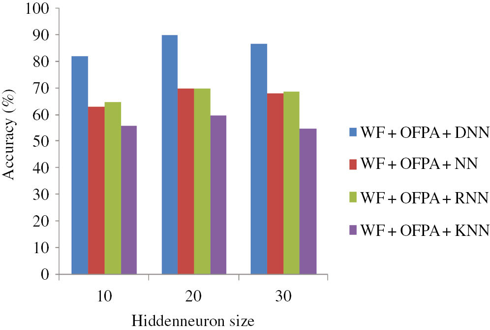
Performance of Proposed Approach Based on Accuracy.
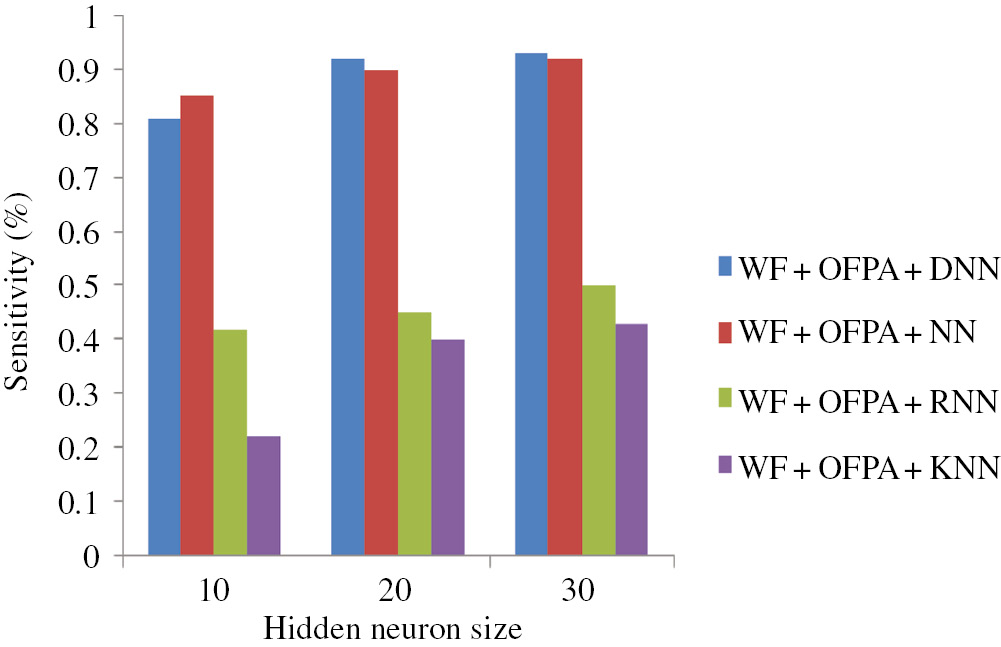
Performance of Proposed Approach Based on Sensitivity.
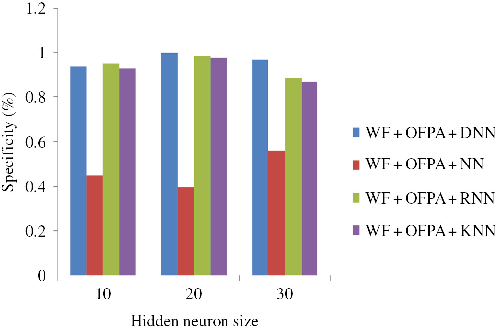
Performance of Proposed Approach Based on Specificity.
Experimental Results of Segmentation Stage.
 |
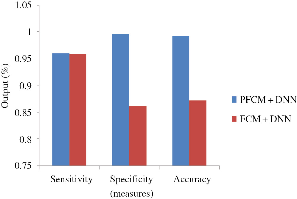
Performance of Segmentation Phase Using Different Measures.
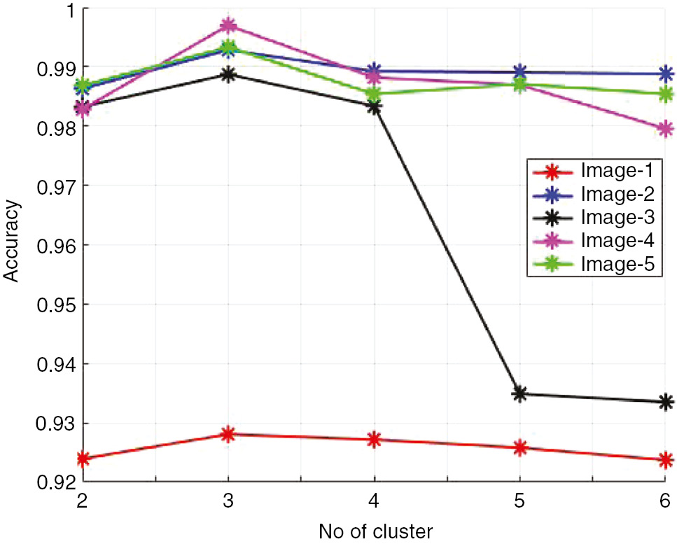
Performance of Accuracy Plot by Varying Cluster Size.
Comparative Analysis.
| Methods | Accuracy (%) | Sensitivity (%) | Specificity (%) |
|---|---|---|---|
| Kumar and Vijayakumar [17]. | 88 | 84 | 90 |
| Proposed | 92 | 86 | 91 |
5 Conclusion
In this paper, an efficient MRI tumor classification and segmentation process based on multiple stages was done. Our system comprised the following significant stages: preprocessing, feature extraction, feature selection, classification, and segmentation. At first, the noise present in the images was removed. Then, the important features are extracted, and the optimal feature is selected using the OFPA. In the classification stage, the tumor images are classified using the DNN. After the classification, the segmentation is done. The experimental results are explained, and our approach achieves the maximum accuracy compared to the existing approaches. Furthermore, in the future, a hybrid technique will be developed for the classification of the different types of tumors. Moreover, different data mining techniques can be used in training in order to improve the performance of the classifiers, and the data sets can also be increased.
Bibliography
[1] N. Acır, O. Ozdamar and C. Guzelis, Automatic classification of auditory brainstem responses using SVM-based feature selection algorithm for threshold detection, Eng. Appl. Artif. Intell.19 (2006), 209–218.10.1016/j.engappai.2005.08.004Search in Google Scholar
[2] S. M. Ali, L. K. Abood and R. S. Abdoon, Brain tumor extraction in MRI images using clustering and morphological operations techniques, Int. J. Geogr. Inf. Syst. Appl. Remote Sens.4 (2013), 12–25.Search in Google Scholar
[3] H. Almuallim and T. G. Dietterich, Learning with many irrelevant features, in: Proceedings of AAAI-91, pp. 547–552, 1991.Search in Google Scholar
[4] I. H. Bankman, Hand Book of Medical Image Processing and Analysis, Academic Press in Biomedical Engineering, 2009.Search in Google Scholar
[5] C. Blaiotta, M. Jorge Cardosob and J. Ashburner, Var. Inference Med. Image Segment.151 (2016), 14–28.10.1016/j.cviu.2016.04.004Search in Google Scholar
[6] A. L. Blum and P. Langley, Selection of relevant features and examples in machine learning, Artif. Intell.97 (1997), 245–271.10.1016/S0004-3702(97)00063-5Search in Google Scholar
[7] N. M. Borden and S. E. Forseen, Pattern Recognition Neuro Radiology, Cambridge University Press, New York, 2011.10.1017/CBO9781139042833Search in Google Scholar
[8] P. Domingos and M. Pazzani, On the optimality of the simple Bayesian classifier under zero-one loss, Mach. Learn.29 (1997), 103–130.10.1023/A:1007413511361Search in Google Scholar
[9] S. Dudoit, J. Fridlyand and T. P. Speed, Comparison of discrimination methods for the classification of tumors using gene expression data, J. Am. Stat. Assoc.97 (2002), 77–87.10.1198/016214502753479248Search in Google Scholar
[10] A. M. Fatih, Support vector machines combined with feature selection for breast cancer diagnosis, Expert Syst. Appl.36 (2009), 3240–3247.10.1016/j.eswa.2008.01.009Search in Google Scholar
[11] V. Grau, A. U. J. Mewes, M. Alcaniz, R. Kikinis and S. K. Warfield, Improved watershed transform for medical image segmentation using prior information, in: IEEE Trans. Med. Imaging23 (2004), 447–458.10.1109/TMI.2004.824224Search in Google Scholar PubMed
[12] M. Huang, W. Yang, Y. Wu, J. Jiang, W. Chen and Q. Feng, Brain tumor segmentation based on local independent projection-based classification, IEEE Trans Biomed. Eng.61 (2014), 2633–2645.10.1109/TBME.2014.2325410Search in Google Scholar PubMed
[13] M. A. Jaffar, A. Hussain, A. M. Mirza and A. Chaudhry, Fuzzy entropy and morphology based fully automated segmentation of lungs from CT scan images, Int. J. Innov. Comput. Inf. Control5 (2009), 4993–5002.10.1109/CIMCA.2008.168Search in Google Scholar
[14] K. Jong, J. Mary, A. Cornuejols, E. Marchiori and M. Sebag, Ensemble feature ranking, in: Proceedings Eur. Conference on Machine Learning and Principles and Practice of Knowledge Discovery in Databases, 2004.10.1007/978-3-540-30116-5_26Search in Google Scholar
[15] M. Karabatak and M. C. Ince, An expert system for detection of breast cancer based on association rules and neural network, Expert Syst. Appl.36 (2009), 3465–3469.10.1016/j.eswa.2008.02.064Search in Google Scholar
[16] J. Khan, J. S. Wei, M. Ringner, L. H. Saal, M. Ladanyi, F. Westermann, F. Berthold, M. Schwab, C. R. Antonescu, C. Peterson and P. S. Meltzer, Classification and diagnostic prediction of cancers using gene expression profiling and artificial neural networks, Nat. Med.7 (2001), 679.10.1038/89044Search in Google Scholar PubMed PubMed Central
[17] P. Kumar and B. Vijayakumar, Brain tumour MR Image segmentation and classification using by PCA and RBF kernel based support vector machine, Middle-East J. Sci. Res.23 (2015), 2106–2116.Search in Google Scholar
[18] L. Li, T. A. Darden, C. R. Weinberg, A. J. Levine and L. G. Pedersen, Gene assessment and sample classification for gene expression data using a genetic algorithm and k-nearest neighbor method, Comb. Chem. High Throughput Screen. 4 (2001), 727–739.10.2174/1386207013330733Search in Google Scholar PubMed
[19] Y. Li, F. Jia and J. Qin, Brain tumor segmentation from multimodal magnetic resonance images via sparse representation, J. Artif. Intell. Med.73 (2016), 1–13.10.1016/j.artmed.2016.08.004Search in Google Scholar PubMed
[20] Q. Liu, M. Jiang and P. Bai, A novel level set model with automated initialization and controlling parameters for medical image segmentation, Comput. Med. Imaging Graph.48 (2016), 21–29.10.1016/j.compmedimag.2015.12.005Search in Google Scholar PubMed
[21] D. Mahapatra, Combining multiple expert annotations using semi-supervised learning and graph cuts for medical image segmentation, Comput. Vis. Image Underst.151 (2016), 114–123.10.1016/j.cviu.2016.01.006Search in Google Scholar
[22] A. Osareh and B. Shadgar, A computer aided diagnosis system for breast cancer, Int. J. Comput. Sci.8 (2011), 233–235.Search in Google Scholar
[23] P. Sapra, R. Singh and S. Khurana, Brain tumor detection using neural network, Int. J. Sci. Mod. Eng. 1 (2013), 2319–6386.Search in Google Scholar
[24] D. Sridhar and M. Krishna, Brain tumor classification using discrete cosine transform and probabilistic neural network, in: International Conference on Signal Processing, Image Processing and Pattern Recognition, 2013.10.1109/ICSIPR.2013.6497966Search in Google Scholar
[25] G. Valentini, M. Muselli and F. Ruffino, Cancer recognition with bagged ensembles of support vector machines, Neurocomputing56 (2004), 461–466.10.1016/j.neucom.2003.09.001Search in Google Scholar
[26] H. Y. Yu and J. L. Fan, Three-level image segmentation based on maximum fuzzy partition entropy of 2-D histogram and quantum genetic algorithm, ICIC, LNAI5227 (2008), 484–493.10.1007/978-3-540-85984-0_58Search in Google Scholar
[27] Y. L. Zhang, N. Guo, H. Du and W. H. Li, Automated defect recognition of C- SAM images in IC packaging using Support Vector Machines, Int. J. Adv. Manuf. Technol.25 (2005), 1191–1196.10.1007/s00170-003-1942-1Search in Google Scholar
[28] S. Zhou, J. Wang and S. Zhang, Active contour model based on local and global intensity information for medical image segmentation, Neurocomputing186 (2016), 107–118.10.1016/j.neucom.2015.12.073Search in Google Scholar
©2019 Walter de Gruyter GmbH, Berlin/Boston
This article is distributed under the terms of the Creative Commons Attribution Non-Commercial License, which permits unrestricted non-commercial use, distribution, and reproduction in any medium, provided the original work is properly cited.
Articles in the same Issue
- Frontmatter
- Fusion Algorithm of Multi-focus Images with Weighted Ratios and Weighted Gradient Based on Wavelet Transform
- A Novel Approach to Extract Exact Liver Image Boundary from Abdominal CT Scan using Neutrosophic Set and Fast Marching Method
- A Fast Segmentation and Efficient Slice Reconstruction Technique for Head CT Images
- Fuzzy Approach to Decision Support System Design for Inventory Control and Management
- Multiple-Reservoir Scheduling Using β-Hill Climbing Algorithm
- Combining Wavelet Texture Features and Deep Neural Network for Tumor Detection and Segmentation Over MRI
- An Efficient Adaptive Filter for Fetal ECG Extraction Using Neural Network
- A Multi-Agents System for Solving Facility Layout Problem: Application to Operating Theater
- Global Research Trends of Intuitionistic Fuzzy Set: A Bibliometric Analysis
- Nurse Scheduling with Opposition-Based Parallel Harmony Search Algorithm
- Some Innovative Types of Fuzzy Ideals in AG-Groupoids
- Extracting Conceptual Relationships and Inducing Concept Lattices from Unstructured Text
- A Hybrid Cuckoo Search and Simulated Annealing Algorithm