A Novel Approach to Extract Exact Liver Image Boundary from Abdominal CT Scan using Neutrosophic Set and Fast Marching Method
-
Sangeeta K. Siri
 and
Mrityunjaya V. Latte
and
Mrityunjaya V. Latte

Abstract
Liver segmentation from abdominal computed tomography (CT) scan images is a complicated and challenging task. Due to the haziness in the liver pixel range, the neighboring organs of the liver have the same intensity level and existence of noise. Segmentation is necessary in the detection, identification, analysis, and measurement of objects in CT scan images. A novel approach is proposed to meet the challenges in extracting liver images from abdominal CT scan images. The proposed approach consists of three phases: (1) preprocessing, (2) CT scan image transformation to neutrosophic set, and (3) postprocessing. In preprocessing, noise in the CT scan is reduced by median filter. A “new structure” is introduced to transform a CT scan image into a neutrosophic domain, which is expressed using three membership subsets: true subset (T), false subset (F), and indeterminacy subset (I). This transform approximately extracts the liver structure. In the postprocessing phase, morphological operation is performed on the indeterminacy subset (I). A novel algorithm is designed to identify the start points within the liver section automatically. The fast marching method is applied at start points that grow outwardly to detect the accurate liver boundary. The evaluation of the proposed segmentation algorithm is concluded using area- and distance-based metrics.
1 Introduction
The liver is a vital organ that has many roles in the body, including building proteins and blood clotting, manufacturing triglycerides and cholesterol, glycogen synthesis, and bile production. The liver is the largest internal organ. Infections such as hepatitis, cirrhosis (scarring), cancer, and the overeffects of medications are identified diseases within the liver. The foremost stage for the computer-aided diagnosis of the liver is the identification of the liver region. Liver segmentation algorithms extract liver images from scan images, which helps in virtual surgery simulation and speeds up the disease diagnosis, accurate investigation, and surgery planning.
Liver segmentation from computed tomography (CT) scan images has gained a lot of importance in the medical image processing field because 1 in every 94 men and 1 in every 212 women born are susceptible to liver cancer in their lifetime [3, 14]. Liver cancer is one of the most common diseases, with increasing morbidity and high mortality [9, 33]. Liver cancer treatment requires maximum radiation dose to the tumor and minimum toxicity to the surrounding healthy tissues. This is the major challenge in clinical practice [25, 32]. Selective internal radiation therapy (SIRT) with yttrium-90 (Y-90) microspheres is an effective technique for liver-directed therapy [15]. SIRT dosimetry requires an accurate determination of the relative functional tumor(s) volume(s) with respect to the anatomical volumes of the liver to estimate the necessary Y-90 microsphere dose [4, 23]. Clinically, accurate liver volume determination is accomplished through tedious manual segmentation of the entire CT scan. A task is greatly dependent on the skill of the operator. Manual segmentation is time consuming. Thus, many automatic or semiautomatic techniques are available for segmentation and determine the volume of the liver accurately. This facilitates the operational process from a physician’s viewpoint.
Extracting liver from CT or magnetic resonance imaging (MRI) scan images is of prime importance. Considerable work has been done in extracting liver images from CT or MRI scan images, so a general solution has remained a challenge. Failure in getting a reliable and accurate segmentation algorithm is due to the following reasons: (1) The neighboring organs of the liver, such as the kidneys, heart, and stomach, have the same intensity level. (2) There is no definite shape, weight, size, volume, or texture for a liver. All these parameters are subjective. (3) The edges are weak. (4) The presence of artifacts in MRI or CT scan images. (5) Variability of liver geometry from patient to patient. (6) Large variation in pixel level range throughout the liver section as well as from patient to patient.
2 Related Work
Chen et al. [6] designed the Chan-Vese (C-V) model for liver segmentation in which the Gaussian function is used to find liver likelihood images from CT scan images and obtain the liver boundary using the C-V model. They have used morphological operation to improve the results. Song et al. [31] proposed an automatic liver boundary marking method based on an adaptive fast marching method (FMM). The liver image is separated from the CT scan by manually fixing the pixel intensity between 50 and 200. Median filter is applied to reduce noise and the liver image is enhanced by sigmoidal function. In this, the image is converted into binary and FMM is applied to find liver boundary accurately. Wu et al. [33] developed a novel method for the automatic delineation of the liver on CT volume images using supervoxel-based graph cuts. This method integrates histogram-based adaptive thresholding, simple linear iterative clustering, and graph cuts algorithm. Moghbel et al. [21] proposed random walker-based framework. In this, the liver dome is automatically detected based on the location of the right lung lobe and ribcage area and the liver is extracted using the random walker method. Ding et al. [7] introduced a multiatlas segmentation approach with local decision fusion for fast automated liver (with/without abnormality) segmentation on CT angiography. Zheng et al. [37] designed a feature learning-based random walker method for liver segmentation using CT images. Four texture features are extracted and then classified to determine the probability corresponding to the test images. In this, seed points on the original test image are automatically selected. Peng et al. [24] designed a novel multiregion appearance-based approach with graph cuts to delineate the liver surface and a geodesic distance-based appearance selection scheme is introduced to use proper appearance constraint for each subregion. Platero and Tobar [26] proposed a new approach to segment the liver from the CT scan, which is the combination of low-level operations, an affine probabilistic atlas, and a multiatlas-based segmentation. Salman AlShaikhli et al. [27] presented a novel fully automatic algorithm for 3D liver segmentation in clinical 3D CT images based on the Mahalanobis distance cost function using an active shape model implemented on MICCAI-SLiver07 achieving accurate results. Lu et al. [19] developed liver segmentation using a 3D convolutional neural network and the accuracy of initial segmentation is increased with graph cut algorithm and the previously learned probability map. Li et al. [18] developed a technique to detect the liver surface, which includes the construction of a statistical shape model using principal component analysis. Euclidean distance transformation is used to obtain a coarse position in a source image. The accurate detection of the liver is obtained using the deformable graph cut method. Zheng et al. [36] designed a tree-like multiphase level set algorithm for segmentation based on the C-V model to detect objects in an image. The algorithm is effective for images that have subobjects in the region.
3 Neutrosophic Set (NS)
NS was introduced by Samarandache [28]. In the NS theory, every event has not only a certain degree of the truth but also a falsity degree with indeterminacy. These parameters are considered independent from each other [13, 22]. An entity {S} is considered with opposite {Anti-S} and neutrality {Neut-S}. The {Neut-S} and {Anti-S} are referred to as {Non-S} [1, 10, 11, 22].
To apply the concept of NS to image processing, the image should be transformed into the neutrosophic domain. Image P of size X*Y with K gray levels can be defined as three arrays of neutrosophic images described by three membership sets: T (true subset), I (indeterminate subset), and F (false subset). Therefore, a pixel P(i, j) in the image transferred into the neutrosophic domain can be represented by PNS={T(i, j), I(i, j), F(i, j)} or PNS=P(t, i, f). It means that the pixel is%t true,%i indeterminate, and%f false [29]. Here, t varies in T (white pixel set), i varies in I (noise pixel set), and f varies in F (black pixel set), which are defined as follows [22, 28]:
where G̅(i, j) is the local mean value of the pixel of the window and given by following equation:
d(i, j) is the absolute value of the difference between intensity G(i, j) and its local mean value G̅(i, j) and given as
G(i, j) is the intensity value of the pixel P(i, j); w is the size of the sliding window; G̅min and G̅max are the minimum and maximum of the local mean values of the image, respectively; and dmin and dmax are the minimum and maximum value of d(i, j) in the whole image.
4 FMM
In the intended method, Sethian’s FMM [30] has been used to track the evolution of an expanding front. In our case, a front is a closed 2D curve that separates the interior and exterior regions. Because the closed surface is a curve in 2D and the lattice is a pixel raster, the FMM assigns to the pixel the time at which the expanding curve hits the pixel. Hence, at a given point, the motion of the front is described by the equation known as the Eikonal equation [2, 30, 31]:
where V(x) is the arrival time of the front at point x and S(x) is the speed function of front at point x. Because the front cannot only be expanded, the arrival time V is single valued. We assume that S=0 everywhere. The FMM simply propagates the shortest distance to the boundary from starting point. The above Eikonal equation is discretized and solved with the upwind scheme. For 2D grids, S can be obtained as follows:
where d+ and d− are the standard forward and backward operators, respectively. We have taken [1 0; −1 0; 0 1; 0 −1] as the difference operator.
5 Methodology
5.1 Preprocessing Phase
The abdominal CT scan image is with a 1019×682 DICOM color format. First, convert the CT scan image into a grayscale image of size 512×512. Reduce the noise using median filter.
5.2 Map the CT Scan Image into NS Domain
Step 1: Crop random section of the liver image.
Step 2: Obtain true subset T and false subset F using bell function.
where Cxy is the intensity value of pixel (i, j) in the cropped image of the liver. Variables a–d are the parameters that determine the shape of the bell function as shown in Figure 1.

Bell Function.
The values of variables a–d are obtained using the histogram-based method as follows:
Obtain the histogram of the cropped liver section.
Find the local maxima of the histogram.
Calculate the mean of local maxima.
(10)Find the peak values greater than the mean of local maxima Pmax.
b is the initial peak value; c is the final peak value.
Find the standard deviation (SD) of the cropped section of the liver.
(11)where
Find the value of a and d as follows:
Step 3: Convert T and F into binary [34].
Tth and Fth are the thresholds in true subset (T) and false subset (F), respectively. These are also required to obtain the indeterminacy subset (I). A heuristic approach is used to find the thresholds in T and F.
Select an initial threshold t0 in T.
Separate T using t0 and obtain two new groups of pixels: T1 and T2. (μ1 and μ2 are the mean values of these two groups.)
Compute new threshold value
Repeat steps (ii)–(iv) until the difference of tn −tn−1 is smaller than ϵ (ϵ=0.001 in the experiments) in successive iterations. Then, threshold Tth is calculated by following substitution:
The above steps are repeated for finding Fth in false subset (F).
Step 4: Find the indeterminacy subset (I) [34, 35].
Homogeneity is related to local information and plays an important role in image segmentation. We can define homogeneity using the SD and discontinuity of the intensity. SD describes the contrast within a local region, whereas discontinuity represents the changes in gray levels. Objects and background are more uniform and blurry edges are gradually changing from objects to background. The homogeneity value of objects and background is larger than that of the edges. A randomly identified size D×D window centered at (x, y) is used for computing the SD of pixel (i, j):
where μxy is the mean of intensity values within the window and given by following equation:
The discontinuity of pixel P(i, j) is described by the edge value. We use Sobel operator to calculate the discontinuity.
where Gx and Gy are the horizontal and vertical derivative approximations.
Normalize the SD and discontinuity and define the homogeneity as
where Sdmax=max{Sd (x, y)} and Egmax=max{Eg (x, y)}
The indeterminacy I(x, y) is represented as
The value of I(x, y) has a range of 0–1. The more uniform the region surrounding a pixel results in the minimum value of the indeterminate pixel. The window size should be big enough to include enough local information but still be less than the distance between the two objects. We chose D=10 in all calculations.
Step 5: Convert T, F, and I into binary image.
Procedure to find value of ∝.
min=minimum {maximum values of each column in indeterminacy image (I)≠0}.
∝ is any value less than or equal to min.
In this step, a given image is divided into three parts: object (Obj), edge (Edge), and Background (Bkg). T(x, y) represents the degree of being an object pixel (Obj), I(x, y) is the degree of being an edge pixel (Edge), and F(x, y) is the degree of being a background pixel (Bkg) for pixel P(x, y). The three parts are defined as follows:
(17)(18)(19)
The objects and background are mapped to 0 and the edges are mapped to 1 in the binary image. The mapping function is as follows:
5.3 Postprocessing Phase
Step 1: Perform morphological operation on indeterminacy set (I). This is called the speed function.
Step 2: Initial contour identification. FMM requires an initial contour from which the evolution of contour starts to detect the object boundary. In this paper, an effective initialization approach for the segmentation of the liver for FMM is proposed. The following steps are designed.
Find out the centroid of the liver as (centx′, centy′).
Choose diff=20, which is chosen experimentally.
The Points (centx′, centy′), (centx′+diff, centy′), (centx′, centy′+diff), (centx′+diff, centy′+diff) positioned in the liver are chosen as the start points. These four start points are located within the liver section.
Step 3: Apply FMM, which detects the liver boundary in the CT scan.
The complete process of the proposed technique is depicted in Figure 2.

Flowchart of the Proposed Liver Segmentation Algorithm.
6 Experimental Results
The experimental data set contains 108 patients’ CT scan images, which are provided by M/S CT Scan Centre, Hubli, Karnataka, India. Each slice of the CT scan is a 1019×682 size color image.
The original CT scan image, filtered image, and cropped random section of the liver are shown in Figure 3A–C, respectively. The true subset, false subset, and indeterminacy subset are shown in Figure 3D–F, respectively. The object image, background image, and edge images are shown in Figure 3G–I, respectively. The homogeneity image, speed function, and initial contour within the liver section are shown in Figure 3J–L, respectively. The final liver boundary at final iteration, extraction of the liver from abdominal CT scan, and boundary of the liver in the CT scan image are shown in Figure 3M–O, respectively. The ground truth image is shown in Figure 3P.

Illustration of liver extraction from CT scan using proposed method.
(A) Original CT scan image, (B) median filter image, (C) cropped random section of the liver, (D) true subset image, (E) false subset image, (F) indeterminate image, (G) foreground image, (H) background image, (I) edge image, (J) homogeneity image, (K) speed function, (L) initial contour in speed function, (M) liver boundary, (N) extraction of the liver from the CT scan image, (O) liver with boundary in CT scan and (P) ground truth image.
Figure 4 illustrates the experimental results of the proposed method for four images: columns (a) input image (CT scan image), (b) edge image of the CT scan, (c) speed function of the liver image, (d) liver with boundary, and (e) ground truth image.

Experimental Results of the Proposed Method and Existing Models.
Columns (A) input image (CT scan image), (B) edge image of the CT scan, (C) speed function of the liver image, (D) liver with boundary, and (E) ground truth image.
7 Comparison to Existing Methods
In this section, the performance of the proposed method is compared to the C-V model of Chan et al. [5] with specifications: μ=0.1, number of iterations=170, and initial contour position=[330, 310; 340, 330].
Li et al. [17] demonstrated the segmentation process with the following specifications: μ=1.0, ε=1.0, time step=0.10, σ=4, initial contour position=[160, 220; 190, 240], number of iterations=10. This is called the level set evolution (LSE) model.
Li et al. [16] demonstrated the segmentation process with the following specifications: σ=3.0, ε=1.0, μ=1.0, time step=0.1, λ1=1.0, λ2=1.0, number of iterations=25, initial contour position in the liver=[160, 200; 180, 200]. This is called the region-scalable fitting (RSF) model.
The initial contour in the liver section identified in the C-V, LSE, and RSF models and the proposed method are shown in Figure 5A, D, G, and J, respectively. The intermediate results of the C-V, LSE, and RSF models and the proposed method are shown in Figure 5B, E, H, and K, respectively. The final segmentation results of the C-V, LSE, and RSF models and the proposed method are shown in Figure 5C, F, I, and L, respectively.

Liver segmentation results comparison between proposed method and existing methods.
(A, D, G, and J) Initial contour in the liver image for the C-V, LSE, and RSF models and the proposed method, respectively; (B, E, H, and K) intermediate results for the C-V, LSE, and RSF models and the proposed method, respectively; and (C, F, I, and L) final segmentation results for the C-V, LSE, and RSF models and the proposed method, respectively.
The liver and its neighboring organs have the same intensity level, and due to more noise, all three existing algorithms have limitations, resulting in the inaccurate detection of the liver section. The proposed methodology fully exploits the intensity distribution information by cropping a random section of the liver and its segmentation resulting in the successful separation of the liver image from its neighboring organs.
In the C-V, LSE, and RSF models, it is necessary to identify the initial contour manually and the number of iterations. These parameters will affect the segmentation results. However, in the proposed method, there is no need to identify the number of iterations and initial contour manually. Once the complete liver boundary is detected, the results will be displayed on the computer screen. Initial contour is identified without user intervention.
8 Liver Segmentation Evaluation Metrics
Image segmentation plays an imperative role in a wide range of applications. Evaluating the competitiveness of the segmentation algorithm for a specified application is obligatory to allow the proper selection of segmentation algorithm as well as to fine tune their arguments to achieve acceptable performance. Experimental “disagreement methods” are based on the availability of the reference segmented image, also named the ground truth image. The discrepancy between the segmented image by any algorithm and a ground truth image can be used to gauge the algorithm’s performance.
In this paper, distance- and area-based metrics are adopted to evaluate and validate the contour detection process. Segmentations are evaluated with respect to the ground truth image generated under expert supervision.
8.1 Distance-Based Metrics
For some segmentation tasks, the delineation of the boundary is critical and is the objective of the segmentation. In these situations, distance-based metrics are essential and used to quantify the distance between the segmentation generated boundary (test boundary) and the “true” boundary. The average symmetric surface distance (ASSD) and maximum symmetric surface distance (MSSD) are two approaches that are normally adopted under distance-based metrics. The “test” boundary is SSEG and the “true” boundary is SGT.
8.1.1 ASSD
ASSD is given in millimeters and based on the surface voxels of two segmentations of SSEG and SGT. Surface voxels are defined with at least one nonobject voxel within their 18 neighbors [12, 20]. For each surface voxel of SSEG, the Euclidean distance to the closest surface voxel of SGT is calculated using the approximate nearest-neighbor technique and stored [12, 20]. To provide the symmetry, the same process is applied from the surface voxels of SGT to SSEG. The ASSD is then defined as the average of all calculated distances, which is zero for perfect segmentation [20].
Let S(seg) denote the set of surface voxel of segmentation [20]. The short distance of a voxel v to S(SEG) is defined as
where |·| denotes the Euclidean distance [20]. The average symmetric surface is then given by
8.1.2 MSSD
MSSD is also given in millimeters and is determined similar to the previous metrics. It is also called the Haudorff distance [12]. Differences between both sets of surface voxels are determined using Euclidean distances and the maximum value yields the MSSD. For perfect segmentation, this distance is 0 [12].
MSSD is sensitive to outliers and offers the maximum error. This is required for applications such as surgical planning, where the worst case error is more important than average errors.
8.2 Area-Based Metrics
Some segmentation techniques are used to measure the area or volume of the object (e.g. area of the liver and volume of the liver for treatment planning). In these situations, area-based metrics are well known. Area-based metrics are used to compare the object enclosed by a segmentation boundary SSEG and the “true” boundary SGT. The two approaches that are used under area-based metrics are true positive fraction (TPF; sensitivity) and false negative fraction (FNF; specificity).
8.2.1 TPF
TPF is the area fraction in the “true” segmented boundary (SGT) that is also enclosed by the algorithm segmented boundary (SSEG) [8]. For perfect segmentation, TPF is supposed to be 1.
8.2.2 FNF
FNF is the area fraction enclosed by the “true” boundary (SGT) that was missed by the segmentation algorithm (SSEG) [8]. For perfect segmentation, FNF is supposed to be 0.
9 Discussion
The proposed design introduces a novel framework for liver segmentation from CT scan images based on NS and FMM. The novel algorithm is proposed to convert an abdominal CT scan image to an NS domain. An NS domain gives an approximate structure of the liver. A new scheme is designed to detect the start points within the liver section, which is the primary requirement of FMM. The start points evolves outwardly to detect the exact liver boundary in the CT scan image. The results obtained are compared to ground truth images.
To assess the superiority of the proposed method, two types of evaluation metrics are adopted: (1) area-based method (i.e. TPF and FNF) and (2) surface distance-based method (i.e. ASSD and MSSD). The proposed method is compared to the existing method and the comparison results for 108 CT scan images are shown in Figures 6–9k. The average ASSD, MSSD, TPF, and FNF for 108 CT scan images for the proposed method and existing algorithm are tabulated in Table 1.
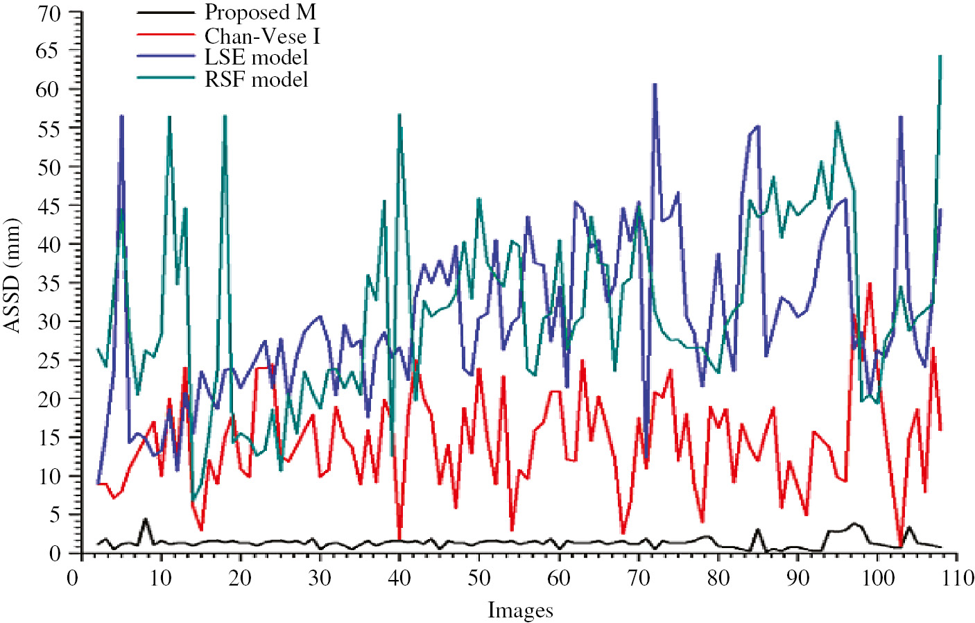
Comparison of Performance Evaluation Results using ASSD.

Comparison of Performance Evaluation Results using MSSD.

Comparison of Performance Evaluation Results using TPF.

Comparison of Performance Evaluation Results using FNF.
Average ASSD, MSSD, TPF and FNF for the Proposed Models and Existing Algorithm.
| C-V model | LSE model | RSF model | Proposed model | |
|---|---|---|---|---|
| ASSD (mm) | 14.3957±6.4248 | 30.2300±10.8651 | 31.6143±11.5892 | 1.3898±0.7205 |
| MSSD (mm) | 21.5573±6.7489 | 32.7687±10.7365 | 33.5736±10.9680 | 1.6047±0.9550 |
| TPF (%) | 41.8573±15.3772 | 37.8475±10.7340 | 41.0407±13.0454 | 91.6136±4.1388 |
| FNF (%) | 51.9265±14.5587 | 61.8413±11.3283 | 59.4688±12.9994 | 10.1079±3.0033 |
10 Conclusions
This paper designs a liver segmentation method implemented on CT scan images. NS is exploited to remove the neighboring structures of the liver and generated speed function. After locating the start points in speed function automatically, FMM is applied to find an outline of the liver image. This can be used for finding the area and volume of the liver, which helps the physician in liver disease diagnoses and liver transplantation. This can be applied to detect other anatomical structures of the abdomen, such as the kidneys and spleen, with minor modifications.
Bibliography
[1] N. Akhtar, N. Agarwal and A. Burjwal, K-mean algorithm for image segmentation using neutrosophy, in: Advances in Computing, Communications and Informatics (ICACCI), 2014 International Conference on, IEEE, New Delhi, India, 2014.10.1109/ICACCI.2014.6968286Search in Google Scholar
[2] N. Al Zaben, N. Madusanka, A. Al Shdefat and H.-K. Choi, Comparison of active contour and fast marching methods of hippocampus segmentation, in: Information and Communication Systems (ICICS), 2015 6th International Conference on, IEEE, Amman, Jordan, 2015.10.1109/IACS.2015.7103211Search in Google Scholar
[3] American Cancer Society, Cancer Facts & Figures, American Cancer Society, Atlanta, GA, USA, 2010.Search in Google Scholar
[4] R. Bhatt, M. Adjouadi, M. Goryawala, S. A. Gulec and A. J. McGoron, An algorithm for PET tumor volume and activity quantification: without specifying cameras point spread function (PSF), Med. Phys.39 (2012), 4187–4202.10.1118/1.4728219Search in Google Scholar PubMed
[5] T. Chan and L. A. Vese, Active contours without edges, IEEE Trans. Image Process.10 (2001), 266–277.10.1109/83.902291Search in Google Scholar PubMed
[6] Y. Chen, Z. Wang and W. Zhao, Liver segmentation in CT images using Chan-Vese model, in: 1st International Conference on Information Science and Engineering (ICISE2009), Nanjing, China, 2009.10.1109/ICISE.2009.718Search in Google Scholar
[7] X. Ding, C. Jiang, F. Tian, X. Yan, H. Qi, L. Zhang and Y. Zheng, Fast automated liver delineation from computational tomography angiography, Proc. Comput. Sci.90 (2016), 87–92.10.1016/j.procs.2016.07.028Search in Google Scholar
[8] A. Fenster and B. Chiu, Evaluation of segmentation algorithms for medical imaging, in: Proceedings of the 2005 IEEE Engineering in Medicine and Biology 27th Annual Conference, Shanghai, China, September 1–4, 2005.10.1109/IEMBS.2005.1616166Search in Google Scholar PubMed
[9] J. Ferlay, I. Soerjomataram, R. Dikshit, S. Eser, C. Mathers, M. Rebelo, D. M. Parkin, D. Forman and F. Bray, Cancer incidence and mortality worldwide: sources, methods and major patterns in GLOBOCAN 2012, Int. J. Cancer136 (2015), e359–e386.10.1002/ijc.29210Search in Google Scholar PubMed
[10] Y. Guo and H. D. Cheng, New neutrosophic approach to image segmentation, Pattern Recognit.42 (2009), 587–595.10.1016/j.patcog.2008.10.002Search in Google Scholar
[11] Y. Guo, H. D. Cheng, W. Zhao and Y. Zhang, A novel image segmentation algorithm based on fuzzy c-means algorithm and neutrosophic set, in: Proceeding of the 11th Joint Conference on Information Sciences, Atlantis Press, Shenzhen, China, 2008.10.2991/jcis.2008.44Search in Google Scholar
[12] T. Heimann, B. van Ginneken, M. A. Styner, Y. Arzhaeva, V. Aurich, C. Bauer, A. Beck, C. Becker, R. Beichel, G. Bekes, F. Bello, G. Binnig, H. Bischof, A. Bornik, P. Cashman, Y. Chi, A. Cordova, B. M. Dawant, M. Fidrich, J. D. Furst, D. Furukawa and L. Grena, Comparison and evaluation of methods for liver segmentation from CT datasets, IEEE Trans. Med. Imaging28 (2009), 1251–1265.10.1109/TMI.2009.2013851Search in Google Scholar
[13] A. Heshmati, M. Gholami and A. Rashno, Scheme for unsupervised colour-texture image segmentation using neutrosophic set and non-subsampled contourlet transform, IET Image Process.10 (2016), 464–473.10.1049/iet-ipr.2015.0738Search in Google Scholar
[14] A. Jemal, F. Bray, M. M. Center, J. Ferlay, E. Ward and D. Forman, Global cancer statistics, CA Cancer J. Clin.61 (2011), 69–90.10.3322/caac.20107Search in Google Scholar
[15] W. Y. Lau, S. Ho, T. W. T. Leung, M. Chan, R. Ho, P. J. Johnson and A. K. Li, Selective internal radiation therapy for nonresectable hepatocellular carcinoma with intraarterial infusion of 90yttrium microspheres, Int. J. Radiat. Oncol. Biol. Phys.40 (1998), 583–592.10.1016/S0360-3016(97)00818-3Search in Google Scholar
[16] C. Li, C.-Y. Kao, J. C. Gore and Z. Ding, Minimization of region-scalable fitting energy for image segmentation, IEEE Trans. Image Process.17 (2008), 1940–1949.10.1109/TIP.2008.2002304Search in Google Scholar PubMed PubMed Central
[17] C. Li, R. Huang, Z. Ding, J. C. Gatenby, D. N. Metaxas and J. C. Gore, A level set method for image segmentation in the presence of intensity inhomogeneities with application to MRI, IEEE Trans. Image Process.20 (2011), 2007–2016.10.1109/TIP.2011.2146190Search in Google Scholar PubMed PubMed Central
[18] G. Li, X. Chen, F. Shi, W. Zhu and J. Tian, Automatic liver segmentation based on shape constraints and deformable graph cut in CT images, IEEE Trans. Image Process.24 (2015), 5315–5329.10.1109/TIP.2015.2481326Search in Google Scholar PubMed
[19] F. Lu, F. Wu, P. Hu, Z. Peng and D. Kong, Automatic 3D liver location and segmentation via convolution neural network and graph cut, Int. J. Comput. Assist. Radiol. Surg.12 (2017), 171–182.10.1007/s11548-016-1467-3Search in Google Scholar PubMed
[20] J. Min, M. Powell and K. W. Bowyer, Automated performance evaluation of range image segmentation algorithms, IEEE Trans. Syst. Man Cybern. Pt. B Cybernet.34 (2004), 263–271.10.1109/TSMCB.2003.811118Search in Google Scholar
[21] M. Moghbel, S. Mashohor, R. Mahmud and M. I. Saripan, Automatic liver segmentation on computed tomography using random walkers for treatment planning, EXCLI J.15 (2016), 500.Search in Google Scholar
[22] J. Mohan, V. Krishnaveni and Y. Huo, Automated brain tumor segmentation on MR images based on neutrosophic set approach, in: IEEE Sponsored 2nd International Conference on Electronics and Communication System, Othakalmandapam, Coimbatore, India, ICECS, 2015.10.1109/ECS.2015.7124747Search in Google Scholar
[23] R. Murthy, R. Nunez, J. Szklaruk, W. Erwin, D. C. Madoff, S. Gupta, K. Ahrar, M. J. Wallace, A. Cohen, D. M. Coldwell, A. S. Kennedy and M. E. Hicks, Yttrium-90 microsphere therapy for hepatic malignancy: devices, indications, technical considerations, and potential complications, Radiographics25 (2005), S41–S55.10.1148/rg.25si055515Search in Google Scholar
[24] J. Peng, P. Hu, F. Lu, Z. Peng, D. Kong and H. Zhang, 3D liver segmentation using multiple region appearances and graph cuts, Med. Phys.42 (2015), 6840–6852.10.1118/1.4934834Search in Google Scholar
[25] G. C. Pereira, M. Traughber and R. F. Muzic, The role of imaging in radiation therapy planning: past, present, and future, BioMed Res. Int.2014 (2014), 231090.10.1155/2014/231090Search in Google Scholar
[26] C. Platero and M. C. Tobar, A multiatlas segmentation using graph cuts with applications to liver segmentation in CT scans, Comput. Math. Methods Med.2014 (2014), 182909.10.1155/2014/182909Search in Google Scholar
[27] S. D. Salman AlShaikhli, M. Y. Yang and B. Rosenhahn, 3D automatic liver segmentation using feature-constrained Mahalanobis distance in CT images, Biomed. Tech. Biomed. Eng.61 (2015), 401–412.10.1515/bmt-2015-0017Search in Google Scholar
[28] F. Samarandache, A unifying field in logics. Neutrosophic logic, in: Neutrosophy. Neutrosophic set, neutrosophic probability, 3rd ed., American Research Press, Rehoboth, USA, 2003.Search in Google Scholar
[29] G. I. Sayed, M. A. Ali, T. Gaber, A. E. Hassanien and V. Snasel, A hybrid segmentation approach based on neutrosophic sets and modified watershed: a case of abdominal CT Liver parenchyma, in: Computer Engineering Conference (ICENCO), 2015 11th International, Cairo, Egypt, IEEE, 2015.10.1109/ICENCO.2015.7416339Search in Google Scholar
[30] J. A. Sethian, Level set methods and fast marching methods, Cambridge University Press, Cambridge, England, 1999.10.1137/S0036144598347059Search in Google Scholar
[31] X. Song, M. Cheng, B. Wang and S. Huang, Automatic liver segmentation from CT images using adaptive fast marching method, in Seventh International Conference on Image and Graphics, Quigdao, China, 2013.10.1109/ICIG.2013.181Search in Google Scholar
[32] R. S. Stubbs, R. J. Cannan and A. W. Mitchell, Selective internal radiation therapy with 90yttrium microspheres for extensive colorectal liver metastases, J. Gastrointest. Surg.5 (2001), 294–302.10.1016/S1091-255X(01)80051-2Search in Google Scholar
[33] W. Wu, Z. Zhou, S. Wu and Y. Zhang, Automatic liver segmentation on volumetric CT images using supervoxel-based graph cuts, Comput. Math. Methods Med.2016 (2016), 1–14.10.1155/2016/9093721Search in Google Scholar PubMed PubMed Central
[34] M. Zhang, Novel approaches to image segmentation based on neutrosophic logic, Utah state university, USA, 2010.10.1016/j.sigpro.2009.10.021Search in Google Scholar
[35] M. Zhang, L. Zhang and H. D. Cheng, A neutrosophic approach to image segmentation based on watershed method, Signal Process.90 (2010), 1510–1517.10.1016/j.sigpro.2009.10.021Search in Google Scholar
[36] G. Zheng, H.-N. Wang and Y.-L. Li, A tree-like multiphase level set algorithm for image segmentation based on the Chan-Vese model, Acta Electron. Sin.34 (2006), 1508–1512.Search in Google Scholar
[37] Y. Zheng, D. Ai, P. Zhang, Y. Gao, L. Xia, S. Du, X. Sang and J. Yang, Feature learning based random walk for liver segmentation, PLoS One11 (2016), 1–17.10.1371/journal.pone.0164098Search in Google Scholar PubMed PubMed Central
©2019 Walter de Gruyter GmbH, Berlin/Boston
This article is distributed under the terms of the Creative Commons Attribution Non-Commercial License, which permits unrestricted non-commercial use, distribution, and reproduction in any medium, provided the original work is properly cited.
Articles in the same Issue
- Frontmatter
- Fusion Algorithm of Multi-focus Images with Weighted Ratios and Weighted Gradient Based on Wavelet Transform
- A Novel Approach to Extract Exact Liver Image Boundary from Abdominal CT Scan using Neutrosophic Set and Fast Marching Method
- A Fast Segmentation and Efficient Slice Reconstruction Technique for Head CT Images
- Fuzzy Approach to Decision Support System Design for Inventory Control and Management
- Multiple-Reservoir Scheduling Using β-Hill Climbing Algorithm
- Combining Wavelet Texture Features and Deep Neural Network for Tumor Detection and Segmentation Over MRI
- An Efficient Adaptive Filter for Fetal ECG Extraction Using Neural Network
- A Multi-Agents System for Solving Facility Layout Problem: Application to Operating Theater
- Global Research Trends of Intuitionistic Fuzzy Set: A Bibliometric Analysis
- Nurse Scheduling with Opposition-Based Parallel Harmony Search Algorithm
- Some Innovative Types of Fuzzy Ideals in AG-Groupoids
- Extracting Conceptual Relationships and Inducing Concept Lattices from Unstructured Text
- A Hybrid Cuckoo Search and Simulated Annealing Algorithm