A Fast Segmentation and Efficient Slice Reconstruction Technique for Head CT Images

2.1 Slice removal based on SSIM

Consider x={x_i|i=1, 2, …, N} and y={y_i|i=1, 2, …, N} as two discrete non-negative image signals with x_i and y_i representing the intensities of corresponding pixels in an image with window size N. The SSIM index [43] is,

where μx=1N∑i=1Nxi, σx=(1N−1∑i=1N(xi−μx)2)1/2,σxy=1N−1∑i=1N(xi−μx)(yi−μy),C1=(k1L)2, C2=(k2L)2, C3=C22 are constants inserted to avoid instability. μ_x, μ_y are the mean intensities of x and y, σ_xy is the covariance of x and y, and σ_x, σ_y are the standard deviations of x and y. k₁, k₂ are constants chosen to be ≪1. L is the dynamic range of pixel values.

The mean SSIM used to calculate the image quality of the entire image is given by,

where X and Y are the two images whose similarities are to be computed. x_j, y_j are the image contents at the jth local window, M is the number of samples in the quality map.

The extent of similarity between adjacent head CT slices in DICOM format is calculated using MSSIM. The process of slice selection from a set of hundreds of original head slices is done in two steps. First, a threshold is set for each five slices by averaging the similarity measures of these five slices. The slice that has a mean SSIM greater than the calculated threshold is discarded. Second, a further reduction in the ratio 2:1 is made just to show the effectiveness of the interpolation used. In order to rule out the possibility of organs disappearing in the selected slices, it is ensured that the number of slices discarded between two selected slices is limited to three. A uniform threshold is not practicable for medical images, as there is a possibility of sequential removal of slices, which may, in turn, lead to the missing details.

2.2 Iterative Phase-Field Segmentation Using Modified Allen-Cahn Equation

The phase-field model is a mathematical model for solving interfacial problems [3, 22]. The phase field or order parameter (ϕ) is used to separate one phase from the other. The edge-stopping function is calculated from the gradient image after normalization and Gaussian smoothing. The edge-stopping function plays a very vital role because this stops the evolution when the contour reaches the edge. The geometric ACM based on mean curvature motion using modified AC equation in the 2D domain Ω=(0, L_x)×(0, L_y) with x=(x, y) as its coordinate is given by:

where φ(x, t) is the phase-field function, f₀(x) is the normalized value of the given image f(x), g(f₀(x)) is the edge-stopping function, F(ϕ)=0.25(ϕ²−1)² is the double well potential function, Δφ(x, t) is the Laplacian operator, ϵ>0 is a constant called phase transition width (usually set to a value ≪1), and β is a parameter chosen as 50,000.

Consider the 2D space, Ω=(a, b)×(c, d) for discretization of equation (3). The uniform mesh size is given by Δx=(b−a)/N_x and Δy=(d−c)/N_y, where N_x, N_y are positive even integers. For simplicity, Δx=Δy=h. Let φijn be the approximation of φ(x_i, y_j, nΔt) with x_i=a+(i−0.5)h, y_j=(j−0.5)h as the cell centers and 1≤i≤N_x, 1≤j≤N_y·Δt=T/N_t, where T is the final time, and N_t is the total number of time steps. The discrete edge indicator function is given as:

where (G_σ∗f₀)_x,ij =[(G_σ∗f₀)_i+1,j −(G_σ∗f₀)_i−1,j ]/2h and (G_σ∗f₀)_y,ij =[(G_σ∗f₀)_i,j+1−(G_σ∗f₀)_i,j−1]/2h.

G_σ is the Gaussian function (σ=1.5). F(ϕ) takes 0.25 for ϕ=0 and zero for −1 and +1 values of ϕ. Zero Neumann boundary condition is used. Equation (3) is discretized as:

Δ_d is a discrete five point Laplacian operator. The multigrid method [4, 39] is a fast solver for solving discretized partial differential equations, and hence, Equation (5) is solved using a multigrid method with an initial condition φⁿ. The equation φt=gφ−φ3ϵ2 can be considered an approximation of Equation (6) and is solved using separation of variables with initial condition φⁿ=φ^∗, and the solution is given below:

The initial value of phase-field function is assigned to be 1 and −1 for values inside and outside the square contour. The square contour can be placed close to the object of interest by any initialization technique to speed up the evolution. Initially, F(φ) becomes zero in Equation (5), and after further iterations, φ takes a zero value on the boundary, −1 outside, and +1 inside the boundary. Equations (5) and (7) help in evolving the contour beyond non-convex and disconnected regions.

2.3 Proposed Phase-Field Segmentation

We hereby propose a PFS method for gray images by speeding up the simulation of IPFS (given in Section 2.2) by replacing the Laplacian term (Δdφij∗) used in Equation (5) by the term Δdφij∗−φij∗. The evolution of the contour is very fast without the need for any initialization technique irrespective of the image size or the region to be segmented, thereby, reducing the time taken for computation.

2.4 Re-creation of Omitted Slices Using Linear Interpolation

Re-creation is the reconstruction of omitted slices. Linear interpolation is applied to the selected segmented slices to reconstruct the missing slices. Consider N_s to be the number of slices, and φ(x, y, z_i) the segmented slice data with i=1, 2….N_s−1. Linear interpolation [27] is achieved using:

where 0≤θ≤1. Depending on the value of θ, the number of intermediate slices can be obtained. If θ=0.5, one slice will be created between two consecutive slices, if θ=0.33, two slices, if θ=0.25, three slices, and so on. Linear interpolation, even though computationally simple, creates blurred edges as it gives the weighted average of input slices.

2.5 Re-creation of Omitted Slices Using Registration-Based Interpolation

The REG-based interpolation algorithm uses non-rigid REG based on B-splines to preserve the spatial correspondence between adjacent slices. It deforms an image by manipulating a regular grid of control points based on a set of B-splines that are locally controlled. The similarity measure used to measure the degree of alignment between two images is the sum of the squared difference as the images are imaged using the same modality. REG is achieved by minimizing the cost function associated with the smoothness of transformation and image similarity. Using the non-rigid transformation and position of image plane created between two 2D slices, the interpolation directions between the two slices are defined. Optimization is carried using gradient descent algorithm. Generally, REG-based interpolation methods provide satisfactory results provided the organs in the slices taken as reference and template should not disappear, or the consecutive slices contain similar anatomical features. Additionally, the REG method should be capable of finding a suitable transformation map to match similar features. Violation of these might lead to false correspondence maps. The REG-based interpolation algorithm applied in this paper for comparison has been extensively reviewed in literature, and we refer the reader to Refs. [33] and [37] for more details.

2.6 Re-creation of Omitted Slices Using MCR-Based Interpolation

The energy functional E for MCR-based interpolation [2] is:

Let R₁ and R₂ be the two input images in the domain, Ω=(0, 1)×(0, 1), x be the grid of image values, S be the smoothness term, and u be the displacement value associated with each grid point that is to be determined. The ratio r=d₁/(d₁+d₂), where d₁ and d₂ are the distance from R to R₁ and R to R₂, where R is an arbitrary slice between R₁ and R₂. By considering r=0.5, the output slice is assumed to be in the middle of slices R₁ and R₂. For simplicity, the coefficient of u is assumed to be equal to 1 in Equation (10). However, this is not the case if more than one slice has to be re-created. α is a parameter to balance the smoothness of displacement and similarity of images. The sum of the squared difference is the distance measure D used, which is given by:

where Δ is the curvature operator. The use of curvature as the smoothness term eliminates the need for an affine linear mapping or the pre-REG step. To minimize E(u) in Equation (9), the derivative of E(u) is equated to zero, and a partial differential equation given below is obtained.

where A^curv[u]=Δ²u and f(x, u(x))=(R2(x+u)−R1(x−u))⋅(∇R1(x−u)+∇R2(x+u))(13)

To solve the PDE, a time-stepping iteration method with u⁰=0 and k≥0 is considered as

The discretized version of Equation (14) is

which is obtained using a finite difference approximation. l=1, 2 is the dimension index, τ is the time step, and I_n is the identity matrix. The solution to Equation (15) is efficiently realized [9, 10] using the discrete cosine transform (DCT). A set of coefficients for an image of size m×n with j₁=1, …m, j₂=1, …n can be computed using,

Defining G=DCT[U→l(k)+τF→l(k)], we have U→l(k+1)=IDCT[V], where Vj1,j2=Gj1,j2[1+ταdj1,j22]−1.

The intermediate slice R is obtained by averaging both the transformed input images (R₁, R₂) after the optimization process of calculating the final displacement field U→l(k+1).

The displacement field calculation for curvature-based REG with joint functional E(u)=D[R, T; u)]+αS is given as T(x−u(x))=R(x). Equation (9) is a modification of this equation in such a way that in MCR, the displacement field computed is applied to both R₁ and R₂, thereby, reducing the computational time needed for convergence. It is essential to note that in this work, as the number of slices to be re-created between the finalized slice set varies, d₁, d₂ and, consequently, r also varies.

3.1 Data

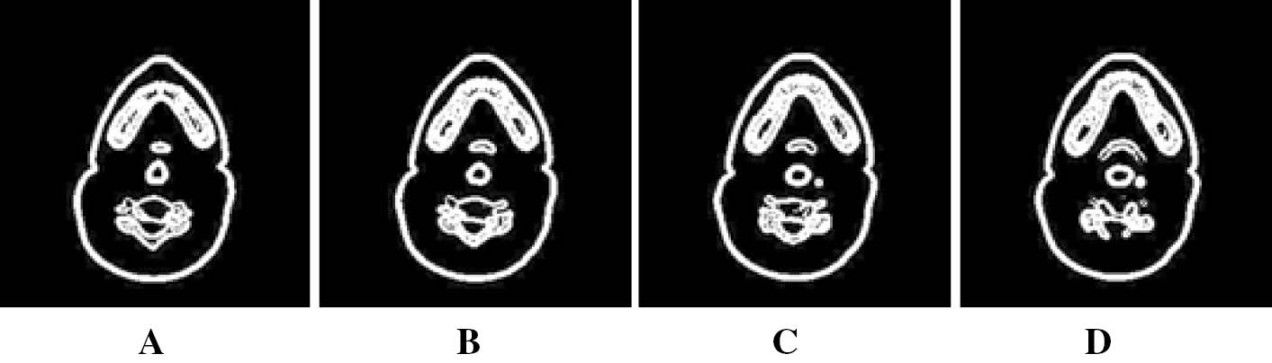
This study employs a collection of normal human head CT images taken from specialized and well-equipped scan center utilizing Siemens SOMATOM Sensation 64-slice CT scanner (Forchheim, Germany) (cardiac imaging with rotating time of 0.33 s and isotropic spatial resolution of 0.24 mm). The original images are in DICOM format, and we have chosen a test data of 100 slices for our implementation out of which the first four slices are shown in Figure 2. The current implementation was performed in MATLAB R2009b with Intel^® Pentium^® CPU B940 at 2 GHz, 4 GB RAM for an image size of 256∗256.

Figure 2:

Axial cross section of a human head CT-(A–D) corresponds to the first four slices respectively in DICOM format.

3.2 Quantitative Metrics for Evaluation

As the segments are solid and have high densities, performance metrics based on the four cardinalities are preferred, namely, accuracy (ACC), sensitivity (SEN), specificity (SPEC) along with MSE and PSNR [38] for the evaluation of both segmentation and interpolation methods. For the purpose of comparison, we perform PFS to all the 100 slices to deem them as ground truth (GT). True positive (TP) gives the number of pixels that are correctly detected as foreground, whereas false positive (FP) gives the number of pixels that are falsely detected as foreground. Similarly, true negative (TN) gives the number of pixels that are correctly detected as background, whereas false negative (FN) gives the number of pixels that are falsely detected as background.

Accuracy – It is the proportion of true results (both true positives and true negatives) in the population.

Accuracy=TP+TNTP+TN+FP+FN

Sensitivity – It is the proportion of positives measured as such.

Sensitivity=TPTP+FN

Specificity – It is the proportion of actual negatives, which are correctly identified as such.

Specificity=TNTN+FP

MSE – It measures the cumulative squared error between the interpolated/segmented (I) and the GT image with m, n as its dimensions.

MSE=1mn∑j1=0m−1∑j2=0n−1[I(j1, j2)− GT(j1, j2)]2

PSNR – It is a measure of reconstruction quality.

PSNR=10log10maximum intensity2MSE

3.3 Experimental Evaluation

Based on the mean SSIM, the intermediate and finalized slice selection performed is shown in Table 1 (for 25 slices), and the number of slices selected finally is only 10 out of 25. Correspondingly, only 31 slices are selected from a set of 100 slices. As a result, segmentation needs to be applied only to these 31 slices. This method helps in freeing up a lot of storage memory. We have chosen k₁=0.01, k₂=0.03 arbitrarily as the SSIM index algorithm is insensitive to these variations. The local window size chosen is 8×8.

The PFS model is compared against various deformable models in literature like ACM, CV model, GACM, distance regularized level set evolution (DRLSE), localized region-based ACM (LRAC), and the state-of-the art IPFS. The computational domain is set to Ω=(0, 1)×(0, 1) with h=1/128, time step Δt=4E−3, ϵ=0.03. The steady-state solution is obtained only if the relative error ||ϕn+1−ϕn||22/||ϕn||22 is less than the tolerance value (0.001) with the discrete l₂ norm of ϕh given by ||ϕh||2=∑h3(ϕijkn)2.Table 2 shows the average performance analysis of the different segmentation methods along with the time taken for 25 slices randomly selected from a set of 100 head CT slices. From the table, it is clear that the segmentation methods using IPFS and modified AC equation show greater accuracy and less MSE than other deformable models. However, the PFS method outperforms the IPFS in terms of the number of iterations and computational time even though the results of other evaluation metrics remain the same. Figure 3 shows the result of applying PFS to slices 1, 2, 3, and 4 of Figure 2.

Figure 3:

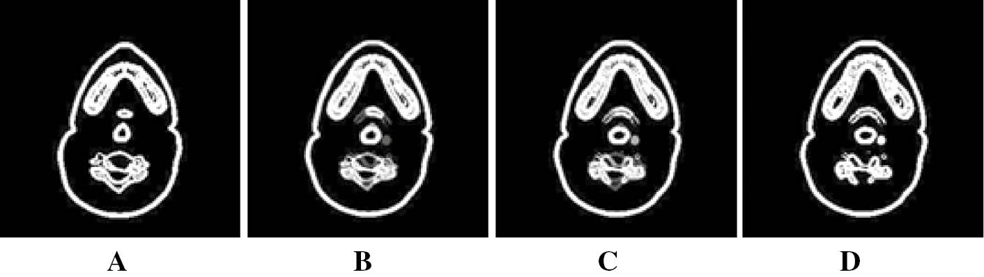
Phase Field segmented results of a human head CT. (A–D) corresponds to segmentation results of images in Figure 2.

However, when the focus is on the smooth 3D reconstruction of the human head from 2D slices, these 31 segmented slices will not suffice and it requires a greater number of slices. Interpolation helps in re-creating the discarded slices in between these 31 segmented slices. The average performance analysis for comparison of linear, REG-based interpolation and MCR interpolation for 100 slices are tabulated in Table 3. In the linear interpolation, averaging of the intensity values of the input slices is carried out which creates blurring on the edges as it does not consider the shape or structure information and, hence, is not suited for medical images.

The optimization parameter values chosen for the implementation of REG-based interpolation include a step size of 5, 2.5, 1.25 and a grid spacing of 8, 12 and 20 mm. The average time taken for REG-based interpolation is 162 s. The assumption that the objects within the input slices can only deform or move but cannot disappear should be taken into consideration, otherwise, the interpolation results become unpredictable. Moreover, this method is asymmetric as the values in the interpolated image differ depending on whether the reference image is matched to the template image or vice versa.

In the MCR-based interpolation method, the optimized displacement field for both horizontal and vertical directions is calculated, which helps in providing sharper and accurate results than linear and REG-based interpolation. We have chosen time step τ=0.05 and the regularization parameter α=100. The average computational time (30.73 s) for MCR interpolation is longer than the linear interpolation but less than the REG-based interpolation. For both REG- and MCR-based interpolation, iterations were stopped when the relative error was below 10⁻³. The reconstructed slices 2 and 3 between the two segmented selected slices 1 and 4 using linear, REG-based, and MCR-based interpolations are shown in Figures 4–6, respectively, for a subjective comparison. Also, it is important to note that the sensitivity (95.802%) is improved on par with specificity (95.901%) in the MCR interpolation along with the accuracy and PSNR with minimum MSE. The average performance analysis with respect to the number of slices re-created between the finalized segmented slice set using the interpolation methods discussed above is given in Table 4 for a more detailed understanding. As stated earlier, the number of slices re-created is limited to a maximum of three. As the number of slices re-created increases, there is a corresponding decrease in accuracy and PSNR with an increase in MSE. This is one of the reasons for limiting the number of slices to be re-created.

Figure 4:

Re-creation of slices using linear interpolation. (B and C) are re-created slices by applying linear interpolation to the selected segmented slices (A and D).

Figure 5:

Re-creation of slices using REG based interpolation. (B and C) are re-created slices by applying REG based interpolation to the selected segmented slices (A and D).

Figure 6:

Re-creation of slices using MCR based interpolation. (B and C) are re-created slices by applying MCR based interpolation to the selected segmented slices (A and D).

Figure 7 shows the graphical plot of the performance metrics for the different interpolation methods for a set of 100 slices compared against the ground truth. The slices 1, 4, 6, 9, 12 …, being selected segmented slices and are not interpolated, show an accuracy of 100% with zero MSE and infinite PSNR, which can be visualized in the graph. The X-axis represents the 100 interpolated data set samples, and the Y-axis represents the performance metrics for evaluation. Moreover, Figure 8 depicts the performance evaluation based on the low-, medium- and high-level similarity measure. The range of low and high is below 0.6 and above 0.7, and the medium level lies in between these. This approach of measurement helps in understand better that the performance evaluation results are highly dependent on the similarity measures.

Figure 7:

Graphs Showing Performance Analysis for Linear, Registration and MCR-based Interpolation.

Figure 8:

Bar Graph Showing Performance Analysis Based on Three Different Levels of SSIM.

(A) Low-level SSIM. (B) Medium-level SSIM. (C) High-level SSIM. (D) SSIM-based MSE.

It may be considered that even though time reduction is achieved in segmentation, additional time is added up during interpolation. However, it must be noted that reduction in the time of segmentation in itself is justified, and as interpolation is an independent activity, time consumption may be reduced by carrying out interpolation of different slice sets in parallel. The prime focus of this work is reducing the storage requirements, and the results demonstrate very well that the requirement of storage space may be reduced to around one third.

Bibliography

[1] H. Atoui, S. Miguet and D. Sarrut, A fast morphing based interpolation for medical images: application to conformal radiotherapy, Image Anal. Stereol.25 (2006), 95–103.10.5566/ias.v25.p95-103Search in Google Scholar
[2] A. Baghaie and Z. Yu, Curvature-based registration for slice interpolation of medical images, computational modeling of objects presented in images fundamentals, methods, and applications, pp. 69–80, Springer International Publishing, Cham, 2014.10.1007/978-3-319-09994-1_7Search in Google Scholar
[3] M. Benes, V. Chalupecky and K. Mikula, Geometrical image segmentation by the Allen-Cahn equation, Appl. Numer. Math.51 (2004), 187–205.10.1016/j.apnum.2004.05.001Search in Google Scholar
[4] W. L. Briggs, A multigrid tutorial, SIAM, Philadelphia, Pennsylvania, 1987.Search in Google Scholar
[5] V. Caselles, R. Kimmel and G. Sapiro, Geodesic active contours, Int. J. Comput Vis.22 (1997), 61–79.10.1023/A:1007979827043Search in Google Scholar
[6] T. F. Chan and L. A. Vese, Active contour without edges, IEEE Trans. Image Process.10 (2001), 266–277.10.1109/83.902291Search in Google Scholar PubMed
[7] J. Cheng and X. Sun, Medical image segmentation with improved gradient vector flow, Res. J. Appl. Sci. Eng. Technol.4 (2012), 3951–3957.Search in Google Scholar
[8] W. R. Crum, T. Hartkens and D. L. G. Hill, Non-rigid image registration: theory and practice, Br. J. Radiol.77 (2004), S140–S153.10.1259/bjr/25329214Search in Google Scholar PubMed
[9] B. Fischer and J. Modersitzki, Curvature based image registration, J. Math. Imaging Vis.18 (2003), 81–85.10.1023/A:1021897212261Search in Google Scholar
[10] B. Fischer and J. Modersitzki, A unified approach to fast image registration and a new curvature based registration technique, Linear Algebra Appl.380 (2004), 107–124.10.1016/j.laa.2003.10.021Search in Google Scholar
[11] D. H. Frakes, L. P. Dasi, K. Pekkan, H. D. Kitajima, K. Sundareswaran, A. P. Yoganathan and M. J. T. Smith, A new method for registration-based medical image interpolation, IEEE Trans. Med. Imaging27 (2008), 370–377.10.1109/TMI.2007.907324Search in Google Scholar PubMed
[12] B. Girod, What’s wrong with mean-squared error, in: A. B. Watson, ed., Digital images and human vision, pp. 207–220, The MIT Press, Cambridge, MA, 1993.Search in Google Scholar
[13] G. J. Grevera and J. K. Udupa, Shape-based interpolation of multidimensional grey-level images, IEEE Trans Med. Imaging15 (1996), 881–892.10.1109/42.544506Search in Google Scholar PubMed
[14] G. J. Grevera and J. K. Udupa, An objective comparison of 3-D image interpolation methods, IEEE Trans Med. Imaging17 (1998), 642–652.10.1109/42.730408Search in Google Scholar PubMed
[15] L. Hi, Z. Peng, B. Everding, X. Wang, C. Y. Han, K. L. Weiss and W. G. Wee, A comparative study of deformable contour methods on medical image segmentation, Image Vis. Comput.26 (2008), 141–163.10.1016/j.imavis.2007.07.010Search in Google Scholar
[16] D. L. G. Hill, P. G. Batchelor, M. Holden and D. J. Hawkes, Medical image registration, Phys. Med. Biol.46 (2001), R1–R45.10.1088/0031-9155/46/3/201Search in Google Scholar PubMed
[17] M. Kass, A. Witkin and D. Terzopoulos, Snakes: active contour models, Proc. IEEE Int. Conf. Comput. Vis.259 (1987), 261–268.10.1007/BF00133570Search in Google Scholar
[18] S. Lankton and A. Tannenbaum, Localizing region-based active contours, IEEE Trans. Image Process. 17 (2008), 2029–2039.10.1109/TIP.2008.2004611Search in Google Scholar PubMed PubMed Central
[19] T. Y. Lee and C. H. Lin, Feature-guided shape-based image interpolation, IEEE Trans. Med. Imaging21 (2002), 1479–1489.10.1109/TMI.2002.806574Search in Google Scholar PubMed
[20] T. Y. Lee and W. H. Wang, Morphology-based three dimensional interpolation, IEEE Trans Med. Imaging19 (2000), 711–21.10.1109/42.875193Search in Google Scholar PubMed
[21] J. Leng, G. Xu and Y. Zhang, Medical image interpolation based on multi-resolution registration, Comput. Math. Appl.66 (2013), 1–18.10.1016/j.camwa.2013.04.026Search in Google Scholar
[22] Y. Li and J. Kim, A fast and accurate numerical method for medical image segmentation, J. Korean Soc. Industr. Appl. Math.14 (2010), 201–210.Search in Google Scholar
[23] Y. Li and J. Kim, Multiphase image segmentation using a phase-field model, Comput. Math. Appl.62 (2011), 737–745.10.1016/j.camwa.2011.05.054Search in Google Scholar
[24] Y. Li and J. Kim, An unconditionally stable numerical method for bimodal image segmentation, Appl. Math. Comput.219 (2012), 3083–3090.10.1016/j.amc.2012.09.038Search in Google Scholar
[25] C. Li, C. Xu, C. Gui and M. D. Fox, Distance regularized level set evolution and its application to image segmentation, IEEE Trans. Image Process.19 (2010), 3243–3254.10.1109/TIP.2010.2069690Search in Google Scholar
[26] Y. Li, H. G. Lee, D. Jeong and J. Kim, An unconditionally stable hybrid numerical method for solving the Allen–Cahn equation, Comput. Math. Appl. 60 (2010), 1591–1606.10.1016/j.camwa.2010.06.041Search in Google Scholar
[27] Y. Li, J. Shin, Y. Choi and J. Kim, Three-dimensional volume reconstruction from slice data using phase field models, Comput. Vis. Image Underst.137 (2015), 115–124.10.1016/j.cviu.2015.02.001Search in Google Scholar
[28] J. B. Maintz and M. A. Viergever, A survey of medical image registration, Med. Image Anal.2 (1998), 1–36.10.1016/S1361-8415(98)80001-7Search in Google Scholar
[29] T. McInerney and D. Terzopoulos, Deformable models in medical image analysis: a survey, Med. Image Anal.1 (1996), 91–108.10.1016/S1361-8415(96)80007-7Search in Google Scholar
[30] J. Modersitzki, Numerical methods for image registration, numerical mathematics and scientific computation, Oxford University Press, New York, NY, 2004.10.1093/acprof:oso/9780198528418.001.0001Search in Google Scholar
[31] W. J. Niessen, B. M. ter Haar Romeny and M. A. Viergever, Geodesic deformable models for medical image analysis, IEEE Trans. Med. Imaging17 (1998), 634–641.10.1109/42.730407Search in Google Scholar PubMed
[32] A. Norouzi, M. Shafry, M. Rahim, A. Altameem, T. Saba, A. E. Rad, A. Rehman and M. Uddin, Medical image segmentation methods, algorithms, and applications, IETE Tech. Rev. 31 (2014), 199–213.10.1080/02564602.2014.906861Search in Google Scholar
[33] G. P. Penney, J. A. Schnabel, D. Rueckert, M. A. Viergever and W. J. Niessen, Registration-based interpolation, IEEE Trans. Med. Imaging23 (2004), 922–926.10.1109/TMI.2004.828352Search in Google Scholar PubMed
[34] D. L. Pham, C. Xu and J. L. Prince, Current methods in medical image segmentation, Annu. Rev. Biomed. Eng.2 (2000), 315–337.10.1146/annurev.bioeng.2.1.315Search in Google Scholar PubMed
[35] L. Qin, C. Zhu, Y. Zhao, H. Bai and H. Tian, Generalized gradient vector flow for snakes: new observations, analysis and improvement, IEEE Trans. Circuits Syst. Video Technol.23(5) (2013), 883–897.10.1109/TCSVT.2013.2242554Search in Google Scholar
[36] S. P. Raya and J. K. Udupa, Shape-based interpolation of multidimensional objects, IEEE Trans. Med. Imaging9 (1990), 32–42.10.1109/42.52980Search in Google Scholar PubMed
[37] D. Rueckert, L. Sonoda, C. Hayes, D. Hill, M. Leach and D. Hawkes, Non-rigid registration using free-form deformations: application to breast MR images, IEEE Trans. Med. Imaging18 (1999), 712–721.10.1109/42.796284Search in Google Scholar PubMed
[38] A. A. H. Thasneem, R. Mehaboobathunnisa, M. M. Sathik and S. Arumugam, Comparison of different segmentation algorithms for dermoscopic images, ICTACT J. Image Video Process.05 (2015), 1030–1036.10.21917/ijivp.2015.0151Search in Google Scholar
[39] U. Trottenberg, C. Oosterlee and A. Schüller, Multigrid, Academic Press, San Diego, CA, 2001.Search in Google Scholar
[40] Z. Wang, The SSIM index for image quality assessment. http://www.cns.nyu.edu/∼lcv/ssim/.Search in Google Scholar
[41] Z. Wang and A. C. Bovik, A universal image quality index, IEEE Signal Process. Lett.9 (2002), 81–84.10.1109/97.995823Search in Google Scholar
[42] Z. Wang, A. C. Bovik and L. Lu, Why is image quality assessment so difficult, Proc. IEEE Int. Conf. Acoust. Speech Signal Process.4 (2002), 3313–3316.10.1109/ICASSP.2002.5745362Search in Google Scholar
[43] Z. Wang, A. C. Bovik, H. R. Sheikh and E. P. Simoncelli, Image quality assessment: from error measurement to structural similarity, IEEE Trans. Image Process.13 (2004), 600–612.10.1109/TIP.2003.819861Search in Google Scholar PubMed
[44] C. Xu and J. Prince, Snakes, shapes, and gradient vector flow, IEEE Trans. Image Process.7 (1998), 359–369.10.1109/83.661186Search in Google Scholar PubMed
©2019 Walter de Gruyter GmbH, Berlin/Boston
This article is distributed under the terms of the Creative Commons Attribution Non-Commercial License, which permits unrestricted non-commercial use, distribution, and reproduction in any medium, provided the original work is properly cited.
Articles in the same Issue
- Frontmatter
- Fusion Algorithm of Multi-focus Images with Weighted Ratios and Weighted Gradient Based on Wavelet Transform
- A Novel Approach to Extract Exact Liver Image Boundary from Abdominal CT Scan using Neutrosophic Set and Fast Marching Method