A Hybrid Cuckoo Search and Simulated Annealing Algorithm

Faisal Alkhateeb; Bilal H. Abed-alguni

doi:10.1515/jisys-2017-0268

Article Open Access

A Hybrid Cuckoo Search and Simulated Annealing Algorithm

Faisal Alkhateeb and Bilal H. Abed-alguni

Published/Copyright: October 5, 2017

Published by

Become an author with De Gruyter Brill

Submit Manuscript Author Information

From the journal Journal of Intelligent Systems Volume 28 Issue 4

Abstract

Simulated annealing (SA) proved its success as a single-state optimization search algorithm for both discrete and continuous problems. On the contrary, cuckoo search (CS) is one of the well-known population-based search algorithms that could be used for optimizing some problems with continuous domains. This paper provides a hybrid algorithm using the CS and SA algorithms. The main goal behind our hybridization is to improve the solutions generated by CS using SA to explore the search space in an efficient manner. More precisely, we introduce four variations of the proposed hybrid algorithm. The proposed variations together with the original CS and SA algorithms were evaluated and compared using 10 well-known benchmark functions. The experimental results show that three variations of the proposed algorithm provide a major performance enhancement in terms of best solutions and running time when compared to CS and SA as stand-alone algorithms, whereas the other variation provides a minor enhancement. Moreover, the experimental results show that the proposed hybrid algorithms also outperform some well-known optimization algorithms.

Keywords: Cuckoo search; simulated annealing search; optimization; metaheuristic

MSC 2010: 68T01

1 Introduction

Cuckoo search (CS) is a recent population-based optimization algorithm [30] that can be used for optimizing discrete and continuous problems. CS is distinguished from other optimization algorithms by the use of a randomization method based on Lévy flight and the use of one insensitive tuning parameter [20], [23], [30], [31].

On the contrary, simulated annealing (SA) is a single-solution search algorithm that can be used for optimizing discrete [9], continuous, and statistical combinatorial problems [14]. CS and SA are iterative algorithms that generate solutions based on a random method and replace the current solutions by better ones. Unlike CS and some local search algorithms (see Ref. [12] for Hill-climbing algorithm), SA increases the chance of avoiding local optima because it explores the solution space and allows replacing current solutions by worse ones with a decreasing probability [12], [28].

Recently, several researchers have attempted to hybridize SA with other techniques to solve different types of optimization problems [13], [25], [26]. Liu and Wang [13] used the SA algorithm with some priority rules to solve the problem of cellular manufacturing system (CMS) with dual-resource constrained setting. The SA algorithm with some parallel operators and constraints has been used by Shivasankaran et al. [25] to solve the repair shop job sequencing and operator allocation problem. Shivasankaran et al. [26] proposed a hybrid sorting immune SA algorithm to solve the flexible job-shop scheduling problem. The SA algorithm has been combined with differential evolution algorithms to solve joint replenishment and delivery problem with trade credit [33].

Similar to many other optimization algorithms, CS suffers from the problem of premature convergence and the problem of slow convergence especially when it is used to solve complex optimization problems [2]. Therefore, many research studies have attempted to improve CS. Marichelvam and colleagues [15], [17], [18] proposed an improved algorithm that hybridizes CS with metaheuristics to solve flow shop scheduling problems. Marichelvam and Geetha [16] used a hybrid algorithm of CS and metaheuristics to solve single machine total weighted tardiness scheduling problems with sequence-dependent setup times. Based on several benchmark functions, the experiments show that the proposed hybrid algorithms provide better results than some other metaheuristic algorithms.

A hybrid algorithm that merges the exploitation mechanism of the CS algorithm and the exploration mechanism of global harmony search was proposed by Feng et al. [5] for solving 0-1 knapsack problems. The experimental results showed that the proposed algorithm outperform the original CS algorithm. Liao et al. [11] proposed a dynamic adaptive CS algorithm with crossover operator to finely tune the parameters of CS to maximize its effectiveness.

Abed-alguni and Alkhateeb [2] proposed six variations of the CS algorithm based on six existing randomized selection schemes: greedy, proportional, exponential, ε-greedy, softmax, and reinforcement learning selection schemes. The proposed variations have been evaluated and compared using 20 well-known benchmark functions. The experimental results show that the proposed variations perform better than the original CS algorithm.

In this paper, we propose a novel algorithm that combines the CS and SA algorithms in one algorithm (CSA). CSA aims to enhance the performance of the CS algorithm by exploiting the exploration mechanism of SA. More precisely, we design and implement four variations of CSA. Then, we experimentally study the performance of the four variations of the proposed algorithm as well as the CS and SA algorithms based on 10 benchmark functions.

It is worth mentioning that Sheng et al. [24] proposed a variation of the CS algorithm that uses the selection method of the SA algorithm to enhance the local search process of the CS algorithm. This variation is slightly similar to variation 2 of CSA, which provides minor enhancement to the CS algorithm as shown in the experimental results of the current paper.

The remainder of this paper is organized as follows: the research background (including CS and SA algorithms) is discussed in Section 2. The variations of the hybrid algorithm combining the CS and SA algorithms are introduced in Section 3. The results of the experiments and the implemented benchmark functions are presented in Section 4. Finally, Section 5 presents the conclusion of this paper.

2 Preliminaries

This section briefly introduces the notations used in this paper: the SA and CS algorithms.

2.1 Notations

First, we define all the notations used in this paper.

n is the number of stored solutions (nests) in a given population.
x=(x₁, …, x_m ) is a vector of m decision variables representing a solution, where the possible value range for each decision variable x_i ∈[min Value_i , max Value_i ].
x_i is the i^th solution.
f(x) is the fitness value of solution x.
p_i is the probability of selecting the i^th solution x_i .

Figure 1 represents an example of solution representation scheme in which x=(x₁, …, x₁₀) is a vector of 10 decision variables and the values are randomly generated from the domain of the sphere function [−100,100]. The objective value in this example is f(x)=9029.745.

Figure 1:

Example of Solution Representation Scheme.

2.2 SA Algorithm

SA is a probabilistic and metaheuristic algorithm that can be used in a large search space to reach a global optimum. SA is inspired from the annealing process in metallurgy (i.e. a process involving the heating and cooling of a given material in a controlled manner to increase its crystals’ size and reduce their defects) and was formulated by Khachaturyan et al. [9] to be used as a minimization approach. The efficiency of SA has been demonstrated for solving many problems such as traveling salesman problem [4].

Basically, SA works as follows:

Start with an initial state (solution) generated randomly for a given problem.
Select a random successor state (new solution) within a determined range depending on the problem.
Assess the new solution. If the new solution is better than the current solution, then accept the new solution (i.e. select it as the current solution). Otherwise, select successor (new solution) as current solution based on the decreasing probability of acceptance.
Adjust the temperature by implementing either kinetic equations for density functions [9] or using the stochastic sampling method, which was independently described by Kirkpatrick et al. [10].
Terminate searching once the stopping condition is satisfied; otherwise, go back to Step 2.

It should be noticed that, for maximization problems, a new solution i is considered better than the current solution j if i has a greater fitness value than j. Thus, for minimization problems, the condition in Line 13 (Figure 2) should be changed to be (ΔE<0).

Figure 2:

SA Algorithm.

2.3 CS Algorithm

The CS algorithm is a population-based optimization algorithm that simulates the parasitic breeding behavior of some cuckoo species [30]. Some cuckoo species lay their eggs on the nests of host birds. In the case that the host bird discovers the replacement of its eggs, it may either throw the eggs or abandon its nest.

The CS algorithm mimics the breeding and the Lévy flight behaviors of some bird species [7], [8], [19], [30] for solving different kinds of optimization problems. Basically, in the CS algorithm, each nest contains an egg representing a potential solution, whereas each cuckoo egg represents a new solution.

The main objective of the CS algorithm is to enhance the candidate solutions (eggs in the nests) by replacing them with possibly better solutions (cuckoos’ eggs). Mainly, at each iteration of the CS algorithm (Figure 3), the following events take place:

Each cuckoo bird lays one egg (i.e. generates a new solution) and then places it in a randomly selected host nest.
The host nests that contain the best eggs (best solutions) will be selected for the next generation.
A portion p_a∈[0,1] of the n nests (worst solutions) will be replaced with new nests.

Figure 3:

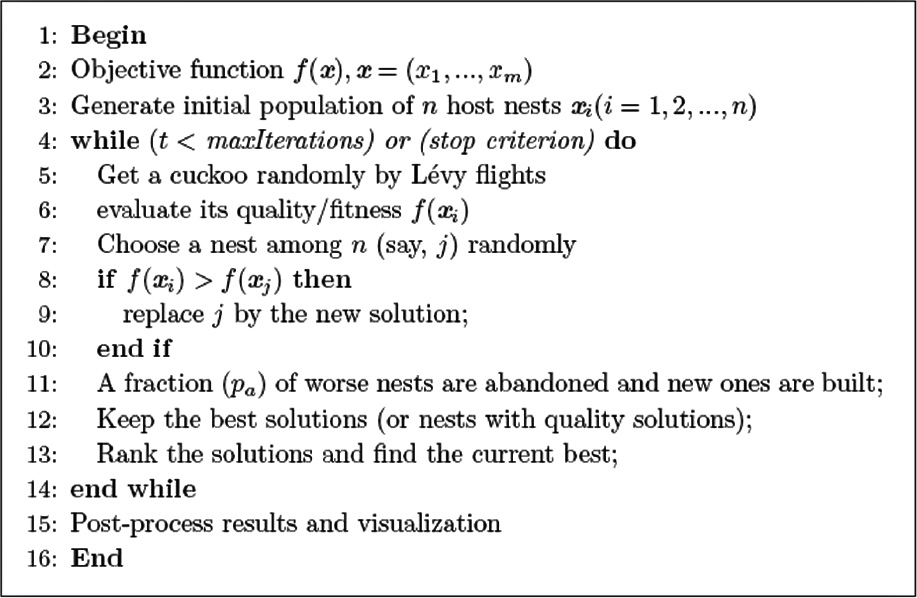
CS Algorithm.

2.4 Initialization of the Algorithm

In CS, the number of host nests is denoted by n. Initially, the solutions in the n nests, denoted by x_i (i=1, 2, …, n), are initialized with random values from the solutions’ range of the objective function f(x). In addition, CS stops when either it reaches a predetermined maximum number of iterations or it satisfies stop criteria based on f(x).

2.5 Update Rule

During each iteration t of CS, a candidate solution (xit) is chosen randomly from the n nests (stored solutions). After that, a new solution (xit+1) is calculated at iteration t+1 by applying a Lévy flight function as follows:

(1)xit+1=xit+α⊕Lévy(λ),

where α>0 is the step value selected based on the size of the tested problem and the symbol ⊕ is the entry-wise product. Exploring the potential solution space using Lévy flight is more efficient than using a random walk because the step length of Lévy flight becomes longer with the progress of the CS algorithm.

The Lévy flight is basically a random walk based on a random step length, which is extracted from a heavy tailed Lévy distribution with an infinite mean and variance [1], given as follows:

(2)Lévy∼u=L−λ,

where L is the step size and λ∈(1, 3) is a parameter related to fractal dimension. It should be noticed that Lévy flight generates a portion of the solutions around the local optima, whereas it generates randomly a significant portion of the solutions away from the local optima. This will allow the CS algorithm to avoid getting stuck around local optima.

3 Hybrid Search Algorithm between CS and SA

In the CS algorithm (Lines 5–10), a cuckoo (solution) i and a nest j are selected randomly. Then, the solution i is replaced by j only when j is better. However, in SA, there is a chance to replace the current solution with a worse successor solution. This process allows SA to avoid getting stuck in a local optima.

Therefore, we adopt this idea from SA to design four variations of CS by hybridizing CS and SA. In all variations (see Figure 4), we replace several steps (Lines 5–10) in the CS algorithm of Figure 3 by calling the SA algorithm to retrieve a cuckoo (solution) as shown in the step (Line 5 in Figure 4). The difference between the four variations is in the arguments passed to the SA algorithm, particularly in the last two arguments. The following summarizes the different calls to SA in the four variations:

In the first variation, SA is called as follows:
x_i ←SIMULATED-ANNEALING(problem, schedule, ∞, LB, UB)
The first two arguments, which are common in the four variations, represent the problem to be solved using the CS algorithm and the scheduling mechanism of the temperature. ∞ means that the number of iterations in SA is independent from the number of iterations of CS. Furthermore, the process of selecting a solution in SA is fully random and should be within the range of the problem (i.e. the lower and upper bounds: LB and UB).
In the second variation, the SA algorithm is called once (represented by the third parameter).
x_i ←SIMULATED-ANNEALING(problem, schedule, 1, LB, UB)
This means that the loop used inside SA iterates for one time. This is because SA is used by CS as a selection method.
In the third variation, maxIterations-t is passed to the SA algorithm as follows:
x_i ←SIMULATED-ANNEALING(problem, schedule, maxIterations-t, LB, UB)
This means that the maximum number of iterations in SA, which depends on the maximum number of iterations (maxIterations) and the number of iterated steps t of CS, decreases in each call to SA.
In the last variation, the range of the search space is passed to SA [i.e. LNeighbors (xit−1) and UNeighbors (xit−1)] as follows:
xit←SIMULATED-ANNEALING(problem, schedule, maxIterations-t, LNeighbors (xit−1), UNeighbors (xit−1)
Intuitively, the range of the search space for the solutions in SA depends on the current best solution of CS and it is calculated by a percentage.

Figure 4:

Hybrid CSA Algorithm.

Figure 5 shows the flow chart of the main steps of the CSA algorithm, which are described as follows:

Step 1: Initialize problem and CSA parameters. In this step, the optimization problem is initially modeled as min(f(x)), where the lower and upper bounds for each decision variable are initialized. Also, the parameters of the CS and SA algorithms are initialized.
Step 2: Generate the initial population of n nests (solutions). For instance, three solutions with 10 decision variables each are shown in Figure 6.
Step 3: In this step, the current population is improved by calling the SA algorithm to enhance a randomly selected solution from the population (e.g. see the modified solutions in Figure 6).
Step 4: Update the population of CSA using the CS procedures (abandon and ranking). In Figure 6, the worst solution (the second one) was selected and replaced by a new solution that is generated randomly.

Figure 5:

Flow Chart of Hybrid CSA Algorithm.

Figure 6:

Numerical Example of CSA.

4 Experiments

4.1 Setup

The performance of the four variations of the proposed hybrid algorithm was compared to the CS and SA algorithms using 10 well-known test functions (Tables 1–8 ). These variations can be distinguished in this section as follows:

CS algorithm,
Variation 1 of the CSA algorithm (CSA1),
Variation 2 of the CSA algorithm (CSA2),
Variation 3 of the CSA algorithm (CSA3),
Variation 4 of the CSA algorithm (CSA4), and
SA algorithm.

Table 1:

Experimental Results of the Algorithms for each of the 10 Benchmark Functions.

Function name	CS	CSA1	CSA2	CSA3	CSA4	SA
Sphere function	2.33E−04	3.31E−10	1.09E−04	5.96E−11	2.12E−10	4.84E−02
	4.16E−04	7.69E−10	3.18E−04	9.65E−11	2.67E−10	1.82E−01
	2.33E−04	3.31E−10	1.09E−04	5.96E−11	2.12E−10	4.84E−02
Easom’s test function	−8.14E−01	−9.95E−01	−7.72E−01	−9.95E−01	−9.96E−01	−7.51E−02
	1.77E−01	1.86E−03	1.63E−01	1.79E−03	6.07E−04	1.97E−01
	1.86E−01	4.78E−03	2.28E−01	5.16E−03	3.63E−03	9.25E−01
Step function	0.00E+00	0.00E+00	0.00E+00	0.00E+00	0.00E+00	5.09E+02
	0.00E+00	0.00E+00	0.00E+00	0.00E+00	0.00E+00	2.77E+03
	0.00E+00	0.00E+00	0.00E+00	0.00E+00	0.00E+00	5.09E+02
Schwefel’s problem	1.28E−03	1.83E−06	6.93E−02	1.27E−06	1.62E−07	4.20E−02
	1.25E−03	1.86E−06	2.00E−01	1.00E−06	1.53E−07	1.57E−01
	1.28E−03	1.83E−06	6.93E−02	1.27E−06	1.62E−07	4.20E−02
Rastrigin’s test function	2.33E−04	3.31E−10	1.09E−04	5.96E−11	2.12E−10	4.84E−02
	4.16E−04	7.69E−10	3.18E−04	9.65E−11	2.67E−10	1.82E−01
	2.33E−04	3.31E−10	1.09E−04	5.96E−11	2.12E−10	4.84E−02
Rotated hyperellipsoid function	4.80E−02	1.52E−07	7.67E−02	7.00E−08	1.14E−09	1.44E+04
	9.77E−02	3.13E−07	2.68E−01	1.31E−07	2.54E−09	3.41E+04
	4.80E−02	1.52E−07	7.67E−02	7.00E−08	1.14E−09	1.44E+04
Beale’s function	3.01E−02	3.03E−02	3.02E−02	3.01E−02	3.03E−02	9.30E−01
	4.60E−04	6.66E−04	5.44E−04	2.88E−04	6.68E−04	2.65E+00
	3.01E−02	3.03E−02	3.02E−02	3.01E−02	3.03E−02	1.16E−04
Shifted sphere function	−4.50E+02	−4.50E+02	−4.50E+02	−4.50E+02	−4.50E+02	1.16E+04
	5.91E−02	1.98E−02	5.29E−02	3.83E−02	5.82E−02	2.77E+03
	7.00E−02	4.42E−03	4.05E−02	3.57E−02	5.00E−02	1.21E+04
Shifted Schwefel’s problem	−4.50E+02	−4.50E+02	−4.50E+02	−4.50E+02	−4.50E+02	3.49E+04
	1.09E−06	2.02E−06	6.59E−07	5.80E−07	3.40E−07	1.38E+04
	6.77E−07	1.11E−06	5.40E−07	4.36E−07	2.53E−07	3.54E+04
Booth’s function	9.69E−03	1.04E−02	7.70E−03	1.05E−02	1.01E−02	1.29E+01
	8.43E−03	9.27E−03	9.84E−03	8.53E−03	8.23E−03	4.68E+00
	9.69E−03	1.04E−02	7.70E−03	1.05E−02	1.01E−02	1.29E+01

The number of decision variables is 10, the number of iterations is 10,000, and the number of runs is 100.

Table 2:

Experimental Results of the Algorithms for each of the 10 Benchmark Functions.

Function name	CS	CSA1	CSA2	CSA3	CSA4	SA
Sphere function	6.04E−07	1.43E−12	2.85E−07	1.37E−12	2.62E−14	2.54E−04
	1.12E−06	2.95E−12	4.59E−07	1.84E−12	4.29E−14	5.91E−04
	6.04E−07	1.43E−12	2.85E−07	1.37E−12	2.62E−14	2.54E−04
Easom’s test function	−8.43E−01	−9.95E−01	−8.09E−01	−9.95E−01	−9.96E−01	−8.29E−02
	1.23E−01	2.22E−03	1.59E−01	1.81E−03	8.81E−04	2.02E−01
	1.57E−01	5.09E−03	1.91E−01	5.27E−03	3.75E−03	9.17E−01
Step function	0.00E+00	0.00E+00	0.00E+00	0.00E+00	0.00E+00	1.16E+01
	0.00E+00	0.00E+00	0.00E+00	0.00E+00	0.00E+00	5.91E+01
	0.00E+00	0.00E+00	0.00E+00	0.00E+00	0.00E+00	1.16E+01
Schwefel’s problem	1.21E−03	1.45E−06	1.91E−02	1.74E−06	1.75E−07	6.46E−02
	1.16E−03	2.05E−06	2.37E−02	1.49E−06	1.35E−07	2.78E−01
	1.21E−03	1.45E−06	1.91E−02	1.74E−06	1.75E−07	6.46E−02
Rastrigin’s test function	7.40E−05	6.76E−10	5.89E−05	2.36E−10	1.44E−10	8.59E−03
	1.09E−04	1.60E−09	8.71E−05	7.13E−10	2.12E−10	1.17E−02
	7.40E−05	6.76E−10	5.89E−05	2.36E−10	1.44E−10	8.59E−03
Rotated hyperellipsoid function	1.15E+00	7.73E−06	1.12E+00	3.71E−08	2.29E+05	1.16E−04
	1.68E+00	1.71E−05	2.00E+00	7.99E−08	1.25E+06	1.16E−04
	1.15E+00	7.73E−06	1.12E+00	3.71E−08	2.29E+05	1.16E−04
Beale’s function	9.92E+14	3.02E−02	3.02E−02	3.00E−02	3.02E−02	9.37E−01
	5.43E+15	5.93E−04	5.36E−04	2.80E−04	5.94E−04	2.64E+00
	9.92E+14	3.02E−02	3.02E−02	3.00E−02	3.02E−02	9.37E−01
Shifted sphere function	1.32E+04	1.23E+03	1.04E+04	−4.45E+02	−4.40E+02	2.16E+04
	1.32E+04	4.09E−04	4.09E−04	4.09E−04	4.09E−04	1.90E+03
	1.37E+04	1.68E+03	1.09E+04	5.00E+00	9.50E+00	2.21E+04
Shifted Schwefel’s problem	−4.50E+02	−4.50E+02	−4.50E+02	−4.50E+02	−4.50E+02	5.59E+05
	5.21E−07	2.11E−06	4.66E−07	6.94E−07	5.77E−07	5.83E+04
	3.50E−07	6.55E−07	3.24E−07	4.12E−07	2.30E−07	5.59E+05
Booth’s function	9.45E−03	1.05E−02	9.99E−03	7.94E−03	9.86E−03	1.46E+01
	7.71E−03	1.01E−02	1.22E−02	8.69E−03	9.94E−03	4.08E+00
	9.45E−03	1.05E−02	9.99E−03	7.94E−03	9.86E−03	1.46E+01

The number of decision variables is 30, the number of iterations is 10,000, and the number of runs is 100.

Table 3:

Experimental Results of the Algorithms for each of the 10 Benchmark Functions.

Function name	CS	CSA1	CSA2	CSA3	CSA4	SA
Sphere function	1.79E−06	1.57E−12	4.01E−07	1.40E−12	1.31E−12	4.00E−03
	4.04E−06	1.68E−12	7.63E−07	2.23E−12	1.96E−12	1.96E−02
	1.79E−06	1.57E−12	4.01E−07	1.40E−12	1.31E−12	4.00E−03
Easom’s test function	−8.24E−01	−9.95E−01	−7.72E−01	−9.95E−01	−9.96E−01	−9.86E−02
	1.77E−01	1.86E−03	1.63E−01	1.79E−03	6.07E−04	2.28E−01
	1.76E−01	4.78E−03	2.28E−01	5.16E−03	3.63E−03	9.01E−01
Step function	0.00E+00	0.00E+00	0.00E+00	0.00E+00	0.00E+00	1.83E+01
	0.00E+00	0.00E+00	0.00E+00	0.00E+00	0.00E+00	7.67E+01
	0.00E+00	0.00E+00	0.00E+00	0.00E+00	0.00E+00	1.83E+01
Schwefel’s problem	1.34E−03	1.66E−06	7.71E−03	1.37E−06	1.63E−07	2.11E−02
	1.36E−03	1.34E−06	6.69E−03	1.31E−06	1.26E−07	6.41E−02
	1.34E−03	1.66E−06	7.71E−03	1.37E−06	1.63E−07	2.11E−02
Rastrigin’s test function	1.66E−04	4.93E−10	1.86E−04	2.46E−10	4.96E−10	1.84E−02
	2.73E−04	6.67E−10	2.53E−04	9.33E−12	3.91E−10	2.08E−02
	1.66E−04	4.93E−10	1.86E−04	2.46E−10	4.96E−10	1.84E−02
Rotated hyperellipsoid function	7.58E+01	5.54E−05	9.66E+01	8.05E−06	2.69E−07	6.80E+03
	1.26E+02	5.54E−05	8.85E+01	2.67E−06	2.19E−07	7.16E+03
	7.58E+01	5.54E−05	9.66E+01	8.05E−06	2.69E−07	6.80E+03
Beale’s function	3.01E−02	3.02E−02	3.02E−02	3.00E−02	3.02E−02	7.87E−01
	3.52E−04	5.93E−04	5.04E−04	2.56E−04	6.49E−04	2.08E+00
	3.01E−02	3.02E−02	3.02E−02	3.00E−02	3.02E−02	7.87E−01
Shifted sphere function	1.32E+05	−4.04E+02	2.31E+04	−4.07E+02	−4.20E+02	1.86E+05
	5.58E+03	1.41E+02	4.99E+04	1.32E+02	1.14E+02	1.04E+04
	1.33E+05	4.63E+01	2.35E+04	4.34E+01	3.00E+01	1.87E+05
Shifted Schwefel’s problem	8.73E+05	4.08E+04	8.47E+05	2.55E+04	5.10E+03	7.91E+06
	2.51E+06	3.48E+03	2.43E+06	2.17E+03	4.35E+02	7.93E+05
	8.74E+05	4.12E+04	8.47E+05	2.59E+04	5.55E+03	7.91E+06
Booth’s function	6.80E−03	1.03E−02	1.02E−02	1.22E−02	1.27E−02	1.35E+01
	7.45E−03	1.14E−02	1.09E−02	1.49E−02	1.23E−02	4.56E+00
	6.80E−03	1.03E−02	1.02E−02	1.22E−02	1.27E−02	1.35E+01

The number of decision variables is 100, the number of iterations is 10,000, and the number of runs is 100.

Table 4:

Experimental Results of the Algorithms for each of the 10 Benchmark Functions.

Function name	CS	CSA1	CSA2	CSA3	CSA4	SA
Sphere function	8.61E−06	1.30E−12	4.49E−07	2.29E−12	2.16E−14	8.90E−05
	4.22E−05	1.96E−12	7.19E−07	3.05E−12	1.97E−14	8.09E−05
	8.61E−06	1.30E−12	4.49E−07	2.29E−12	2.16E−14	8.90E−05
Easom’s test function	−1.43E−01	−9.95E−01	−8.31E−01	−9.93E−01	−9.97E−01	−2.02E−04
	3.28E−01	1.21E−03	2.60E−01	1.73E−03	3.03E−04	2.65E−04
	8.57E−01	4.71E−03	1.69E−01	7.28E−03	3.25E−03	1.00E+00
Step function	0.00E+00	0.00E+00	0.00E+00	0.00E+00	0.00E+00	3.17E+00
	0.00E+00	0.00E+00	0.00E+00	0.00E+00	0.00E+00	3.17E+00
	0.00E+00	0.00E+00	0.00E+00	0.00E+00	0.00E+00	1.83E+01
Schwefel’s problem	1.57E−03	1.76E−06	2.19E−03	1.23E−06	3.20E−07	1.75E−02
	1.35E−03	1.34E−06	1.24E−03	8.12E−07	4.06E−08	1.96E−02
	1.57E−03	1.76E−06	2.19E−03	1.23E−06	3.20E−07	1.75E−02
Rastrigin’s test function	9.90E−04	2.13E−10	4.00E−04	1.73E−10	2.09E−10	2.76E−02
	2.75E−04	1.77E−10	3.13E−04	1.36E−10	1.49E−10	3.81E−02
	9.90E−04	2.13E−10	4.00E−04	1.73E−10	2.09E−10	2.76E−02
Rotated hyperellipsoid function	5.17E+04	4.78E+03	4.53E+04	4.09E+03	2.93E+03	4.79E+07
	4.63E+04	1.02E+04	4.42E+04	7.23E+03	3.65E+03	2.07E+08
	5.17E+04	4.78E+03	4.53E+04	4.09E+03	2.93E+03	4.79E+07
Beale’s function	3.03E−02	3.03E−02	3.01E−02	3.03E−02	3.01E−02	2.68E−01
	6.51E−04	4.78E−04	4.43E−04	5.69E−04	2.73E−04	4.91E−02
	3.03E−02	1.16E−04	3.01E−02	3.03E−02	3.01E−02	2.68E−01
Shifted sphere function	1.32E+05	1.19E+03	9.23E+04	1.12E+03	1.15E+03	2.15E+06
	6.00E+03	5.40E+01	4.20E+03	5.11E+01	5.21E+01	5.77E+05
	1.32E+05	1.64E+03	9.28E+04	1.57E+03	1.60E+03	2.15E+06
Shifted Schwefel’s problem	5.88E+06	7.23E+05	5.39E+06	5.53E+05	6.95E+04	1.01E+09
	1.81E+06	2.22E+05	1.66E+06	1.70E+05	2.14E+04	1.95E+06
	5.88E+06	7.24E+05	5.39E+06	5.54E+05	7.00E+04	1.01E+09
Booth’s function	6.64E−03	1.13E−02	9.33E−03	1.24E−02	1.37E−02	1.40E+01
	6.89E−03	1.19E−02	1.10E−02	1.44E−02	1.27E−02	3.97E+00
	6.64E−03	1.13E−02	9.33E−03	1.24E−02	1.37E−02	1.40E+01

The number of decision variables is 1000, the number of iterations is 10,000, and the number of runs is 100.

Table 5:

Convergence Results of the Algorithms for each of the 10 Benchmark Functions.

Function name	CS	CSA1	CSA2	CSA3	CSA4	SA
Sphere function	2.13E+04	6.05E+02	1.00E+04	6.78E+02	1.28E+02	*
	2.89E+03	5.02E+02	0.00E+00	5.13E+02	1.33E+02	*
Easom’s test function	7.02E+03	8.16E+01	4.64E+03	1.12E+02	8.14E+01	9.17E+02
	4.36E+03	1.00E+02	4.57E+03	8.64E+01	3.85E+01	0.00E+00
Step function	2.22E+02	1.37E+00	1.79E+02	1.40E+00	1.50E+00	5.20E+02
	2.25E+02	6.15E−01	1.47E+02	7.70E−01	8.20E−01	3.28E+01
Schwefel’s problem	9.14E+03	1.42E+01	1.38E+01	1.80E+01	2.60E+00	*
	1.91E+03	1.44E+01	1.16E+01	1.87E+01	1.52E+00	*
Rastrigin’s test function	1.00E+04	2.39E+03	1.00E+04	1.41E+03	2.83E+03	*
	0.00E+00	7.71E+02	0.00E+00	5.51E+01	2.68E+03	*
Rotated hyperellipsoid function	1.00E+04	2.67E+03	6.67E+03	4.37E+03	8.47E+01	*
	0.00E+00	3.78E+03	5.77E+03	5.12E+03	8.16E+01	*
Beale’s function	1.00E+04	9.56E+03	4.38E+03	4.45E+03	8.98E+03	*
	0.00E+00	1.90E+03	3.51E+03	4.90E+03	1.77E+03	*
Shifted sphere function	1.62E+05	6.90E+04	1.52E+05	6.64E+04	6.37E+04	*
	3.29E+04	2.36E+04	4.51E+04	2.28E+04	2.18E+04	*
Shifted Schwefel’s problem	1.41E+04	2.87E+03	1.35E+04	6.71E+03	2.94E+03	*
	2.35E+03	3.50E+03	2.25E+03	2.23E+03	3.03E+03	*
Booth’s function	7.02E+03	8.16E+01	4.40E+03	1.12E+02	8.14E+01	6.32E+03
	4.36E+03	1.00E+02	4.27E+03	8.64E+01	3.85E+01	4.39E+03

Table 6:

Comparison of the Running Time of all the Variations of CSA to the Running Time of CS and SA.

Function name	CS	CSA1	CSA2	CSA3	CSA4	SA
Sphere function	1.20E+03	1.05E+04	1.11E+03	1.19E+04	1.20E+04	1.60E+01
Easom’s test function	9.68E+02	2.44E+04	7.96E+02	2.88E+04	3.15E+04	1.50E+01
Step function	1.22E+03	4.63E+04	1.40E+03	6.06E+04	5.99E+04	2.80E+01
Schwefel’s problem	6.47E+02	1.65E+04	1.50E+01	1.93E+04	2.01E+04	1.20E+01
Rastrigin’s test function	1.74E+03	2.99E+05	2.72E+03	3.51E+05	3.52E+05	1.89E+02
Rotated hyperellipsoid function	1.02E+03	9.10E+03	7.51E+02	1.01E+04	9.55E+03	1.60E+01
Beale’s function	9.08E+02	3.56E+03	7.04E+02	4.42E+03	4.05E+03	2.00E+00
Shifted sphere function	1.21E+04	3.52E+06	1.81E+04	3.81E+06	3.21E+06	1.44E+04
Shifted Schwefel’s problem	1.05E+03	3.23E+05	1.68E+03	3.66E+05	3.66E+05	4.70E+01
Booth’s function	1.11E+03	3.48E+03	6.24E+02	3.84E+03	3.57E+03	1.20E+01

The number of decision variables is 100, the number of iterations is 10,000, and the number of runs is 100.

Table 7:

Comparison of the Running Time of all the Variations of CSA to the Running Time of CS and SA based on the Convergence to the Best Value of CS.

Function name	CS	CSA1	CSA2	CSA3	CSA4	SA
Sphere function	1.29E+03	1.70E+01	7.36E+02	2.80E+01	9.00E+00	5.43E+03
Easom’s test function	9.05E+02	4.70E+01	1.50E+01	1.25E+02	7.80E+01	9.56E+02
Step function	1.14E+03	1.60E+01	1.40E+01	3.10E+01	3.20E+01	1.12E+04
Schwefel’s problem	7.95E+02	6.70E+01	3.00E+01	1.00E+02	1.00E+01	5.10E+01
Rastrigin’s test function	1.89E+03	1.73E+02	1.48E+03	3.12E+02	2.51E+02	2.73E+03
Rotated hyperellipsoid function	8.02E+02	5.52E+02	1.20E+03	7.11E+02	1.85E+02	1.51E+02
Beale’s function	1.27E+03	3.68E+03	1.16E+03	3.92E+03	4.21E+03	9.00E+00
Shifted sphere function	3.30E+01	1.40E+01	2.00E+00	1.80E+01	1.90E+01	8.20E+01
Shifted Schwefel’s problem	1.02E+03	3.25E+05	1.04E+04	3.24E+05	3.11E+05	*
Booth’s function	8.10E+02	3.47E+03	1.15E+03	6.81E+02	3.53E+03	1.92E+04

Table 8:

Comparison of the Running Time of all the Variations of CSA to the Running Time of CS and SA based on the Convergence to the Best Value of CSA4.

Function name	CS	CSA1	CSA2	CSA3	CSA4	SA
Sphere function	1.52E+03	7.50E+01	6.87E+02	7.80E+01	3.30E+01	2.52E+03
Easom’s test function	2.22E+02	2.10E+01	3.00E+00	1.02E+02	3.32E+02	9.39E+02
Step function	1.12E+03	5.10E+01	5.60E+01	3.30E+01	2.90E+01	3.13E+03
Schwefel’s problem	1.40E+04	1.65E+04	2.18E+04	1.92E+04	1.94E+04	9.00E+04
Rastrigin’s test function	*	2.21E+05	*	1.45E+05	1.33E+05	*
Rotated hyperellipsoid function	*	2.61E+02	2.22E+05	6.93E+03	1.20E+01	*
Beale’s function	*	4.02E+03	*	4.66E+03	3.03E+03	*
Shifted sphere function	*	8.17E+04	*	6.12E+04	3.38E+04	*
Shifted Schwefel’s problem	*	7.34E+05	*	5.86E+05	4.58E+05	*
Booth’s function	1.79E+03	2.81E+03	7.85E+02	1.69E+03	3.87E+03	*

All the variations of CSA used the same parameter settings as suggested by Yang and Deb [30]: the population size n=15, the step size of the Lévy flight β=1, and the fraction of abandon nests P_a=0.25. For the SA algorithm, the temperature T=1000 and the cooling rate c=0.01.

In all experiments, each algorithm was executed 100 times as recommended by Yang and Deb [29], [30], [31] for similar optimization problems to provide meaningful statistical analysis of the proposed variations of CS. For CSA4, the range of the search space (Line 5 in Figure 4) is 15% below and above the current best solution.

The experiments were conducted using an Intel Core i7-4510U, 1.8 GHz CPU with 16 GB RAM running 64-bit Windows. All the algorithms were implemented using Java programming language. Table 9 provides a summary of the benchmark functions, which have been used for evaluating CS algorithm as well as other famous optimization algorithms [30], [31]. The dimensions for the benchmark functions are as follows:

2 for Easom’s, Beale’s, and Booth’s test functions and
10, 30, 100, and 1000 for the rest of the functions.

Table 9:

Benchmark Functions used to Evaluate the Algorithms.

Function name	Expression	Search range	Optimum value	Category [22]
Sphere function [21]	f1(x)=∑i=1Nxi2	x_i ∈[−100,100]	min(f₁)=f(0, …, 0)=0	Unimodal
Easom’s test function	f₂(x, y)–cos(x)cos(y)exp[–(x–π)² –(y–π)²]	(x, y)∈[−100,100] ×[−100,100]	min(f₂)=f(π, π)=−1	Unimodal
Step function [21]	f3(x)=∑i=1N(⌊xi+0.5⌋)2	x_i ∈[−100,100]	min(f₃)=f(0, …, 0)=0	Discontinuous unimodal
Schwefel’s problem 2.22	f4(x)=−∑i=1N(xi)+∏i=1N(xi)	x_i ∈[−10,10]	min(f₄)=f(0, …, 0)=0	Unimodal
Rastrigin’s test function [27]	f5(x)=∑i=1N(xi2−10cos(2πxi)+10)	x_i ∈[−5.12,5.12]	min(f₅)=f(0, …, 0)=0	Multimodal
Rotated hyperellipsoid function	f6(x)=∑i=1N(∑j=1ixj)2	x_i ∈[−100,100]	min(f₆)=f(0, …, 0)=0	Unimodal
Beale’s function	f₇(x, y)=(1.5–x+xy)²+(2.25–x+xy²)²+(2.625–x+xy³)²	x, y∈[−4.5,4.5]	min(f₇)=f(3, 0.5)=0	Multimodal
Shifted sphere function [27]	f8(x)=∑i=1Nzi2+f_bias1, where z=x–o	x_i ∈[−100,100]	min(f₈)=f(o₁, …, o_N) =f_bias₁=−450	Unimodal
Shifted Schwefel’s problem 1.2 [27]	f9(x)=∑i=1N(∑j=1izj)2+f_bias2, where z=x-o	x_i ∈[−100,100]	min(f₉)=f(o₁, …, _oN) =f_bias₂=−450	Unimodal
Booth’s function	f₁₀(x, y)=(x+2y–7)²+(2x+y–5)²	x, y∈[−10,10]	min(f₁₀)=f(1, 3)=0	Unimodal

4.2 Comparison of CS, SA, and the Proposed Four Variations of CSA: Results and Discussion

Tables 1–4 report the experimental results with respect to each of the 10 benchmark functions described in Table 9. The results are in the following format: average of 100 independent runs (row 1), standard deviation (row 2), and error value (row 3) for the best solutions. The error value is the distance from the global minimal solution to the average of the best solutions [6].

The main goal of the experiments is to compare the performance of the proposed variations of CSA to the performance of CS and SA. For the 10D functions shown in Table 1, all the variations of CSA (CSA1–CSA4) perform better than the CS and SA algorithms. It can also be noted that CSA4 outperforms all the other algorithms for 4 of 10 test functions. However, the results of CSA3 are less but near to the results of CSA4 for most of the test functions. On the contrary, the CSA2 variation provides minor enhancement to the performance of the original CS algorithm. This could be justified by the fact that CSA2 does not deeply search for better solutions within the whole range of potential solutions like the other variations of CSA. In other words, CSA2 uses the SA algorithm as a selection method but not as an exploration algorithm.

Table 2 shows the results of the 30D test functions. The CSA4 and CSA3 variations again outperform all the other algorithms for 5 of 10 functions and 4 of 10 functions, respectively. In addition, the CSA2 algorithm performs slightly better than the CS and SA algorithms. However, the other variations of CSA perform much better than CSA2. These observations confirm the observations obtained from Table 1.

As in Tables 1 and 2, the reported results in Table 3 for the 100D problems indicate that all the variations of CSA outperform the CS and SA algorithms. Obviously, CSA4 is the best performing algorithm (superior performance for 6 of 10 functions) and CSA2 is the worst performing variation of CSA. The same observations noted in Tables 1–3 apply to Table 4 (functions with 1000D).

To sum up, the overall results of the experiments indicate that all the variations of CSA perform better than the CS and SA algorithms. In general, CSA4 is the most efficient variation of CSA, whereas CSA2 is the least efficient variation of CSA. This might be because CSA4 performs a local search within the neighbors of the current solutions, whereas CSA2 performs a shallow search for better solutions. In addition, all the population-based search algorithms perform better than SA (single-solution search algorithm).

Table 5 summarizes the convergence results of the tested algorithms using the 10 test functions with dimension 10. The results are in the following format: average number (row 1) and standard deviation of iterations (row 2). The number of iterations for each algorithm is reported in Table 5 when the variations of the values of the test function is less than a given threshold value ε≤10⁻¹⁰. As shown in Table 5, all the variations of CSA perform much better than CS and SA. In other words, all the variations of CSA converge faster to solutions than CS and SA. In addition, CSA3 and CSA4 are the fastest converging algorithms, whereas SA is the slowest converging algorithm.

4.3 Runtime Performance Comparison of CS, SA, and the Proposed Four Variations of CSA

Tables 6–8 provide the running time comparison of CS, SA, and the proposed four variations of CSA for each of the 10 benchmark functions described in Table 9 (the number of decision variables is 100). The results are reported in milliseconds representing the average of 100 independent runs.

The values in Table 6 for each algorithm was reported after 10,000 iterations, which represent the running time required to obtain the results in Table 3. As shown in the table, SA followed by CS are faster than the other algorithms. However, SA and CS do not provide better objective values compared to the other algorithms (as shown in Table 3 for the same dimension).

Table 7 shows the running time of all the variations of CSA as well as CS and SA, which were reported when each algorithm converged to the best objective value of CS (see Table 3). In the same way, Table 8 shows the running time of all the variations of CSA as well as CS and SA, which were reported when each algorithm converged to the best objective value of CSA4 (see Table 3).

As shown in Table 7, all the proposed variations converge to the target solution faster than CS and SA for all functions (except one). Also, as shown in Table 8, all the proposed variations (except CSA2) converge to the target solution faster than CS and SA for all functions (except one). It should be noticed that some algorithms did not converge to the target solution, denoted by *, for some functions within reasonable time.

4.4 Comparison of CSA3, CSA4, and Other Well-Known Optimization Algorithms

The performance of the two most successful variations of CSA according to Tables 1–8 was compared to the performance of particle swarm optimization (PSO) algorithm [3], Bat algorithm (BA) [1], [32], Boltzman CS algorithm (BCS), and ε-greedy CS algorithm (EGCS) [2] as shown in Tables 10 and 11. The parameters of the algorithms in Tables 10 and 11 were set as follows:

As recommended by Abed-alguni et al. [1], [3], the weight parameters in PSO were W=0, C1=C2=1.
For the BA algorithm, the discount parameter of the frequencies β=0.5, the loudness A=1, and the pulse rate r=0 for each candidate solution.
For EGCS, the exploration parameter ε =0.1 as suggested by Abed-alguni and Alkhateeb [2].
For BCS, the temperature T=0.1 as suggested by Abed-alguni and Alkhateeb [2].

Table 10:

Comparison Results of CSA3 and CSA4 to Four Other Optimization Algorithms.

Function name	CSA3	CSA4	BA	BCS	EGCS	PSO
Sphere function	1.19E−12	2.00E−14	1.30E−07	2.24E−07	4.73E−07	1.47E−06
	1.85E−12	3.07E−14	1.49E−07	4.19E−07	9.60E−07	3.54E−06
	1.19E−12	2.00E−14	1.30E−07	2.24E−07	4.73E−07	1.47E−06
Easom’s test function	−9.95E−01	−9.96E−01	−9.82E−50	−8.86E−01	−8.47E−01	−4.19E−12
	1.96E−03	3.56E−03	3.26E−49	8.97E−02	1.15E−01	2.30E−11
	5.19E−03	4.30E−03	1.00E+00	1.14E−01	1.53E−01	1.00E+00
Step function	0.00E+00	0.00E+00	0.00E+00	0.00E+00	0.00E+00	0.00E+00
	0.00E+00	0.00E+00	0.00E+00	0.00E+00	0.00E+00	0.00E+00
	0.00E+00	0.00E+00	0.00E+00	0.00E+00	0.00E+00	0.00E+00
Schwefel’s problem	1.39E−06	1.49E−07	0.00E+00	6.63E−04	0.00E+00	2.25E−03
	1.42E−06	1.22E−07	0.00E+00	4.41E−04	0.00E+00	3.06E−03
	1.39E−06	1.49E−07	0.00E+00	6.63E−04	0.00E+00	2.25E−03
Rastrigin’s test function	8.58E−11	1.24E−10	2.52E−05	2.28E−05	1.99E−05	1.19E−04
	1.34E−10	2.09E−10	2.99E−05	3.79E−05	2.44E−05	2.90E−04
	8.58E−11	1.24E−10	2.52E−05	2.28E−05	1.99E−05	1.19E−04
Rotated hyperellipsoid function	3.00E−02	3.02E−02	9.93E−01	2.16E−05	2.01E−05	3.12E+00
	2.68E−04	6.14E−04	1.55E+00	3.72E−05	2.38E−05	8.89E+00
	3.00E−02	3.02E−02	9.93E−01	2.16E−05	2.01E−05	3.12E+00
Beale’s function	3.00E−02	3.02E−02	8.35E−02	3.02E−02	3.03E−02	3.02E−02
	2.68E−04	6.14E−04	2.07E−01	4.03E−04	6.07E−04	5.87E−04
	3.00E−02	3.02E−02	8.35E−02	3.02E−02	3.03E−02	3.02E−02
Shifted sphere function	−4.45E+02	−4.40E+02	1.99E+04	2.20E+04	2.24E+04	1.96E+04
	2.74E+01	3.65E+01	7.12E+03	1.78E+03	1.64E+03	8.16E+03
	5.00E+00	9.50E+00	2.04E+04	2.24E+04	2.29E+04	2.01E+04
Shifted Schwefel’s problem	−4.50E+02	−4.50E+02	−4.50E+02	−4.50E+02	−4.50E+02	−4.50E+02
	1.03E−05	1.02E−05	2.25E−01	6.34E−07	3.46E−07	2.11E−05
	2.28E−06	2.07E−06	5.63E−02	3.39E−07	2.49E−07	4.17E−06
Booth’s function	7.94E−03	9.86E−03	2.20E−02	6.34E−03	1.26E−02	1.49E−02
	8.69E−03	9.94E−03	4.38E−02	6.44E−03	1.35E−02	2.72E−02
	7.94E−03	9.86E−03	2.20E−02	6.34E−03	1.26E−02	1.49E−02

The number of decision variables is 30, the number of iterations is 10,000, and the number of runs is 100.

Table 11:

Comparison Results of CSA3 and CSA4 to Four Other Optimization Algorithms.

Function name	CSA3	CSA4	BA	BCS	EGCS	PSO
Sphere function	1.40E−12	1.31E−12	3.21E−07	4.13E−07	3.70E−07	1.12E−05
	2.23E−12	1.96E−12	4.27E−07	8.03E−07	8.34E−07	3.41E−05
	1.40E−12	1.31E−12	3.21E−07	4.13E−07	3.70E−07	1.12E−05
Easom’s test function	−9.95E−01	−9.96E−01	−1.56E−32	−8.47E−01	−7.81E−01	1.91E−22
	1.79E−03	6.07E−04	5.94E−32	9.20E−02	2.00E−01	6.34E−22
	5.16E−03	3.63E−03	1.00E+00	1.53E−01	2.19E−01	1.00E+00
Step function	0.00E+00	0.00E+00	0.00E+00	0.00E+00	0.00E+00	0.00E+00
	0.00E+00	0.00E+00	0.00E+00	0.00E+00	0.00E+00	0.00E+00
	0.00E+00	0.00E+00	0.00E+00	0.00E+00	0.00E+00	0.00E+00
Schwefel’s problem	1.37E−06	1.63E−07	7.26E−04	4.92E−04	0.00E+00	2.18E−03
	1.31E−06	1.26E−07	5.52E−04	3.91E−04	0.00E+00	4.47E−03
	1.37E−06	1.63E−07	7.26E−04	4.92E−04	0.00E+00	2.18E−03
Rastrigin’s test function	2.46E−10	4.96E−10	5.37E−05	8.71E−05	3.15E−05	6.72E−04
	9.33E−12	3.91E−10	1.21E−04	1.89E−04	8.35E−05	1.54E−03
	2.46E−10	4.96E−10	5.37E−05	8.71E−05	3.15E−05	6.72E−04
Rotated hyperellipsoid function	8.05E−06	2.69E−07	2.64E+01	1.79E+01	7.75E+01	3.12E+01
	2.67E−06	2.19E−07	3.19E+01	2.45E+01	1.63E+02	3.08E+01
	8.05E−06	2.69E−07	2.64E+01	1.79E+01	7.75E+01	3.12E+01
Beale’s function	3.00E−02	2.95E−02	3.21E−02	3.22E−02	3.47E−02	8.44E−02
	2.56E−04	3.69E−03	1.09E−02	7.93E−03	9.09E−03	1.15E−01
	3.00E−02	2.95E−02	3.21E−02	3.22E−02	3.47E−02	8.44E−02
Shifted sphere function	−4.07E+02	−4.20E+02	1.45E+05	1.36E+05	1.38E+05	1.36E+05
	1.32E+02	1.14E+02	1.74E+04	6.49E+03	6.06E+03	8.51E+03
	4.34E+01	3.00E+01	1.45E+05	1.37E+05	1.38E+05	1.36E+05
Shifted Schwefel’s problem	2.55E+04	5.10E+03	5.26E+06	5.36E+06	5.52E+06	6.84E+06
	2.17E+03	4.35E+02	6.21E+05	7.53E+05	1.32E+06	1.70E+06
	2.59E+04	5.55E+03	5.26E+06	5.36E+06	5.52E+06	6.84E+06
Booth’s function	1.22E−02	1.27E−02	1.18E−02	5.63E−03	7.46E−03	4.36E−02
	1.49E−02	1.23E−02	1.04E−02	6.06E−03	6.37E−03	1.31E−01
	1.22E−02	1.27E−02	1.18E−02	5.63E−03	7.46E−03	4.36E−02

The number of decision variables is 100, the number of iterations is 10,000, and the number of runs is 100.

Tables 10 and 11 show the experimental results with respect to each of the 10 benchmark functions described in Table 9. The average of 100 independent runs (row 1), standard deviation (row 2), and error value (row 3) for the best solutions are shown in the tables.

For the 30D functions shown in Table 10, CSA3 and CSA4 outperform the other algorithms for 5 of 10 test functions. Moreover, as we scale the problem dimensionality from 30D to 100D, CSA3 and CSA4 perform even better (7 of 10 functions). This indicates that the performance of CSA3 and CSA4 improves as the problem complexity increases compared to the other algorithms.

5 Conclusion

The CS and SA algorithms have been successfully used for optimizing both discrete and continuous optimization problems. However, these algorithms do not converge to good solutions when applied to complex optimization problems as shown in the current paper.

This paper presented four novel variations of a hybrid CS and SA algorithm that increases the chance of avoiding local optima. More precisely, these variations use the SA algorithm to provide a chance for exploring the solution space by replacing current solutions by worse ones with a decreasing probability. In other words, unlike CS, CSA overcomes the problem of premature convergence using SA and its operators.

The four variations of CSA as well as CS and SA were compared using well-known benchmark functions. The dimensions for the benchmark functions are 2, 10, 30, 100, and 1000. The experimental results show that three variations of the hybrid algorithm in all of the tested functions (with dimensions of 2, 10, 30, 100, and 1000) provide major improvement of the performance of CS and SA, whereas one variation provides minor improvement. However, for the two-dimensional test functions, all algorithms provide slightly similar performance results.

In addition, the experiments show that the proposed variations of the hybrid algorithm provide better objective values and comparable (sometimes better) computational time compared to CS and SA.

Finally, the performance of the two most successful variations of CSA (namely, CSA3 and CSA4) was compared to the performance of PSO algorithm, BA, BCS, and EGCS. As shown in the experiments, the performance of CSA3 and CSA4 improves as the problem complexity increases compared to the above-mentioned algorithms. Also, these results suggest that the variations of CSA (in particular, CSA3 and CSA4) can be used for solving simple and complex problems.

Bibliography

[1] B. H. Abed-alguni, Bat q-learning algorithm, Jord. J. Comput. Inf. Technol.3 (2017), 56–77.Search in Google Scholar

[2] B. H. Abed-alguni and F. Alkhateeb, Novel selection schemes for cuckoo search, Arab. J. Sci. Eng.42 (2017), 3635–3654.10.1007/s13369-017-2663-3Search in Google Scholar

[3] B. H. Abed-Alguni, D. J. Paul, S. K. Chalup and F. A. Henskens, A comparison study of cooperative q-learning algorithms for independent learners, Int. J. Artif. Intell.14 (2016), 71–93.Search in Google Scholar

[4] V. Černý, Thermodynamical approach to the traveling salesman problem: an efficient simulation algorithm, J. Optim. Theory Appl.45 (1985), 41–51.10.1007/BF00940812Search in Google Scholar

[5] Y. Feng, G.-G. Wang and X.-Z. Gao, A novel hybrid cuckoo search algorithm with global harmony search for 0-1 knapsack problems, Int. J. Comput. Intell. Syst.9 (2016), 1174–1190.10.1080/18756891.2016.1256577Search in Google Scholar

[6] B. H. F. Hasan, I. A. Doush, E. Al Maghayreh, F. Alkhateeb and M. Hamdan, Hybridizing harmony search algorithm with different mutation operators for continuous problems, Appl. Math. Comput.232 (2014), 1166–1182.10.1016/j.amc.2013.12.139Search in Google Scholar

[7] K. Huang, Y. Zhou, X. Wu and Q. Luo, A cuckoo search algorithm with elite opposition-based strategy, J. Intell. Syst.25 (2016), 567–593.10.1515/jisys-2015-0041Search in Google Scholar

[8] W. Kartous, A. Layeb and S. Chikhi, A new quantum cuckoo search algorithm for multiple sequence alignment, J. Intell. Syst.23 (2014), 261–275.10.1515/jisys-2013-0052Search in Google Scholar

[9] A. Khachaturyan, S. Semenovskaya and B. Vainstein, A statistical-thermodynamic approach to determination of structure amplitude phases, Sov. Phys. Crystallogr.24 (1979), 519–524.Search in Google Scholar

[10] S. Kirkpatrick, C. D. Gelatt and M. P. Vecchi, Optimization by simulated annealing, Science220 (1983), 671–680.10.1126/science.220.4598.671Search in Google Scholar PubMed

[11] Q. Liao, S. Zhou, H. Shi and W. Shi, Parameter estimation of nonlinear systems by dynamic cuckoo search, Neural Comput.29 (2017), 1103–1123.10.1162/NECO_a_00946Search in Google Scholar PubMed

[12] A. Lim, B. Rodrigues and X. Zhang, A simulated annealing and hill-climbing algorithm for the traveling tournament problem, Eur. J. Oper. Res.174 (2006), 1459–1478.10.1016/j.ejor.2005.02.065Search in Google Scholar

[13] C. Liu and J. Wang, Cell formation and task scheduling considering multi-functional resource and part movement using hybrid simulated annealing, Int. J. Comput. Intell. Syst.9 (2016), 765–777.10.1080/18756891.2016.1204123Search in Google Scholar

[14] M. Lundy, Applications of the annealing algorithm to combinatorial problems in statistics, Biometrika72 (1985), 191–198.10.1093/biomet/72.1.191Search in Google Scholar

[15] M. Marichelvam, An improved hybrid cuckoo search (IHCS) metaheuristics algorithm for permutation flow shop scheduling problems, Int. J. Bio-Inspired Comput.4 (2012), 200–205.10.1504/IJBIC.2012.048061Search in Google Scholar

[16] M. Marichelvam and M. Geetha, A hybrid cuckoo search metaheuristic algorithm for solving single machine total weighted tardiness scheduling problems with sequence dependent setup times, Int. J. Comput. Complex. Intell. Algorithms1 (2016), 23–34.10.1504/IJCCIA.2016.077463Search in Google Scholar

[17] M. Marichelvam and Ö. Tosun, Performance comparison of cuckoo search algorithm to solve the hybrid flow shop scheduling benchmark problems with makespan criterion. Int. J. Swarm Intell. Res.7 (2016), 1–14.10.4018/IJSIR.2016040101Search in Google Scholar

[18] M. Marichelvam, T. Prabaharan and X.-S. Yang, Improved cuckoo search algorithm for hybrid flow shop scheduling problems to minimize makespan, Appl. Soft Comput.19 (2014), 93–101.10.1016/j.asoc.2014.02.005Search in Google Scholar

[19] U. Mlakar and I. Fister, Hybrid self-adaptive cuckoo search for global optimization, Swarm Evol. Comput.29 (2016), 47–72.10.1016/j.swevo.2016.03.001Search in Google Scholar

[20] P. Mohapatra, S. Chakravarty and P. Dash, An improved cuckoo search based extreme learning machine for medical data classification, Swarm Evol. Comput.24 (2015), 25–49.10.1016/j.swevo.2015.05.003Search in Google Scholar

[21] M. G. H. Omran and M. Mahdavi, Global-best harmony search, Appl. Math. Comput.198 (2008), 643–656.10.1016/j.amc.2007.09.004Search in Google Scholar

[22] Q.-K. Pan, P. N. Suganthan, M. F. Tasgetiren and J. J. Liang, A self-adaptive global best harmony search algorithm for continuous optimization problems, Appl. Math. Comput.216 (2010), 830–848.10.1016/j.amc.2010.01.088Search in Google Scholar

[23] H. Rakhshani and A. Rahati, Intelligent multiple search strategy cuckoo algorithm for numerical and engineering optimization problems, Arab. J. Sci. Eng.42 (2017), 567. https://doi.org/10.1007/s13369-016-2270-8.10.1007/s13369-016-2270-8Search in Google Scholar

[24] Z. Sheng, J. Wang, S. Zhou and B. Zhou, Parameter estimation for chaotic systems using a hybrid adaptive cuckoo search with simulated annealing algorithm, Chaos24 (2014), 013133.10.1063/1.4867989Search in Google Scholar

[25] N. Shivasankaran, P. S. Kumar, G. Nallakumarasamy and K. V. Raja, Repair shop job scheduling with parallel operators and multiple constraints using simulated annealing, Int. J. Comput. Intell. Syst.6 (2013), 223–233.10.1080/18756891.2013.768434Search in Google Scholar

[26] N. Shivasankaran, P. S. Kumar and K. V. Raja, Hybrid sorting immune simulated annealing algorithm for flexible job shop scheduling, Int. J. Comput. Intell. Syst.8 (2015), 455–466.10.1080/18756891.2015.1017383Search in Google Scholar

[27] P. N. Suganthan, N. Hansen, J. J. Liang, K. Deb, Y.-P. Chen, A. Auger and S. Tiwari, Problem definitions and evaluation criteria for the CEC 2005 special session on real-parameter optimization. Technical Report KanGAL Report#2005005, IIT Kanpur, India, Nanyang Technological University, Singapore, 2005.Search in Google Scholar

[28] H. Szu and R. Hartley, Fast simulated annealing, Phys. Lett. A122 (1987), 157–162.10.1016/0375-9601(87)90796-1Search in Google Scholar

[29] X.-S. Yang, Bat algorithm and cuckoo search: a tutorial, in: Artificial Intelligence, Evolutionary Computing and Metaheuristics, pp. 421–434, Springer, 2013.10.1007/978-3-642-29694-9_17Search in Google Scholar

[30] X.-S. Yang and S. Deb, Cuckoo search via Lévy flights, in: World Congress on Nature & Biologically Inspired Computing, 2009, NaBIC 2009, pp. 210–214, IEEE, 2009.10.1109/NABIC.2009.5393690Search in Google Scholar

[31] X.-S. Yang and S. Deb, Engineering optimisation by cuckoo search, Int. J. Math. Modell. Numer. Optim.1 (2010), 330–343.10.1504/IJMMNO.2010.035430Search in Google Scholar

[32] X.-S. Yang and A. Hossein Gandomi, Bat algorithm: a novel approach for global engineering optimization, Eng. Comput.29 (2012), 464–483.10.1108/02644401211235834Search in Google Scholar

[33] Y.-R. Zeng, L. Peng, J. Zhang and L. Wang, An effective hybrid differential evolution algorithm incorporating simulated annealing for joint replenishment and delivery problem with trade credit, Int. J. Comput. Intell. Syst.9 (2016), 1001–1015.10.1080/18756891.2016.1256567Search in Google Scholar

Received: 2017-06-05

Published Online: 2017-10-05

Published in Print: 2019-09-25

This article is distributed under the terms of the Creative Commons Attribution Non-Commercial License, which permits unrestricted non-commercial use, distribution, and reproduction in any medium, provided the original work is properly cited.

Articles in the same Issue

https://doi.org/10.1515/jisys-2017-0268

Keywords for this article

Cuckoo search; simulated annealing search; optimization; metaheuristic

Creative Commons

BY-NC-ND 3.0