Matching estimators of causal effects in clustered observational studies

1 Introduction

2 MPA data and exploratory analysis

The MPA dataset created by Gill et al. [6] includes social, environmental, and ecological information in 9987 sites within 215 MPAs worldwide (Figure 1). The number of sites in each MPA ranges from 1 to 1619, with a mean of 46 and a median of 8. Among 9987 sites, 3988 sites receive the NT policy, whereas 5999 are under the MU policy. The outcome variable is total fish biomass at each site, recorded in underwater visual surveys. There are 13 continuous covariates and 4 categorical covariates that describe the MPA-level and site-level features (Table 1). MPA-level covariates include MPA size and country. The other covariates include site-level social and environmental conditions, as well as sampling protocol, location, and date.

Figure 1

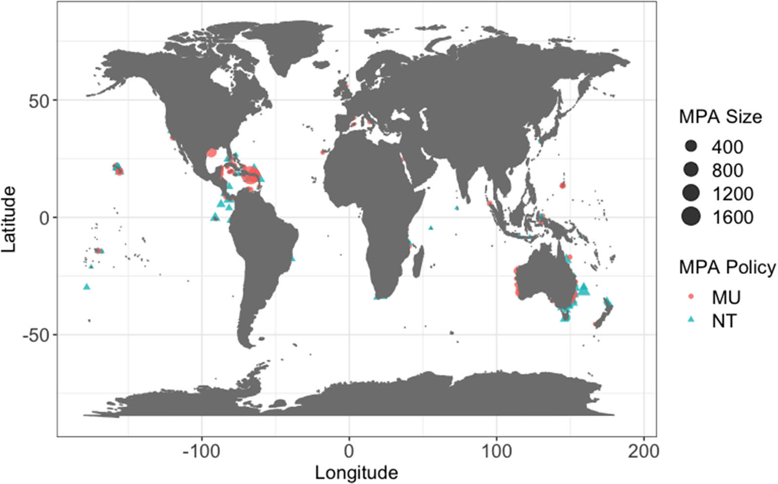
Map showing MPA location, size and policy type (MU = multi-use, NT = no-take); MPA policies are present by the majority within each MPA.

Sites within the same MPA usually receive the same policy (i.e., same fishing regulations), and each site belongs only to one MPA. As a result, the dataset is naturally clustered where observed sites are nested within the MPA, and conservation policies are geographically clustered. The cluster structure brings difficulty in causal inference due to potential confounding. Both cluster-level and site-level covariates could contribute to the confounding bias. Sites in the same MPA share common environmental, MPA-level, and geographical characteristics, affecting both the fish population and MPA policy assignment [3,6,21]. Site-specific covariates, including depth, distance to population centers (also called “markets”), size of neighboring human population, and chlorophyll concentration, are also relevant to the ecological outcome [6,22–24]. Within the same MPA, implementing either the MU or NT policy could be heavily influenced by preexisting ecological conditions, local tourism, fishing, or politics [25,26], which are ideally captured as site-specific covariates.

Confounding and clustering present two major challenges. We compare the covariate distributions under the two MPA policies for both unadjusted and adjusted samples. The unadjusted sample refers to the raw observation, while the adjusted sample results from multiple matching (one-to-three) using the Mahalanobis distance and with replacement. A hypothetical example to illustrate the applied multiple matching is provided in Supplementary Material S6, Figure S1.

Figure 2 (a) describes the covariate balance by calculating the standardized mean difference for unadjusted and adjusted samples. For the unadjusted sample, differences between two MPA policies among covariates suggest a nontrivial impact of confounding. After matching, many covariates become more balanced; however, due to the matching discrepancy (since matching a large dimension of covariates), several covariates still exhibit severe imbalance, requiring further adjustments for residual confounding bias. An example of seven selected MPA locations in New Zealand is plotted in Figure 2(b), where six are under the NT policy while the other is under the MU policy. Here, different MPAs contain different numbers of sites, ranging from 1 to 29. Figure 2(b) shows a type of clustering pattern in this MPA global dataset that nearby MPAs tend to follow the same policy. It is practically reasonable because similar regions are likely to share common environmental, geographical, and local governmental characteristics, which impact fish biodiversity and MPA policies’ choice. Therefore, to explore the causal effect of MPA policies on fish biodiversity, methods that account for both the cluster-level and site-level confounding factors are desired.

Figure 2

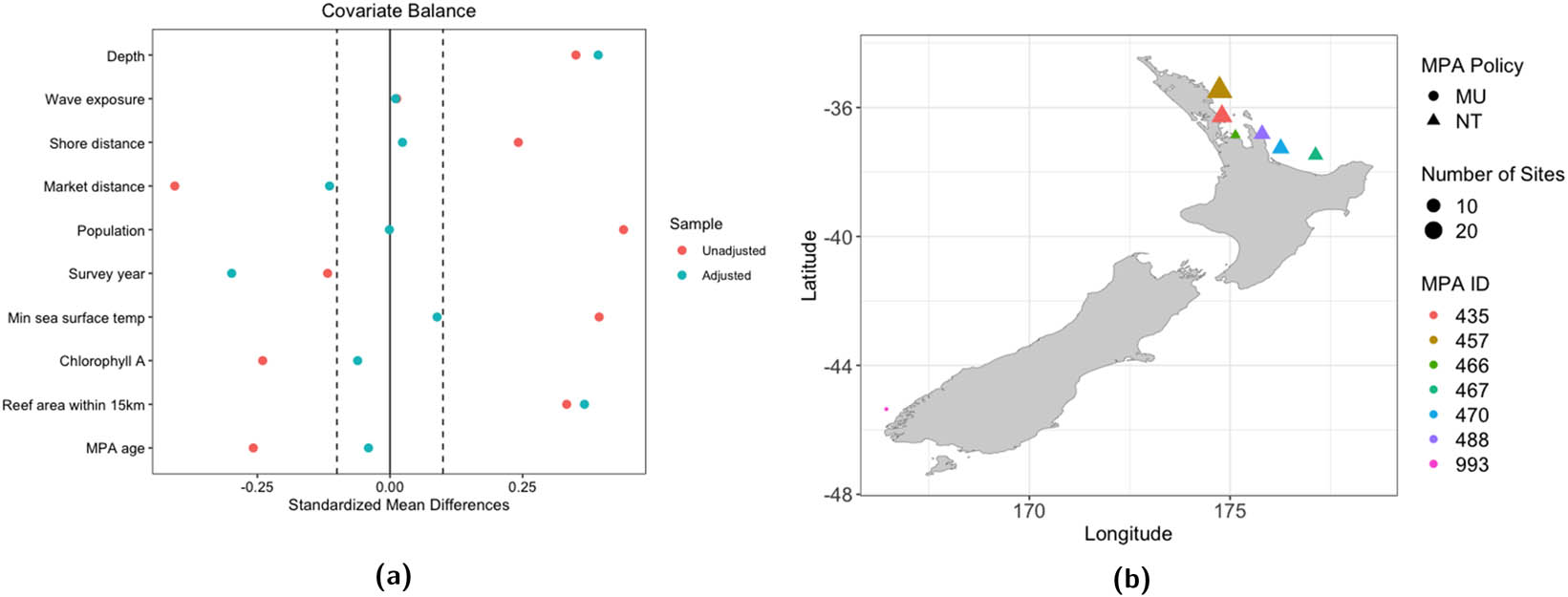
Challenges in MPA global dataset. (a) Covariate balance between unadjusted and adjusted situations and (b) MPAs in New Zealand.

3 Notation, assumptions, and estimands

To establish causal effect in clustered observational studies, we build our proposed matching strategy based on the potential outcomes framework [27–30], also known as the Neyman-Rubin causal model. Under the potential outcomes framework, the unit-level causal effect is defined as the difference between the outcomes under treatment and control in the same unit. Since we always observe only one of the outcomes for a single unit in reality, it is also considered a missing data problem.

Several works under the potential outcomes framework have been proposed for clustered data [11,13,31–35]. Distinguished from the existing literature, we focus on the setting where treatment is assigned at the cluster level and leverage the framework of matching estimators in the study by Abadie and Imbens [16] for causal inference.

Suppose for units i = 1 , … , N in cluster r = 1 , … , R , where the sample size of each cluster is n 1 , … , n r , respectively. Let Z r be a vector of cluster-level covariates and A r be the binary treatment indicator. To emphasize the role of cluster, we use X i , r ( i ) to denote the vector of unit-level covariates of the i th unit, where r = r ( i ) indicates the cluster it belongs to and thus is a function mapping from i ∈ { 1 , … , N } to r ∈ { 1 , … , R } . For simplicity, let X i r = X i , r ( i ) denote the unit-level covariates, and similarly, let Y i r ( a ) be the potential outcome receiving the treatment a ∈ { 0 , 1 } , and Y i r = Y i r ( A r ) be the observed outcome. Here, we suppose each unit belongs to only one cluster and clusters are not overlapped, i.e., N = n 1 + … + n R . Also, assume treatment is assigned at the cluster level, which implies that units within the same cluster are in the same treatment group. Supplementary Material Section 5 describes an extension to the case where the treatment varies within clusters.

To define the potential outcomes model, we introduce additional notation. Given X i r ∈ X , Z r ∈ Z and a ∈ { 0 , 1 } , we denote μ ( x , z , a ) = E [ Y i r ∣ X i r = x , Z r = z , A r = a ] , μ a ( x , z ) = E [ Y i r ( a ) ∣ X i r = x , Z r = z ] , σ 2 ( x , z , a ) = V [ Y i r ∣ X i r = x , Z r = z , A r = a ] , and σ a 2 ( x , z ) = V [ Y i r ( a ) ∣ X i r = x , Z r = z ] . Assume the following relationship between the potential outcome Y i r ( a ) and observed covariates X i r and Z r ,

where α r represents unobserved cluster-level random effect with mean 0, ε i r independently follows a distribution with mean 0 and variance σ 2 ( X i r , Z r , a ) for i = 1 , … , N and r = 1 , … , R . By including the cluster-level random effects, we impose a dependence structure for the error terms. Our goal is to estimate two aggregate estimands, i.e., the ATE and the average treatment effect for the treated (ATT). The ATE is defined as τ = E { Y ( 1 ) − Y ( 0 ) } , and the ATT is τ t = E { Y ( 1 ) − Y ( 0 ) ∣ A = 1 } .

We adopt the matching estimator proposed in Abadie and Imbens [16] and extend to clustered data. Each unit is matched to the closest M units in the opposite treatment group, where matching is done based on the Euclidean distance of the covariates. Denote J M ( i , r ) as the indices of the M matched units for unit i in the cluster r , and K M ( i , r ) be the number of times that unit i in cluster r is matched, i.e., K M ( i , r ) = ∑ l = 1 N ∑ k = 1 R I { ( i , r ) ∈ J M ( l , k ) } . Similar to X i r , r = r ( i ) in J M ( i , r ) and K M ( i , r ) denotes the cluster to which unit i belongs. In the double summation, we consider only the valid terms and disregard any undefined terms with incorrect cluster indices. Then the missing outcome for the unit i in cluster r can be imputed as follows:

To establish a valid causal effect in clustered data, we visit the necessary assumptions. We first retain the stable unit treatment values assumption (SUTVA), that is, the potential outcomes for each unit are not influenced by the treatment assigned to other units. While the SUTVA is a strong assumption, it is plausible in our case where most sites within one MPA received the same policy and MPAs are in general geographically separated from each other. We then modify the strong ignorability assumption in our setting, where treatments are assigned at the cluster level. Under the SUTVA and modified strong ignorability assumptions, μ ( x , z , a ) = μ a ( x , z ) and σ 2 ( x , z , a ) = σ a 2 ( x , z ) .

Assumption 1 suggests conditional independence between treatment A r and the potential outcome Y i r ( a ) when accounting for the cluster-level covariates Z r . It also requires overlap between treatment groups in the observed covariate distributions. The assumption of strong ignorability in (i) is untestable in practice. However, it is reasonable to proceed under this condition with enough knowledge on the treatment assignment mechanism and sufficient cluster-level covariates in the analysis. When treatment assignment occurs at the cluster level, individual-level covariates are not needed to achieve the strong ignorability assumption. For example, in the MPA dataset, sites within the same MPA typically receive the same policy, and the policy is determined by the MPA’s characteristics rather than site-specific covariates. Researchers can determine whether incorporating summary statistics of individual-level covariates is necessary

The matching estimator for the ATE in clustered data is

which can be rewritten as follows:

Note that the denominator is N instead of N R , because only one r = r ( i ) as the cluster index of unit i is included. Consequently, the total number of terms in the summation equals the total sample size N . Following a similar routine in unstructured data, we decompose the estimator τ ˆ mat as follows

where τ ( X , Z ) ¯ = N − 1 ∑ i = 1 N ∑ r = 1 R { μ 1 ( X i r , Z r ) − μ 0 ( X i r , Z r ) } represents the average conditional treatment effect, E M = N − 1 ∑ i = 1 N ∑ r = 1 R ( 2 A r − 1 ) { 1 + K M ( i , r ) ⁄ M } { Y i r − μ A r ( X i r , Z r ) } is a weighted average of the residuals, and the conditional bias relative to τ ( X , Z ) ¯ is B M = N − 1 ∑ i = 1 N ∑ r = 1 R ( 2 A r − 1 ) M − 1 ∑ ( j , k ) ∈ J M ( i , r ) { μ 1 − A r ( X i r , Z r ) − μ 1 − A r ( X j k , Z k ) } .

For the ATT in clustered data, the strong ignorability assumption can be relaxed as in the unstructured data as well.

The estimator of the ATT can be written as follows:

where N 1 is the number of subjects receiving treatment 1. Similar to the decomposition for the ATE estimator,

where τ ( X ) ¯ t = N 1 − 1 ∑ i = 1 N ∑ r = 1 R A r { μ ( X i r , Z r , 1 ) − μ 0 ( X i r , Z r ) } , E M t = N 1 − 1 ∑ i = 1 N ∑ r = 1 R { A r − ( 1 − A r ) K M ( i , r ) ⁄ M } { Y i r − μ A r ( X i r , Z r ) } , and B M t = N 1 − 1 ∑ i = 1 N ∑ r = 1 R A r M − 1 ∑ ( j , k ) ∈ J M ( i , r ) { μ 0 ( X i r , Z r ) − μ 0 ( X j k , Z k ) } .

Consistent with the findings in unstructured data, the matching discrepancies of the ATE and ATT estimators come from the conditional bias terms B M and B M t , which need careful consideration when matching on multiple covariates. According to Abadie and Imbens [16], B M = O p ( N − 1 ⁄ k ) such that the asymptotic distribution of the ATE estimator can be dominated by the bias when matching on k > 1 covariates. Similar rates apply for the ATT estimator, where B M t = O p ( N 1 − r ⁄ k ) for some r ≥ 1 . Since we consider matching on both cluster-level and unit-level covariates, such bias terms are non-negligible. For instance, in Figure 2(a), although matching reduces covariate imbalance to a large extent, certain covariate imbalance still persists. Following Abadie and Imbens [17], we work on the bias-corrected estimators instead. Denote τ ˆ and τ ˆ t as the bias-corrected estimators for ATE and ATT, we have

and τ ˆ t = τ ˆ mat t − B ˆ M t = τ ˆ mat t − N − 1 ∑ i = 1 N ∑ r = 1 R A r M − 1 ∑ ( j , k ) ∈ J M ( i , r ) { μ ˆ 0 ( X i r , Z r ) − μ ˆ 0 ( X j k , Z k ) } , where μ ˆ A r ( X i r , Z r ) is a consistent estimator of μ A r ( X i r , Z r ) .

4 Large sample properties

In our clustered data setting, matching on cluster-level covariates is sufficient to account for the confounding variables. However, motivated by blocked randomized experimental designs, matching on both cluster-level and unit-level covariates may improve efficiency. To compare the two matching schemes, we denote S as a unified variable representing either the cluster-level covariates or both cluster-level and unit-level covariates to be matched on. We explore the asymptotic normality under the fixed M matches for the bias-corrected matching estimators. We then illustrate the benefits of matching on both cluster-level and unit-level covariates based on the asymptotic variance. Following Abadie and Imbens [16], we extend necessary assumptions for independent and identically distributed data to clustered data (details can be found in Supplementary Material S1).

To illustrate the role of the matching scheme, for a general random variable S , we further define μ a ( S ) = E [ Y i r ( a ) ∣ S ] and τ ( S ) = μ 1 ( S ) − μ 0 ( S ) as the conditional mean outcome and treatment effect functions. Denote the variance terms V τ ( S ) = E [ ( τ ( S ) − τ ) 2 ] , V τ ( S ) , t = E [ ( τ ( S ) t − τ t ) 2 ] , V E = plim N − 1 ∑ i = 1 N ∑ r = 1 R { 1 + M − 1 K M ( i , r ) } 2 V [ Y i r − μ A r ( S i r ) ] , and V E , t = plim N 1 − 1 ∑ i = 1 N ∑ r = 1 R { A r − ( 1 − A r ) M − 1 K M ( i , r ) } 2 V [ Y i r − μ A r ( S i r ) ] , we establish the asymptotic normality for bias-corrected estimators in Theorems 1 and 2 (see proofs in Supplementary Material S2).

The asymptotic variances for the two estimators involve the variances of residual terms, i.e., V E and V E , t . Specifically, we have

Consider two matching schemes, i.e., S = ( X , Z ) and S = Z , we note that for V [ Y i r − μ A r ( X i r , Z r ) ] and V [ Y i r − μ A r ( Z r ) ] , when unit-level covariates provide valuable information to the outcome Y i r , matching on both cluster-level and unit-level covariates results in lower residual variance than matching on cluster-level covariates. Despite the increased number of covariates for matching, the bias correction helps remove the conditional bias. Hence, we recommend that matching on both cluster-level and unit-level covariates is more efficient when the unit-level information is available.

5 Variance estimation

Variance estimation for matching estimators has been investigated in both parametric and nonparametric ways. In the study by Abadie and Imbens [16], an analytic form for the large sample variance is proposed with consistency achieved. Although the bootstrap method [36] is widely used to calculate standard errors for estimators with complicated forms, Abadie and Imbens [20] showed that the standard bootstrap is invalid for matching estimators. The bootstrap method does not preserve the distribution of K M ( i ) , which follows a Binomial distribution. To overcome this challenge, statistical tools, including wild bootstrap [37] and weighted bootstrap methods [19], are developed to estimate asymptotic variance for matching estimators. The weighted bootstrap method [19] can be used when matching is directly performed on covariates, while the wild bootstrap [37] is applied based on the estimated propensity score. Both methods apply to unstructured data. As for clustered data, there are two main bootstrap strategies: (i) two-stage bootstrap, which is to resample entire clusters at first and then resample subjects within the selected clusters, and (ii) cluster bootstrap, which resamples entire clusters and includes all subjects from the selected clusters. Davison and Hinkley [18] discussed different bootstrap methods and showed that the latter is preferable theoretically in clustered data. Recent studies suggested that allowing the number of matches to grow with the sample size can address the invalidity of the bootstrap [38]. However, it remains challenging to determine how many matches are sufficient to ensure the bootstrap’s validity in a given finite sample dataset.

Due to the complex analytic form of matching estimators in clustered data, we employ resampling methods to estimate the variance of the matching estimator and leverage the general procedure of the weighted bootstrap. To account for the dependence in the linear terms in the weighted bootstrap, we incorporate the cluster bootstrap for variance estimation. We describe the extension of weighted bootstrap in clustered data for the ATE first and present the procedure for our cluster weighted bootstrap method. A similar procedure for the ATT is summarized in Supplementary Material S4.

Theorem 1 states that under certain conditions, the bias-corrected estimator τ ˆ is asymptotically normal: N ( τ ˆ − τ ) ⁄ σ → d N ( 0 , 1 ) , where σ 2 = σ 1 2 + σ 2 2 . The asymptotic variance σ 2 consists of two parts, i.e.,

where σ 1 2 measures the variability of τ ( S ) ¯ − τ and σ 2 2 captures the variability of weighted average of the residuals E M . By following Otsu and Rai [19], we write our bias-corrected estimator τ ˆ = τ ˆ mat − B ˆ M as a linear form in clustered data,

where τ ˆ i = ∑ r = 1 R { μ ˆ 1 ( S i r ) − μ ˆ 0 ( S i r ) } + ( 2 A r − 1 ) { 1 + M − 1 K M ( i , r ) } { Y i r − μ ˆ A r ( S i r ) } .

On the basis of this form, we express the i th residual as τ ˆ i − τ ˆ = ξ ˆ i + e ˆ i with ξ ˆ i and e ˆ i are estimated values of ξ i = ∑ r = 1 R { μ A r ( S i r ) − μ 1 − A r ( S i r ) } − τ and e i = ∑ r = 1 R ( 2 A r − 1 ) { 1 + M − 1 K M ( i , r ) } { Y i r − μ A r ( S i r ) } , respectively. This form is the key aspect to obtain the estimated variance for matching estimators. A cluster-robust variance estimator V ˆ CRV E can be computed as follows:

where

and τ ˆ ¯ r ′ = n r ′ − 1 ∑ i : r ( i ) = r ′ τ ˆ i is the cluster mean. This estimator accounts for within-cluster dependence and provides a consistent variance estimate for the matching estimator.

Alternatively, we propose a cluster-level weighted bootstrap method following Otsu and Rai [19]. The key idea is to treat { τ ˆ i } i = 1 N as observations, ensuring that the distribution of K M ( i ) is preserved. Bootstrapping on { τ ˆ i } i = 1 N therefore provides a valid variance estimate. While the weighted bootstrap estimator ultimately aligns with the cluster-robust variance estimator based on the standard sample variance structure [39], we recommend using bootstrap methods to enhance finite-sample performance. Prior research has demonstrated the strong finite-sample properties of wild bootstrap methods in classical settings such as linear regression [40]. Other studies have also shown that bootstrap-based approaches perform well in situations with a small number of clusters or unbalanced cluster sizes [41–43]. On the basis of the literature, we believe that the proposed cluster bootstrap procedure is likely to exhibit good finite-sample performance in practice. Moreover, the bootstrap estimator is both convenient and easy to implement.

Considering the clustered data where unobserved cluster-level confounding covariates could exist across and within clusters, we adopt the cluster bootstrap method [18] to account for the variance from potential cluster-level covariates. The cluster bootstrap suggests resampling on the cluster levels first and then including all observations within selected units. By incorporating the weighted bootstrap algorithm, we propose our cluster-weighted bootstrap method as follows. The weights can be generated from multinomial random variables { M i * } i = 1 N .

1. Step 1: Obtain the weighted bootstrap samples { τ ˆ i } i = 1 N based on the matching estimator framework.

2. Step 2: For clustered data with n observations and R non-overlapped clusters, sample R clusters with replacement.

3. Step 3: Include all { τ ˆ i } i = 1 N within selected clusters and calculate their corresponding weights { W i * } i = 1 N . One option of generating weights is to set W i * = M i * ⁄ N , where ( M 1 * , … , M N * ) is a vector from a multinomial distribution with equal probability.

4. Step 4: Obtain a bootstrap replicate as τ ˆ b * = ∑ i = 1 N W i * ( τ ˆ i − τ ˆ ) .

5. Step 5: Repeat the Step 1–4 B times. Compute the bootstrap variance estimator for the bias-corrected matching estimator τ ˆ as the empirical variance of { τ ˆ b * } b = 1 B .

Proof for Theorem 3 is detailed in Supplementary Material S3.

6 Analysis of conservation policy effects on marine biodiversity

The proposed matching framework is applied to the Gill et al.’s [6] MPA dataset to investigate the causal relationship between MPA policies and fish biodiversity. We consider MU as the treatment while the NT serves as the control. Two estimands are of interest, i.e., ATE = E [ Y ( MU ) − Y ( NT ) ] and ATT = E [ Y ( MU ) − Y ( NT ) ∣ A = MU ] . We impute the missing counterfactual for each site by matching with replacement and with a fixed number of matches. The Mahalanobis distance metric is calculated to measure the similarity of sites under different policies. Three nearest control sites are matched to the treatment site. Due to the skewed covariates distributions between two groups, we transform the non-negative continuous covariates by the Box-Cox transformation. The outcome of interest is the log transformation of fish biomass ( g ⁄ 100 m 2 ). Following our recommendation, matching is conducted on both MPA-level and site-level covariates, and the performance is compared to matching on MPA-level covariates. The mean outcome functions are estimated by three methods: (i) the spline regression [44], (ii) the sieve method [45], and (iii) the regression forest [46]. Because of the large number of first-order and second-order terms among covariates, we apply the LASSO method [47] to select a subset of covariates before matching [48,49]. The regularization parameter is chosen by fivefold cross validation and the bias-corrected estimators for the ATE and ATT are derived. Corresponding variances are computed by the proposed cluster-weighted bootstrap method.

Table 2 summarizes the estimated ATE and ATT with 95% confidence intervals under different matching strategies. When matching only on MPA-level covariates, all three methods result in negative point estimates for ATE and ATT. However, none detect significant differences between the MU and NT policy on fish biomass. When matching on both MPA-level and site-level covariates, the sieve method shows significantly different impacts of MPA policies on fish biomass. The ATE under the sieve method is significantly negative, suggesting that the NT policy is more beneficial to fish biodiversity. The result of the ATT by using the sieve method is consistent with the ATE result, which shows a positive impact of using the NT policy. Comparing the procedures between matching on MPA-level covariates and matching on all relevant covariates, we find a reduced estimated variance under the sieve method as expected when including individual covariates that are relevant to the outcome.

In these MPA data, several site-level covariates such as distance to markets, reef area within 15 km, and neighboring human population size are relevant to the fish biodiversity under either the MU or NT policy (Figure S2 in Supplementary Material S6). Certain regions at the habitat, country and ecoregion levels also show an important association with the fish biodiversity. Taking these covariates into account for matching helps reduce the matching variance. Using the regression forest method also reveals the beneficial effect of the NT policy for the estimated ATE, while the effect is barely detected for the ATT.

7 Simulation study

We conduct a simulation study to evaluate the finite-sample performance of matching estimators when matching on cluster-level covariates only or matching on both cluster-level and unit-level covariates, and compare the proposed cluster weighted bootstrap method with the original weighted bootstrap on variance estimation. Table 3 outlines the two data-generating processes – balanced and unbalanced designs – and the 12 matching estimators, which vary based on the choice of nuisance function estimation, covariates used for matching, and method for variance estimation. Table 4 summarizes the results under different scenarios for the ATE. When matching on the cluster-level covariate, the small biases for both balanced and unbalanced cluster size settings suggest that matching on the cluster-level covariate is sufficient to remove estimation bias for the treatment effect. It is also consistent with the theoretical findings by Abadie and Imbens [16] that the conditional bias is ignorable when matching on a single covariate. When comparing three approaches to approximate the conditional outcome mean functions, the sieve method usually outperforms the other two with the lowest bias. The linear spline method shows advantages in reducing the bias for unbalanced data but suffers from underestimated variance. The regression forest method has the largest absolute bias in most cases.

As for variance estimation, the standard weighted bootstrap always results in a much smaller variance than the cluster-weighted bootstrap and thus lower coverage for the 95% confidence interval. By ignoring the cluster effect, the weighted bootstrap method resamples on the unit level such that it fails to approximate the true distribution of matching estimators. On the contrary, by taking clusters into consideration and resampling at the cluster level, our proposed cluster-weighted bootstrap method results in high coverage for the 95% confidence interval.

Comparing procedures 1 and 3, the estimated variances when using both cluster and unit covariates for matching are always smaller than those using only the cluster-level covariate for matching. Though matching on the cluster-level covariate leads to small biases, the consistently reduced estimated variances suggest matching on both cluster-level and unit-level covariates is beneficial and can achieve high coverage for the 95% confidence interval.

When estimating the ATT (Table 5), the sieve method still achieves the most accurate estimation and usually the highest coverage probability. When matching on both cluster and unit covariates, the estimated variance is lower than matching on the cluster-level covariate, and the coverages for the 95% confidence interval are as close to 95% as those when matching on the cluster-level covariate.

References

[1] Grorud-Colvert K, Sullivan-Stack J, Roberts C, Constant V, e Costa BH, Pike EP, et al. The MPA guide: A framework to achieve global goals for the ocean. Science. 2021;373(6560):eabf0861. 10.1126/science.abf0861Search in Google Scholar PubMed
[2] UNEP-WCMC, IUCN, NGS. Protected Planet Live Report 2021. Cambridge UK; Gland, Switzerland; and Washington, D.C., USA; 2021. Search in Google Scholar
[3] Ferraro PJ, Sanchirico JN, Smith MD. Causal inference in coupled human and natural systems. Proc Nat Acad Sci USA. 2019;116(12):5311–8. 10.1073/pnas.1805563115Search in Google Scholar PubMed PubMed Central
[4] Kamat V. The ocean is our farm: Marine conservation, food insecurity, and social suffering in Southeastern Tanzania. Human Organization. 2014;73(3):289–98. 10.17730/humo.73.3.f43k115544761g0vSearch in Google Scholar
[5] Bennett NJ, Dearden P. Why local people do not support conservation: Community perceptions of marine protected area livelihood impacts, governance and management in Thailand. Marine Policy. 2014;44:107–16. 10.1016/j.marpol.2013.08.017Search in Google Scholar
[6] Gill DA, Mascia MB, Ahmadia GN, Glew L, Lester SE, Barnes M, et al. Capacity shortfalls hinder the performance of marine protected areas globally. Nature. 2017;543(7647):665–9. 10.1038/nature21708Search in Google Scholar PubMed
[7] Pynegar EL, Gibbons JM, Asquith NM, Jones JPG. What role should randomized control trials play in providing the evidence base for conservation? Oryx. 2021;55(2):235–44. 10.1017/S0030605319000188Search in Google Scholar
[8] Stuart EA. Matching methods for causal inference: A review and a look forward. Stat Sci Rev J Instit Math Stat. 2010;25(1):1–21. 10.1214/09-STS313Search in Google Scholar PubMed PubMed Central
[9] Cafri G, Wang W, Chan PH, Austin PC. A review and empirical comparison of causal inference methods for clustered observational data with application to the evaluation of the effectiveness of medical devices. Stat Meth Med Res. 2019;28(10-11):3142–62. 10.1177/0962280218799540Search in Google Scholar PubMed
[10] Zubizarreta JR, Keele L. Optimal multilevel matching in clustered observational studies: a case study of the effectiveness of private schools under a large-scale voucher system. J Am Stat Assoc. 2017;212(518):547–60. 10.1080/01621459.2016.1240683Search in Google Scholar
[11] Hong G, Raudenbush SW. Evaluating Kindergarten retention policy: a case study of causal inference for multilevel observational data. J Am Stat Assoc. 2006;101(475):901–10. 10.1198/016214506000000447Search in Google Scholar
[12] Arpino B, Mealli F. The specification of the propensity score in multilevel observational studies. Comput Stat Data Anal. 2011;55(4):1770–80. 10.1016/j.csda.2010.11.008Search in Google Scholar
[13] Yang S. Propensity score weighting for causal inference with clustered data. J Causal Inference. 2018;6(2):20170027. 10.1515/jci-2017-0027Search in Google Scholar
[14] Chang TH, Stuart EA. Propensity score methods for observational studies with clustered data: A review. Stat Med. 2022;41(18):3612–26. 10.1002/sim.9437Search in Google Scholar PubMed PubMed Central
[15] King G, Nielsen R. Why propensity scores should not be used for matching. Politic Anal. 2019;27(4):435–54. 10.1017/pan.2019.11Search in Google Scholar
[16] Abadie A, Imbens GW. Large sample properties of matching estimators for average treatment effects. Econometrica. 2006;74(1):235–67. 10.1111/j.1468-0262.2006.00655.xSearch in Google Scholar
[17] Abadie A, Imbens GW. Bias-corrected matching estimators for average treatment effects. J Business Econ Stat. 2011;29(1):1–11. 10.1198/jbes.2009.07333Search in Google Scholar
[18] Davison AC, Hinkley DV. Bootstrap Methods and their Application. Cambridge Series in Statistical and Probabilistic Mathematics. Cambridge: Cambridge University Press; 1997. Search in Google Scholar
[19] Otsu T, Rai Y. Bootstrap inference of matching estimators for average treatment effects. J Am Stat Assoc. 2017;112(520):1720–32. 10.1080/01621459.2016.1231613Search in Google Scholar
[20] Abadie A, Imbens GW. On the failure of the bootstrap for matching estimators. Econometrica. 2008;76(6):1537–57. 10.3982/ECTA6474Search in Google Scholar
[21] Ahmadia G, Glew L, Provost M, Gill D, Hidayat N, Mangubhai S, et al. Integrating impact evaluation in the design and implementation of monitoring marine protected areas. Phil Trans R Soc B. 2015;370:20140275. 10.1098/rstb.2014.0275Search in Google Scholar PubMed PubMed Central
[22] Brewer TD, Cinner JE, Green A, Pressey RL. Effects of human population density and proximity to markets on coral reef fishes vulnerable to extinction by fishing. Conservat Biol. 2013;27(3):443–52. 10.1111/j.1523-1739.2012.01963.xSearch in Google Scholar PubMed
[23] Edgar GJ, Stuart-Smith RD, Willis TJ, Kininmonth S, Baker S, Barrett N, et al. Global conservation outcomes depend on marine protected areas with five key features. Nature 2014;506:216–220. 10.1038/nature13022Search in Google Scholar PubMed
[24] Campbell SJ, Darling ES, Pardede S, Ahmadia G, Mangubhai S, Amkieltiela, et al. Fishing restrictions and remoteness deliver conservation outcomes for Indonesia’s coral reef fisheries. Conservation Letters. 2020;13(2):e12698. 10.1111/conl.12698Search in Google Scholar
[25] Toth LT, van Woesik R, Murdoch TJT, Smith SR, Ogden J, Precht WF, et al. Do no-take reserves benefit Florida’s corals? 14 years of change and stasis in the Florida Keys National Marine Sanctuary. Coral Reefs. 2014;33:565–77. 10.1007/s00338-014-1158-xSearch in Google Scholar
[26] Karr KA, Fujita R, Halpern BS, Kappel CV, Crowder L, Selkoe KA, et al. Thresholds in Caribbean coral reefs: implications for ecosystem-based fishery management. J Appl Ecol. 2015;52(2):402–12. 10.1111/1365-2664.12388Search in Google Scholar
[27] Rubin DB. Estimating Causal Effects of Treatments in Randomized and Nonrandomized Studies. J Educ Psychol. 1974;66(5):688–701. 10.1037/h0037350Search in Google Scholar
[28] Holland PW. Statistics and causal inference. J Am Stat Assoc. 1986;81(396):945–60. 10.1080/01621459.1986.10478354Search in Google Scholar
[29] Splawa-Neyman J, Dabrowska DM, Speed TP. On the application of probability theory to agricultural experiments. Essay on principles. Section 9. Stat Sci. 1990;5(4):465–72. 10.1214/ss/1177012031Search in Google Scholar
[30] Rosenbaum PR, Rubin DB. The central role of the propensity score in observational studies for causal effects. Biometrika. 1983;70(1):41–55. 10.1093/biomet/70.1.41Search in Google Scholar
[31] Stuart EA. Estimating causal effects using school-level data sets. Educ Res. 2007;36(4):187–98. 10.3102/0013189X07303396Search in Google Scholar
[32] VanderWeele TJ. Ignorability and stability assumptions in neighborhood effects research. Stat Med. 2008;27(11):1934–43. 10.1002/sim.3139Search in Google Scholar PubMed
[33] Li F, Zaslavsky AM, Landrum MB. Propensity score weighting with multilevel data. Stat Med. 2013;101(19):3373–87 10.48550/arXiv.1808.01647.Search in Google Scholar
[34] He Z. Inverse conditional probability weighting with clustered data in causal inference; 2018. Search in Google Scholar
[35] Lee Y, Nguyen TQ, Stuart EA. Partially pooled propensity score models for average treatment effect estimation with multilevel data. J R Stat Soc Ser A (Stat Soc). 2021;184(4):1578–98. 10.1111/rssa.12741Search in Google Scholar
[36] Efron B. Bootstrap methods: another look at the Jackknife. Ann Stat. 1979;7(1):1–26. 10.1214/aos/1176344552Search in Google Scholar
[37] Huber M, Camponovo L, Bodory H, Lechner M. A wild bootstrap algorithm for propensity score matching estimators. Faculty of Economics and Social Sciences, University of Freiburg/Fribourg Switzerland; 2016. p. 470. Search in Google Scholar
[38] Lin Z, Ding P, Han F. Estimation based on nearest neighbor matching: from density ratio to average treatment effect. Econometrica. 2023;91(6):2187–217. 10.3982/ECTA20598Search in Google Scholar
[39] Ding P. A first course in causal inference. New York, NY, USA: CRC Press; 2024. 10.1201/9781003484080Search in Google Scholar
[40] Mammen E. Bootstrap and wild bootstrap for high dimensional linear models. An Stat. 1993;21(1):255–85. 10.1214/aos/1176349025Search in Google Scholar
[41] Cameron AC, Gelbach JB, Miller DL. Bootstrap-based improvements for inference with clustered errors. Rev Econ Stat. 2008;90(3):414–27. 10.1162/rest.90.3.414Search in Google Scholar
[42] Cameron AC, Miller DL. A practitioner’s guide to cluster-robust inference. J Human Resources. 2015;50(2):317–72. 10.3368/jhr.50.2.317Search in Google Scholar
[43] MacKinnon JG, Nielsen MØ, Webb MD. Fast and reliable jackknife and bootstrap methods for cluster-robust inference. J Appl Econ. 2023;38(5):671–94. 10.1002/jae.2969Search in Google Scholar
[44] Schoenberg IJ. Contributions to the problem of approximation of equidistant data by analytic functions: Part A. on the problem of smoothing or graduation. a first class of analytic approximation formulae. Quarter Appl Math. 1946;4(1):45–99. 10.1090/qam/15914Search in Google Scholar
[45] Chen X. Chapter 76 Large sample sieve estimation of semi-nonparametric models. In: Handbook of econometrics. vol. 6. Elsevier; 2007. p. 5549–632. 10.1016/S1573-4412(07)06076-XSearch in Google Scholar
[46] Athey S, Tibshirani J, Wager S. Generalized random forests. Ann Stat. 2019;47(2):1148–78. 10.1214/18-AOS1709Search in Google Scholar
[47] Tibshirani R. Regression shrinkage and selection via the Lasso. J R Stat Soc Ser B (Methodological). 1996;58(1):267–88. 10.1111/j.2517-6161.1996.tb02080.xSearch in Google Scholar
[48] Zhang Y, Yang S, Ye W, Faries DE, Lipkovich I, Kadziola Z. Practical recommendations on double score matching for estimating causal effects. Stat Med. 2022;41(8):1421–45. 10.1002/sim.9289Search in Google Scholar PubMed PubMed Central
[49] Zhao H, Yang S. Outcome-adjusted balance measure for generalized propensity score model selection. J Stat Plan Inference. 2022;221:188–200. 10.1016/j.jspi.2022.04.004Search in Google Scholar
[50] Yang S, Zhang Y. Multiply robust matching estimators of average and quantile treatment effects. Scand J Stat. 2023;50(1):235–65. 10.1111/sjos.12585Search in Google Scholar PubMed PubMed Central
[51] Yang S, Lok JJ. Sensitivity analysis for unmeasured confounding in coarse structural nested mean models. Stat Sin. 2018;28(4):1703–23. 10.5705/ss.202016.0133Search in Google Scholar PubMed PubMed Central
© 2025 the author(s), published by De Gruyter
This work is licensed under the Creative Commons Attribution 4.0 International License.
Articles in the same Issue
- Research Articles
- Decision making, symmetry and structure: Justifying causal interventions
- Targeted maximum likelihood based estimation for longitudinal mediation analysis
- Optimal precision of coarse structural nested mean models to estimate the effect of initiating ART in early and acute HIV infection
- Targeting mediating mechanisms of social disparities with an interventional effects framework, applied to the gender pay gap in Western Germany
- Role of placebo samples in observational studies
- Combining observational and experimental data for causal inference considering data privacy
- Recovery and inference of causal effects with sequential adjustment for confounding and attrition
- Conservative inference for counterfactuals
- Treatment effect estimation with observational network data using machine learning
- Causal structure learning in directed, possibly cyclic, graphical models
- Mediated probabilities of causation
- Beyond conditional averages: Estimating the individual causal effect distribution