Variable importance for causal forests: breaking down the heterogeneity of treatment effects
-
Clément Bénard


Abstract
Causal random forests provide efficient estimates of heterogeneous treatment effects. However, forest algorithms are also well-known for their black-box nature, and therefore, do not characterize how input variables are involved in treatment effect heterogeneity, which is a strong practical limitation. In this article, we develop a new importance variable algorithm for causal forests, to quantify the impact of each input on the heterogeneity of treatment effects. The proposed approach is inspired from the drop and relearn principle, widely used for regression problems. Importantly, we show how to handle the case where the forest is retrained without a confounding variable. If the confounder is not involved in the treatment effect heterogeneity, the local centering step enforces consistency of the importance measure. Otherwise, when a confounder also impacts heterogeneity, we introduce a corrective term in the retrained causal forest to recover consistency. Additionally, experiments on simulated, semi-synthetic, and real data show the good performance of our importance measure, which outperforms competitors on several test cases. Experiments also show that our approach can be efficiently extended to groups of variables, providing key insights in practice.
1 Introduction
1.1 Context and objectives
Estimating heterogeneous treatment effects has recently attracted a great deal of interest in the machine learning community, particularly for medical applications [1] and in the social sciences. Over the past few years, numerous efficient algorithms have been developed to estimate such effects, including double robust methods [2], R-learners [3], X-learners [4], causal forests [5], 6], the lasso [7], BART [8], or neural networks [9]. Besides, let us also mention policy learning, which aims at selecting relevant individuals to treat [10], [11], [12], [13]. However, most of these methods remain black boxes, and it is therefore difficult to grasp how input variables impact treatment effects. This understanding is crucial for optimizing treatment policies, for instance, so that this shortcoming clearly limits their practical use. While the accuracy of treatment effect estimates has significantly improved recently, little effort has been dedicated to improve their interpretability, and quantifying the impact of variables involved in treatment effect heterogeneity. In this regard, we can mention the importance measure of the causal forest package grf [14], the double robust approach of [15], and the algorithm from [16] for high dimensional linear cases. The main purpose of this article is to introduce a variable importance measure for heterogeneous treatment effects, improving over the existing algorithms, to better identify the sources of heterogeneity. We focus on causal random forests, defined as a specific case of generalized forests [6], and well-known to be one of most powerful algorithm to estimate heterogeneous treatment effects.
1.1.1 Contributions
Our main contribution is thus the introduction of a variable importance algorithm for causal random forests, following the drop and retrain principle, which is well-established for regression problems [17], [18], [19], [20]. The main idea is to retrain the learning algorithm without a given input variable, and measure the drop of accuracy to get its importance. In particular, such approach ensures that irrelevant variables get a null importance asymptotically. In the context of causal inference, the main obstacle is to retrain the causal forest without a confounding variable, since the unconfoundedness assumption can be violated, leading to inconsistent forest estimates and biased importance values, as explained in Section 2. However, we will see that the local centering of the outcome and treatment assignment leads to consistent estimates, provided that the removed variable is not involved in the treatment effect heterogeneity. Otherwise, to handle a confounder involved in heterogeneity, we introduce a corrective term in the retrained causal forest. Overall, we will show in Section 3, that our proposed variable importance algorithm is consistent, under standard assumptions in the literature about the theoretical analysis of random forests. Next, in Section 4, we run several batches of experiments on simulated, semi-synthetic, and real data to show the good performance of the introduced method compared to the existing competitors. Additionally, we take advantage of the experimental section to illustrate that the extension of our approach to group of variables is straightforward and provides powerful insights in practice. The remaining of this first section is dedicated to the mathematical formalization of the problem.
1.2 Definitions
To define heterogeneous treatment effects, we first introduce a standard causal setting with an input vector
where μ(X) is a baseline function,
The cornerstone of causal treatment effect identifiability is the assumption of unconfoundedness given in Assumption 1, which states that all confounding variables are observed in the data. By definition, the responses Y(0), Y(1), and the treatment assignment W simultaneously depend on the confounding variables. If all confounding variables are observed, then the responses and the treatment assignment are independent conditional on the inputs. Consequently, the treatment effect is identifiable, as stated in Proposition 1 below—all proofs of propositions and theorems stated throughout the article are gathered in Appendix A. Notice that Assumption 1 below enforces that the input vector X contains all confounding variables, but X may also contain non-confounding variables. Consequently,
Assumption 1.
Potential outcomes are independent of the treatment assignment conditional on the observed input variables, i.e., Y(0), Y(1) ⊥⊥ W∣X.
Proposition 1.
If the unconfoundedness Assumption 1 is satisfied, then we have
Note that we define above the treatment effect as the expected difference between potential outcomes, conditioned on input variables. However, the heterogeneity properties strongly depend on how we define the treatment effect [21], [22], [23]. The ratio between the means of potential outcomes may also define a treatment effect, leading to potential heterogeneity while our original outcome difference remains constant. A thorough discussion of this topic is out of scope of this article, and we take the difference of potential outcomes as treatment effect, the widely used metric for many applications [21]. We refer to Colnet et al. [23] for a comparison of treatment effect measures.
VanderWeele and Robins [21] defined treatment effect heterogeneity as follows.
Definition 1:
(VanderWeele and Robins [21]). The treatment effect τ is said to be heterogeneous with respect to X if it exists
We strengthen this definition in two directions, formalized in Definition 2 below. First, we require τ to be heterogeneous with respect to each variable in
Definition 2.
The treatment effect τ is said to be heterogeneous with respect to all variables in
with x′(−j) = x
(−j), and
In the sequel, we assume that the treatment effect τ is heterogeneous in the sense of Definition 2, and that X admits a strictly positive density, to enforce heterogeneity with a positive probability, as stated in the proposition below. Our objective is to quantify the influence of the input variables X on the treatment heterogeneity using an available sample
Assumption 2.
The treatment effect τ is heterogeneous according to Definition 2, and X admits a strictly positive density.
Proposition 2.
If Assumption 2 is satisfied, and X′ is an independent copy of X, then
2 Variable importance for heterogeneous treatment effects
2.1 Theoretical definition
To propose a variable importance measure, we build on Sobol [24] and Williamson et al. [18], which define variable importance in the case of regression as the proportion of output explained variance lost when a given input variable is removed. Hines et al. [15] extend this idea to treatment effects, and introduce the theoretical importance measure I(j) of X (j), defined by
which is well-defined under Assumption 2, since
Proposition 3.
Let Assumption 2 be satisfied. If
Note that by definition of I(j), a variable strongly correlated to another variable involved in the heterogeneity, has a low importance value. This is due to the fact that, owing to this strong dependence, there is minimal loss of information regarding the treatment effect heterogeneity when such a variable is removed. As suggested by both Williamson et al. [18] and Hines et al. [15], one possible approach involves extending the importance measure to a group of variables, where strongly dependent variables are grouped together. For the sake of clarity, we focus on the case of a single variable in the following sections. However, extending this approach to groups of variables is straightforward, and we will present such examples in the experimental section.
More importantly, Hines et al. [15] highlight that a key problem to estimate the above quantity I(j), is that the unconfoundedness Assumption 1 does not imply unconfoundedness for the reduce set of input variables X
(−j), i.e., we may have Y(0), Y(1)⊥̸⊥W∣X
(−j). Hines et al. [15] overcome this issue using double robust approaches [2], 3] to estimate τ with all input variables in a first step, and then regress the obtained treatment effect on X
(−j) to estimate
2.2 Causal random forests
Generalized random forests [6] are a generic framework to build efficient estimates of quantities defined as solutions of local moment equations. As opposed to original Breiman’s forests, generalized forests are not the average of tree outputs. Instead, trees are aggregated to generate weights for each observation of the training data, used in a second step to build a weighted estimate of the target quantity. Causal forests are a specific case of generalized forest, where the following local moment equation identifies the treatment effect under the unconfoundedness Assumption (1),
The local moment Equation (3) is thus used to define the causal forest estimate τ
M,n
(x) at a new query point x, built from the data
where
Finally, the causal forest algorithm first performs a local centering step in practice, by regressing Y and W on X using regression forests, fit with
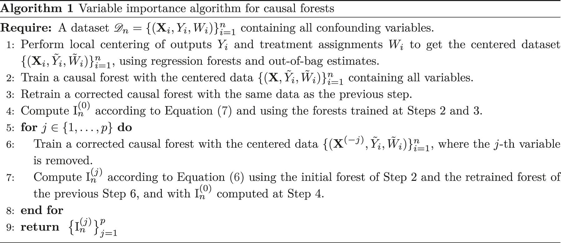
2.3 Variable importance algorithm
We take advantage of causal forests to build an estimate of our variable importance measure I(j), defined in Equation (2). The forest estimate τ
M,n
(x), described in the previous subsection, provides a plug-in estimate for the first term
2.3.1 Identifiability of treatment effect
When a variable X
(j) is removed from the input variables, the moment Equation (3) does not necessarely hold anymore, since unconfoundedness Assumption (1) may be violated with a reduced set of inputs, even for
Proposition 4.
If Assumption 1 is satisfied, we have
which is the local moment equation defining causal forests, with input variables
On the other hand, removing an influential and confounding variable
Proposition 5.
If Assumption 1 is satisfied, then we have for
Then, for a query point x
(−j) ∈ [0,1]
p−1, if
Athey and Wager [25], Footnote 5, page 42] conduct an empirical analysis using causal forests, and state in a footnote, that local centering “eliminates confounding effects. Thus, we do not need to give the causal forest all features X
(j) that may be confounders. Rather, we can focus on features that we believe may be treatment modifiers”. However, Propositions 4 and 5 show that this statement must be completed. Indeed, Proposition 4 states that confounders not involved in the heterogeneity of the treatment effect, i.e. confounders that do no belong to
2.3.2 Corrected causal forests
The additional covariance term in Proposition 5 can be estimated using the original causal forest fit with all inputs. Therefore, we propose the corrected causal forest estimate when removing a confounding variable X
(j) with
where
2.3.3 Variable importance estimate
Using
where
In fact,
3 Theoretical properties
Propositions 4 and 5 are the cornerstones of the consistency of our variable importance algorithm. This result relies on the asymptotic analysis of Athey et al. [6], which states the consistency of causal forests in Theorem 1. Several mild assumptions are required, mainly about the input distribution, the regularity of the involved functions, and the forest growing. Then, the core of our mathematical analysis is the extension to the case of a causal forest fit without a given input variable. When the removed input is a confounding variable, consistency is obtained thanks to the corrective term introduced in Equation (5) of the previous section. Then, the convergence of our variable importance algorithm follows using a standard asymptotic analysis. We first formalize the required assumptions and specifications on the tree growing from Athey et al. [6], that are frequently used in the theoretical analysis of random forests [5], 26], 27].
Assumption 3.
The input X takes value in [0,1] p , and admits a density bounded from above and below by strictly positive constants.
Assumption 4.
The functions π, m, and τ are Lipschitz, 0 < π(x) < 1 for x ∈ [0,1] p , and μ and τ are bounded.
Specification 1.
Tree splits are constrained to put at least a fraction γ > 0 of the parent node observations in each child node. The probability to split on each input variable at every tree node is greater than δ > 0. The forest is honest, and built via subsampling with subsample size a n , satisfying a n /n → 0 and a n → ∞.
The first part of Specification 1 is originally introduced by Meinshausen [26]. The idea is to enforce the diameter of each cell of the trees to vanish as the sample size increases, by adding a constraint on the minimum size of children nodes, and slightly increasing the randomization of the variable selection for the split at each node. Then, vanishing cell diameters combined to Lipschitz functions lead to the forest convergence. Additionally, honesty is a key property of the tree growing, extensively discussed in Wager and Athey [5], where half of the data is used to optimize the splits, and the other half to estimate the cell outputs. With these assumptions satisfied, we state below the causal forest consistency proved in Athey et al. [6]. Notice that the original proof is conducted for generalized forests, for any local moment equation satisfying regularity assumptions, automatically fulfilled for the moment Equation (3) involved in our analysis. In Appendix A, we give a specific proof of Theorem 1 in the case of causal forests. We built on this proof to further extend the consistency result when a confounding variable is removed.
Theorem 1:
(Theorem 3 from Athey et al. [6]). If Assumptions 1–4 and Specification 1 are satisfied, and the causal forest τ
M,n
(x) is built with
Next, we need a slight simplification of our variable importance algorithm to alleviate the mathematical analysis. We assume that a centered dataset
Theorem 2.
If Assumptions 1–4 and Specification 1 are satisfied, and the causal forest
(i) for
(ii) for
Theorem 2 is a direct consequence of Propositions 4 and 5 combined with Theorem 1. Indeed, provided that the outcome and treatment assignment are centered, if the removed variable j is not involved in the treatment heterogeneity, i.e.
Specification 2.
The causal forest estimates are truncated from below and above by −K and K, where
Theorem 3.
Let the initial causal forest τ
M,n
(x) fit with the centered data
Since Theorems 1 and 3 give the consistency of causal forests respectively fit with all input variables, and when a given variable is removed, we can deduce the consistency of our variable importance algorithm from standard asymptotic arguments.
Theorem 4.
Under the same assumptions than Theorem 3, we have for all j ∈ {1, …, p}
Theorem 4 states that the introduced variable importance algorithm gets arbitrarily close to the true theoretical value, provided that the sample size is large enough. Combining this result with Proposition 3, we get that, for
Theorem 5.
Under the same assumptions than Theorem 3, with
4 Experiments
We assess the performance of the introduced algorithm through three batches of experiments. First, we use simulated data, where the theoretical importance values are known by construction, to compare our algorithm to the existing competitors. Secondly, we test our procedure with the semi-synthetic cases of the ACIC data challenge 2019, where the variables involved in the heterogeneity are known, but not the importance value. Finally, we present cases with real data to show examples of an analysis conducted with our procedure. Our approach is compared to the importance of the grf package and TE-VIM, the double robust approach of Hines et al. [15]. For TE-VIM, any learning method can be used, and we report the performance of GAM models, which outperform regression forests in the presented experiments. Otherwise, we use the default settings of TE-VIM. When reading the results, recall that TE-VIM targets the same theoretical quantities I(j) as our algorithm, whereas the grf importance grf-vimp is the frequency of variable occurrence in tree splits. The grf-vimp algorithm is fast to compute, since it only requires to count the variables involved in node splits, but does not provide a precise quantification of the impact of each variable on the output variability. Besides, the algorithm of Boileau et al. [16] is designed for high dimensional cases and linear treatment effects, and is thus not appropriate to our goal of precisely quantifying variable importance in non-linear settings. The implementation of our variable importance algorithm is available online at https://gitlab.com/random-forests/vimp-causal-forests, along with the code to reproduce experiments with simulated data.
4.1 Simulated Data
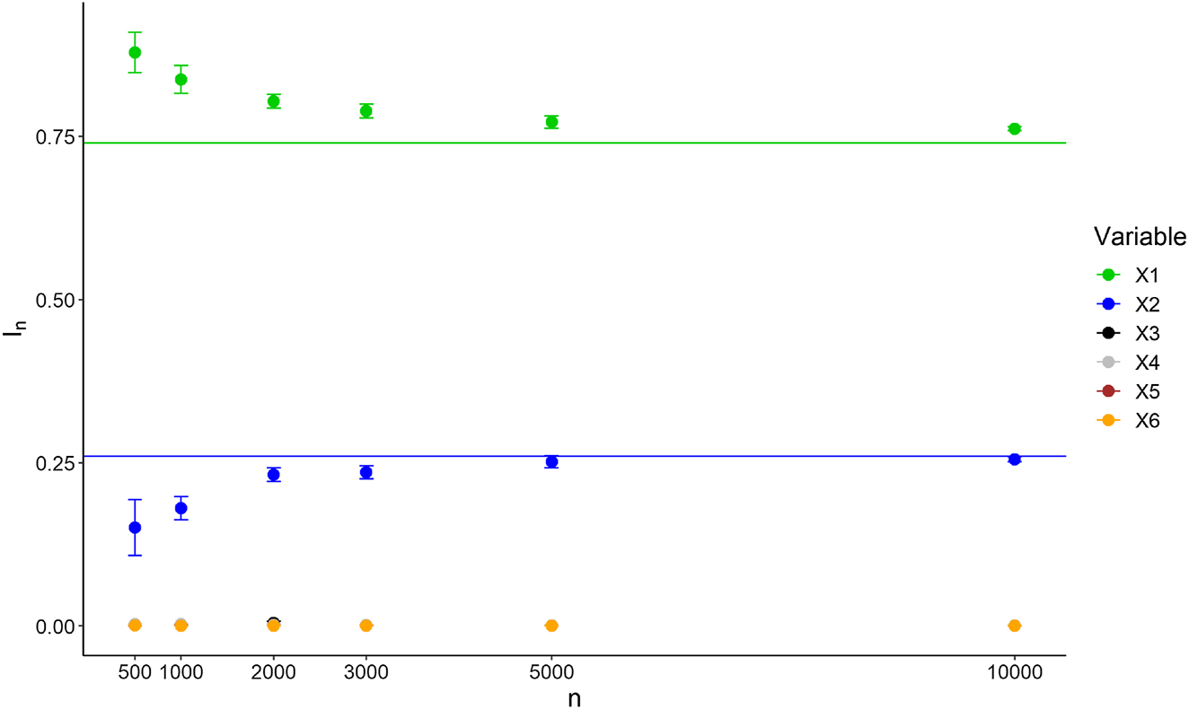
4.1.1 Experiment 1
We consider a first example of simulated data to highlight the good performance of the proposed importance measure. The input is a Gaussian vector of dimension p = 8, defined by
where
Variable importance of Experiment 1 for
| I | I n | TE-VIM | grf-vimp | ||||
|---|---|---|---|---|---|---|---|
| X (1) | 0.74 | X (1) | 0.77 (0.01) | X (1) | 0.74 (0.02) | X (1) | 0.70 (0.003) |
| X (2) | 0.26 | X (2) | 0.25 (0.01) | X (2) | 0.28 (0.01) | X (2) | 0.19 (0.003) |
| X (3) | 0 | X (3) | 0.001 | X (3) | 0.007 | X (3) | 0.03 |
| X (4) | 0 | X (4) | 0.001 | X (4) | −0.005 | X (4) | 0.03 |
| X (5) | 0 | X (5) | 0.0005 | X (5) | 0.003 | X (5) | 0.01 |
| X (6) | 0 | X (6) | 0.0003 | X (6) | 0.003 | X (6) | 0.01 |
| X (7) | 0 | X (7) | 0.0003 | X (7) | 0.003 | X (7) | 0.01 |
| X (8) | 0 | X (8) | 0.0003 | X (8) | 0.003 | X (8) | 0.01 |
Importance values
Variable importance of Experiment 1 with the dimension p set to 40 by adding noisy variables, for
| I | I n | TE-VIM | grf-vimp | ||||
|---|---|---|---|---|---|---|---|
| X (1) | 0.74 | X (1) | 0.79 (0.01) | X (1) | 0.80 (0.01) | X (1) | 0.56 (0.004) |
| X (2) | 0.26 | X (2) | 0.22 (0.01) | X (2) | 0.24 (0.01) | X (2) | 0.23 (0.003) |
| X (3) | 0 | X (3) | 0.001 | X (3) | −0.04 (0.01) | X (3) | 0.03 (0.002) |
| X (4) | 0 | X (4) | 0.001 | X (4) | −0.02 (0.01) | X (4) | 0.03 (0.003) |
| X (5) | 0 | X (5) | 0.00004 | X (5) | −0.02 (0.004) | X (5) | 0.004 |
| X (6) | 0 | X (6) | 0.00003 | X (6) | −0.01 (0.003) | X (6) | 0.005 |
| X (7) | 0 | X (7) | 0.00003 | X (7) | −0.01 (0.005) | X (7) | 0.004 |
| X (8) | 0 | X (8) | 0.00002 | X (8) | −0.01 (0.004) | X (8) | 0.005 |
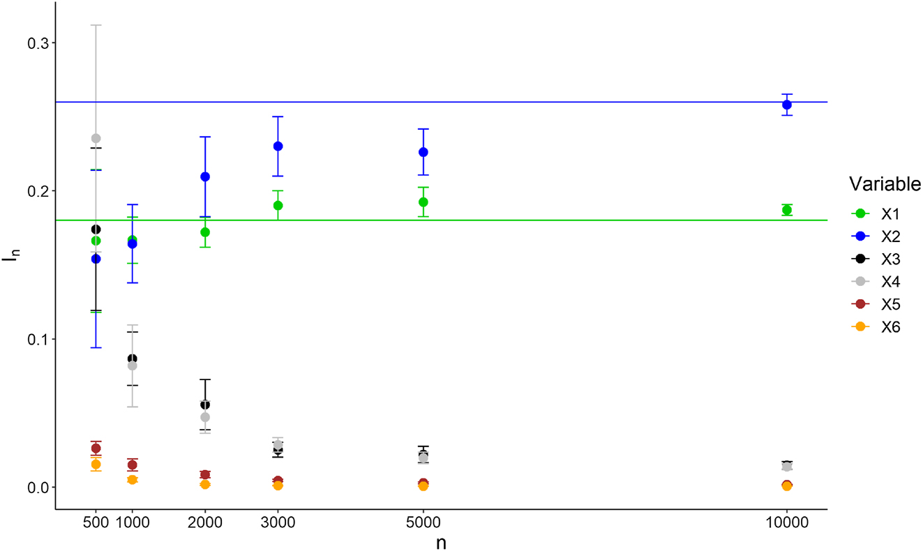
4.1.2 Experiment 2
We consider the same settings as in Experiment 1 with the original dimension p = 8, but we introduce three modifications to make the problem more difficult. In particular, we set
where
Variable importance ranking of Experiment 2 for
| I | I n | TE-VIM | grf-vimp | ||||
|---|---|---|---|---|---|---|---|
| X (2) | 0.26 | X (2) | 0.21 (0.008) | X (2) | 0.25 (0.06) | X (1) | 0.49 (0.01) |
| X (1) | 0.18 | X (1) | 0.19 (0.004) | X (1) | 0.13 (0.07) | X (4) | 0.12 (0.006) |
| X (3) | 0 | X (4) | 0.03 (0.005) | X (6) | −0.22 (0.14) | X (5) | 0.12 (0.007) |
| X (4) | 0 | X (3) | 0.03 (0.003) | X (8) | −0.23 (0.15) | X (2) | 0.11 (0.005) |
| X (5) | 0 | X (5) | 0.005 | X (5) | −0.24 (0.15) | X (3) | 0.11 (0.005) |
| X (6) | 0 | X (6) | 0.001 | X (7) | −0.28 (0.16) | X (7) | 0.02 (0.001) |
| X (7) | 0 | X (7) | 0.001 | X (3) | −0.32 (0.28) | X (8) | 0.02 (0.001) |
| X (8) | 0 | X (8) | 0.001 | X (4) | −0.55 (0.32) | X (6) | 0.02 |
The results displayed in Table 3 show that both our algorithm and TE-VIM provide the accurate variable ranking, where X
(2) is the most important variable, and X
(1) the second most important one. However, the standard deviations of the mean importance values over 50 repetitions are higher for TE-VIM, which is induced by a high instability across repetitions. This can be a limitation in practice with real data, as importance values are computed only once. We also observe that variables with a theoretical null importance get a quite strong negative bias. On the other hand, the importance measure from the grf package underestimates the importance of variable X
(2), and identifies X
(3), X
(4), and X
(5) as slightly more important than X
(2), although these three variables are not involved in the treatment heterogeneity by construction. In particular, X
(5) is not involved at all in the response Y, but is strongly correlated to the influential input X
(1). Because of this dependence, X
(5) is frequently used in the causal forests splits, leading to this quite high importance given by the grf package. On the other hand,
Importance values
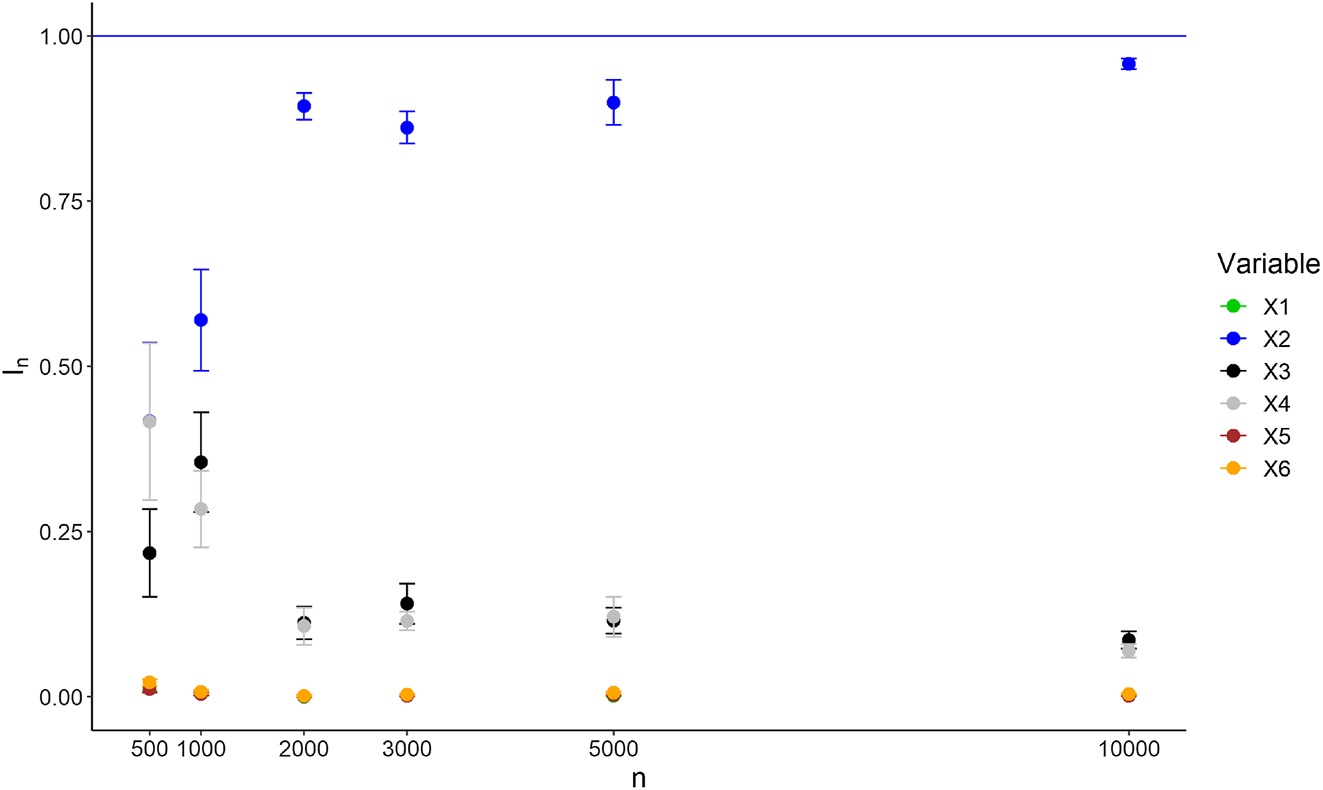
4.1.3 Experiment 3
This third experiment has the same setting than Experiment 2, except that variable X (1) is only a confounder and is not involved in the treatment effect heterogeneity anymore. Now, the response writes
The results are provided in Table 4. Clearly,
Variable importance ranking of Experiment 3 for
| I | I n | TE-VIM | grf-vimp | ||||
|---|---|---|---|---|---|---|---|
| X (2) | 1 | X (2) | 0.84 (0.02) | X (2) | 1.12 (0.6) | X (2) | 0.36 (0.01) |
| X (1) | 0 | X (4) | 0.16 (0.02) | X (3) | 0.63 (0.4) | X (4) | 0.24 (0.008) |
| X (3) | 0 | X (3) | 0.15 (0.02) | X (4) | 0.37 (0.2) | X (3) | 0.23 (0.008) |
| X (4) | 0 | X (7) | 0.007 (0.001) | X (1) | 0.29 (0.2) | X (6) | 0.04 (0.003) |
| X (5) | 0 | X (6) | 0.005 | X (8) | 0.29 (0.2) | X (8) | 0.04 (0.004) |
| X (6) | 0 | X (8) | 0.005 | X (7) | 0.29 (0.2) | X (7) | 0.04 (0.002) |
| X (7) | 0 | X (5) | 0.003 | X (5) | 0.25 (0.2) | X (1) | 0.03 (0.002) |
| X (8) | 0 | X (1) | 0.002 | X (6) | 0.17 (0.1) | X (5) | 0.03 (0.002) |
Importance values
4.1.4 Experiment 4
The goal of this fourth simulated experiment is to highlight a case where the corrective term in the retrained causal forest has a strong influence, as opposed to Experiments 1, 2, and 3. We consider p = 5 inputs uniformly distributed over [0,1], except X
(1) defined as X
(1) = U
3, where
where
Variable importance ranking of Experiment 4 for
| I n |
|
||
|---|---|---|---|
| X (1) | 0.98 (0.002) | X (1) | 1.57 (0.01) |
| X (2) | 0.0003 | X (2) | 0.001 |
| X (3) | 0.001 | X (3) | 0.001 |
| X (4) | 0.0002 | X (4) | 0.002 |
| X (5) | 0.0002 | X (5) | 0.001 |
4.2 ACIC Data Challenge 2019
We run a second batch of experiments using the data from the ACIC data challenge 2019 (https://sites.google.com/view/acic2019datachallenge/data-challenge), where the goal was to estimate ATEs in various settings. The input data is taken from real datasets available online on the UCI repository. Next, outcomes are simulated with different scenarios, and the associated code scripts were released after the challenge. Since the data generating mechanism is available, we have access to the variables involved in the heterogeneous treatment effect. In each scenario, a hundred datasets were randomly sampled.
We first use the “student performance 2” data with 29 input variables, considering Scenario 4 defined in the ACIC challenge, involving heterogeneity of the treatment effect with respect to X
(3). Each dataset is of size n = 649, and we run 50 repetitions with independent datasets for uncertainties. Table 6 gives the top 5 variables ranked by
Top 5 variables for “Student performance 2 (Scenario 4)” dataset using
|
|
TE-VIM | grf-vimp | |||
|---|---|---|---|---|---|
| X (3) | 0.85 (0.02) | X (3) | 0.82 (1.1) | X (3) | 0.44 (0.01) |
| X (29) | 0.013 (0.006) | X (26) | 0.22 (0.6) | X (29) | 0.06 (0.004) |
| X (28) | 0.007 (0.002) | X (20) | 0.06 (0.5) | X (28) | 0.04 (0.002) |
| X (27) | 0.006 (0.003) | X (25) | −0.09 (0.8) | X (25) | 0.04 (0.003) |
| X (25) | 0.005 (0.002) | X (19) | −0.25 (0.3) | X (27) | 0.03 (0.003) |
Secondly, we use the “spam email” data, made of 22 input variables. We also consider Scenario 4, where variables X
(8) and X
(19) are involved in the heterogeneous treatment effect. In this case, we merge 20 datasets to get a quite large sample of size n = 10000, and run 5 repetitions to compute standard deviations. The two relevant variables are properly identified as the most important ones by
Top 6 variables for “Spam email (Scenario 4)” dataset using
| I n | TE-VIM | grf-vimp | |||
|---|---|---|---|---|---|
| X (8) | 0.83 (0.001) | X (8) | 0.88 (0.01) | X (8) | 0.85 (4.10−3) |
| X (19) | 0.011 (0.002) | X (1) | 0.04 (0.007) | X (19) | 0.064 (6.10−3) |
| X (22) | 0.003 (4.10−4) | X (19) | 0.04 (0.007) | X (1) | 0.013 (3.10−3) |
| X (12) | 0.002 (4.10−4) | X (11) | 0.006 (0.007) | X (22) | 0.013 (1.10−3) |
| X (15) | 0.001 (3.10−4) | X (14) | 0.006 (0.006) | X (15) | 0.010 (8.10−4) |
| X (17) | 0.0004 (<10−4) | X (3) | 0.005 (0.006) | X (17) | 0.009 (2.10−3) |
4.3 Real data
4.3.1 Welfare data
For a first experiment with real data, we use the “Welfare” dataset from a GSS survey, introduced in Green and Kern [28] and available at https://github.com/gsbDBI/ExperimentData. The goal of this survey is to analyze the impact of question wording about the support of Americans to the government welfare spending. Respondents are randomly assigned one of two possible questions, with the same introduction and response options, but using the phrasing “welfare” or “assistance to the poor”. In fact, this slight wording difference has a quite strong impact on the survey answers, and defines the treatment. The output of interest indicates if respondents have answered that “too much” is spent. Our objective is to identify the main characteristics of individuals that have an impact on the heterogeneity of the treatment effect. The considered dataset is of size n = 13198 with p = 31 input variables, and basic data preparation steps were used to drop rows with missing values. Notice that imputing missing values may improve estimates. We leave this topic for future work, as handling missing values for variable importance is of high practical interest.
Table 8 displays the top 10 most important variables for Welfare data using our algorithm I n and also the importance from the grf package. The ranking provided by the two algorithms are close, but I n has a clear meaning as the variance proportion of the treatment effect lost when a given variable is removed, whereas grf-vimp can only be used as a relative importance between covariates, without an intrinsic meaning.
Top 10 most important variables with respect to I n and grf-vimp for Welfare data.
| I n | grf-vimp | ||
|---|---|---|---|
| polviews | 0.18 | polviews | 0.31 |
| partyid | 0.09 | partyid | 0.17 |
| hrs1 | 0.04 | educ | 0.09 |
| indus80 | 0.03 | indus80 | 0.07 |
| maeduc | 0.02 | hrs1 | 0.07 |
| educ | 0.02 | marital | 0.04 |
| marital | 0.01 | degree | 0.04 |
| age | 0.01 | maeduc | 0.04 |
| occ80 | 0.01 | occ80 | 0.02 |
| reg16 | 0.01 | age | 0.02 |
Notice that the sum of the importance of all input variables, i.e.
Group variable importance for Welfare data.
| Variable group |
|
|---|---|
| partyid, polviews | 0.51 |
| educ, sibs, occ80, prestg80, maeduc, degree | 0.23 |
| hrs1, income, rincome, wrkstat | 0.07 |
| age, marital, childs, babies | 0.04 |
| wrkslf, indus80, sex | 0.03 |
| reg16, mobile16 | 0.01 |
| race, res16, parborn, born | 0.00 |
| family16 | 0.00 |
| earnrs, hompop, adults | 0.00 |
| preteen, teens | 0.00 |
4.3.2 NHEFS health data
For the second case study, we use the NHEFS real data about body weight gain following a smoking cessation, extensively described in the causal inference book of Hernan and Robins [29]. As highlighted in the introduction of Chapter 12, these data help to answer the question “what is the average causal effect of smoking cessation on body weight gain?”. According to the authors, the unconfoundedness assumption holds. Here, we go a step further to analyze the heterogeneity of this causal effect with respect to health and personal data of individuals who have stopped smoking, using causal forests and our variable importance algorithm. The data record the weight of individuals, first measured in 1971, and then in 1982. The treatment assignment W indicates whether people have stopped smoking during this period, and the observed output Y is the weight difference between 1971 and 1982. We take the dataset of size n = 1566 used in Hernan and Robins [29, Chapter 12]. Notice that 63 rows with the output missing were removed, introducing a small bias, as discussed by the authors. They include 9 variables in their analysis, sufficient for unconfoundedness. To better estimate heterogeneity, we also include all variables of the original dataset, that do not contain missing values and are not related to the response, and obtain p = 41 input variables. As already mentioned, handling missing values is out of scope of this article, and is left for future work. We run our variable importance algorithm and the grf importance, using M = 4000 trees.
The results are displayed in Table 10. Clearly, the original weight of individuals in 1971 has a strong causal effect on weight gain following smoking cessation, with half of the treatment effect variance lost when this variable is removed. The intensity and duration of smoking, as well as personal characteristics, such as height and age are also involved in treatment heterogeneity, according to both algorithms. Notice that grf-vimp underestimates the importance of wt71 with respect to other variables. Next, we group together variables that are highly correlated, to compute group variable importance. We use the same clustering procedure as the Welfare case, except that we increase the number of groups to 30, since most variables have a very weak dependence with the others. Sex, height, and birth control are highly correlated with the weight in 1971, and this group explains two third of the treatment effect heterogeneity. In fact, age and smoke years also have a quite strong impact with a quarter of heterogeneity explained. Also notice that sex and birth control belong to the most influential group, but have a low importance
Top 10 most important variables with respect to I n and grf-vimp for NHEFS data.
| I n | grf-vimp | ||
|---|---|---|---|
| wt71 | 0.52 | wt71 | 0.26 |
| smokeyrs | 0.09 | smokeyrs | 0.13 |
| smokeintensity | 0.07 | age | 0.10 |
| ht | 0.06 | ht | 0.10 |
| age | 0.05 | smokeintensity | 0.07 |
| alcoholfreq | 0.01 | school | 0.07 |
| active | 0.01 | active | 0.03 |
| tumor | 0.01 | alcoholfreq | 0.03 |
| asthma | 0.01 | chroniccough | 0.02 |
| alcoholtype | 0.01 | marital | 0.02 |
Group variable importance for NHEFS data.
| Variable group |
|
|---|---|
| sex, ht, wt71, birthcontrol | 0.67 |
| age, smokeyrs | 0.26 |
| school, education | 0.03 |
| alcoholpy, alcoholfreq, alcoholtype | 0.02 |
| hbp, diabetes, pica, hbpmed, boweltrouble | 0.02 |
5 Conclusions
We introduced a new variable importance algorithm for causal forests, based on the drop and relearn principle, widely used for regression problems. The proposed method has both theoretical and empirical solid groundings. Indeed, we show that our algorithm is consistent, under standard assumptions in the mathematical analysis of random forests. Additionally, we run extensive experiments on simulated, semi-synthetic, and real data, to show the practical efficiency of the method. Notice that the implementation of our variable importance algorithm is available online at https://gitlab.com/random-forests/vimp-causal-forests.
Let us summarize the main guidelines for practitioners using our variable importance algorithm. First, all confounders must be included in the initial data, as it is always necessary to fulfill the unconfoundedness assumption to obtain consistent estimates. Secondly, it is also recommended to include all variables impacting heterogeneity in the data as well. However, leaving aside a non-confounding variable impacting heterogeneity, does not bias the analysis, as opposed to a missing confounder. Thirdly, practitioners must also keep in mind that adding a large number of irrelevant variables, i.e. non-confounding and not impacting heterogeneity, may hurt the accuracy of causal forests. Finally, it is recommended to group correlated variables together, and then compute group variable importance to get additional relevant insights.
We only consider binary treatment assignments throughout the article for the sake of clarity, but notice that the extension to conditional average partial effects with continuous treatment assignments is straightforward, since causal forests natively handle continuous assignments [6]. In this case, the outcome and treatment effect are directly defined through Equation (1) as
To conclude, we highlight two further research directions of interest. First, handling missing values in variable importance algorithms is barely discussed in the literature, but is strongly useful in practice, since observational databases often have missing values, which should be handled carefully to avoid misleading results. Secondly, developing a testing procedure to detect significantly non-null importance values, would enable to identify the set
-
Research funding: Julie Josse is supported in part by the French National Research Agency ANR16-IDEX-0006.
-
Author contributions: All authors have accepted responsibility for the entire content of this manuscript and consented to its submission to the journal, reviewed all the results and approved the final version of the manuscript.
-
Conflict of interest: Authors state no conflict of interest.
-
Data availability: The datasets from the ACIC data challenge 2019 are available at https://sites.google.com/view/acic2019datachallenge/data-challenge. The “Welfare” dataset is available at https://github.com/gsbDBI/ExperimentData. The NHEFS dataset is available at https://miguelhernan.org/whatifbook.
A Proofs of Propositions 1–5 and Theorems 1–5
Proof of Proposition 1.
Using the observed outcome definition with SUTVA (line 1), and the unconfoundedness Assumption 1 (line 2 to 3), we have
and the final result follows. □
Proof of Proposition 2.
From Assumption 2, X admits a strictly positive density, denoted by f. Then, from Definition 2,
which is strictly positive, since f is strictly positive and
Proof of Proposition 3.
Assumption 2 implies that
which also writes using the law of total variance
If
We now consider the case where
Proof of Proposition 4.
We first expand the covariance term
Notice that the second term is null since
then
which gives the final local moment equation in
Proof of Proposition 5.
As in the proof of Proposition 4, we obtain
Notice that
Combining the above two equations, we have
which gives the final result since
□
Proof of Theorem 1.
The result is obtained by applying Theorem 3 from Athey et al. [6]. The first paragraph of Section 3 of Athey et al. [6] provides conditions to apply Theorem 3, that are satisfied by our Assumptions 3 and 4: X ∈ [0,1] p , X admits a density bounded from below and above by strictly positive constants, and μ and τ are bounded.
Next, Assumptions 1–6 from Athey et al. [6] must be verified. As stated at the end of Section 6.1, Assumptions 3–6 always hold for causal forests, the first assumption holds because the functions m, μ, and τ are Lispschitz from our Assumption 4 (the product of Lipschitz functions is Lipschitz), and Assumption 2 is satisfied because
Finally, the forest is grown from Specification 1, and the treatment effect is identified by Equation (3) since Assumption 1 enforces unconfoundedness. Overall, we apply Theorem 3 from Athey et al. [6] to get the consistency of the causal forest estimate, i.e., for x ∈ [0,1] p
Notice that Theorem 3 from Athey et al. [6] states the consistency of generalized forests. As it will be useful for further results, we give below a proof of the weak consistency in the specific case of causal forests, using arguments of Athey et al. [6]. In particular, we take advantage of Specification 1, which enforces the honesty property, and that the diameters of tree cells vanish as the sample size n increases. First, in our case of binary treatment W, the causal forest estimate writes
where the weight α
i
(x) is defined by Equation (3) of Athey et al. [6], as the weight associated to training observation X
i
to form an estimate at the new query point x. The weights α
i
(x) sum to 1 over all observations, i.e.,
and then,
Here, we use a key property of the forest growing given by Specification 1: honesty. Indeed, it enforces that
Since W and Y are independent conditional on X from the unconfoundedness Assumption 1,
Since Assumptions 3 and 4 and Specification 1 are satisfied, Equation (26) in the Supplementary Material of Athey et al. [6] states that
which gives that
Next, we use Equation (24) in Lemma 7 of the Supplementary Material of Athey et al. [6], to get that
Identically, we obtain the weak consistency of the other terms involved in τ
M,n
(x), i.e.,
where the last line is given by the local moment Equation (3), which identifies the treatment effect. Finally, notice that this proof applies to any linear local moment equation defining a generalized random forest. □
Proof of Theorem 2.
We consider
where θ(x (−j)) satisfies the following equation by definition of causal forests,
Then, according to Proposition 4, the above moment equation identifies the treatment effect under Assumptions 1 and 2, and we obtain
which gives (i). For (ii), we apply the same proof, except that the obtained local moment equation identifies
Proof of Theorem 3.
With j ∈ {1, …, p}, recall that the causal forest τ
M,n
(x) is fit with a centered dataset
where
Using the same proof as for Theorem 1, we get that
For the second term involved in Δ
n
, we cannot directly apply the proof of Theorem 1 since the output depends on n through the term τ
M,n
(X
i
). We first need to bound
where t
0 is the maximum number of observations in each terminal leave. Since the weights are identically distributed, we have
Next, for the second term of Δ n , we write
The right hand side of this inequality writes
where the last inequality is obtained using (13). Finally, since the original causal forest trained with all inputs and the weights
Since Theorem 1 gives the convergence in probability towards 0 of τ
M,n
(x) − τ(x) for all x ∈ [0, 1] and Z
n
is independent from τ
M,n
(x), we get that
This implies the convergence of the second term of Δ n , and overall, we obtain that
Next,
Then, following the case (ii) of Theorem 2, we get
which gives the final result
where the last equality is given by Proposition 5. □
Proof of Theorem 4.
We first consider the case
According to Specification 2,
Next, recall that
We first consider
and then
Since |Δ n,1| = Δ n,1, according to Equation (14), we have
which also implies the convergence in probability of Δ n,1.
Similarly for the denominator, we write
We first show the convergence of
where the limit is obtained because Theorem 1 gives the weak consistency of τ
M,n
(X), which implies the convergence of the first moment since τ
M,n
(X) is bounded from Specification 2. Next, we show that the variance of
For
since τ
M,n
(X) is bounded by K from Specification 2. We thus obtain
where this upper bound converges to 0, since τ
M,n
(X) converges towards
Using the continuous mapping theorem, we conduct the same analysis to get that
with
and following the same arguments, we get that
Proof of Theorem 5.
We can directly deduce from the proof of Theorem 3 that, for x ∈ (0, 1),
We denote by C
j
(x
(−j)) the second term of the above limit to lighten notations. Next, we follow the proof of Theorem 4 to get the convergence of
The numerator writes
Then, we have
which gives the final result. □
References
1. Obermeyer, Z, Emanuel, EJ. Predicting the future–big data, machine learning, and clinical medicine. N Engl J Med 2016;375:1216–19. https://doi.org/10.1056/nejmp1606181.Search in Google Scholar PubMed PubMed Central
2. Kennedy, EH. Towards optimal doubly robust estimation of heterogeneous causal effects. Electronic J. Statistics 2023;17:3008–49. https://doi.org/10.1214/23-ejs2157.Search in Google Scholar
3. Nie, X, Wager, S. Quasi-oracle estimation of heterogeneous treatment effects. Biometrika 2021;108:299–319. https://doi.org/10.1093/biomet/asaa076.Search in Google Scholar
4. Künzel, S, Sekhon, JS, Bickel, PJ, Yu, B. Metalearners for estimating heterogeneous treatment effects using machine learning. Proc Natl Acad Sci 116; 2019. p. 4156–65. https://doi.org/10.1073/pnas.1804597116.Search in Google Scholar PubMed PubMed Central
5. Wager, S, Athey, S. Estimation and inference of heterogeneous treatment effects using random forests. J Am Stat Assoc 2018;113:1228–42. https://doi.org/10.1080/01621459.2017.1319839.Search in Google Scholar
6. Athey, S, Tibshirani, J, Wager, S. Generalized random forests. Ann Stat 2019;47:1148–78. https://doi.org/10.1214/18-aos1709.Search in Google Scholar
7. Kosuke, I, Marc, R. Estimating treatment effect heterogeneity in randomized program evaluation. Ann Appl Stat 2013;7:443–70. https://doi.org/10.1214/12-aoas593.Search in Google Scholar
8. Hill, JL. Bayesian nonparametric modeling for causal inference. J Comput Graph Stat 2011;20:217–40. https://doi.org/10.1198/jcgs.2010.08162.Search in Google Scholar
9. Shalit, U, Johansson, FD, Sontag, D. Estimating individual treatment effect: generalization bounds and algorithms. In International Conference on Machine Learning. PMLR; 2017:3076–85 pp.Search in Google Scholar
10. Zhao, Y, Zeng, D, Rush, AJ, Kosorok, MR. Estimating individualized treatment rules using outcome weighted learning. J Am Stat Assoc 2012;107:1106–18. https://doi.org/10.1080/01621459.2012.695674.Search in Google Scholar PubMed PubMed Central
11. Swaminathan, A, Joachims, T. Batch learning from logged bandit feedback through counterfactual risk minimization. J Mach Learn Res 2015;16:1731–55.Search in Google Scholar
12. Kitagawa, T, Tetenov, A. Who should be treated? Empirical welfare maximization methods for treatment choice. Econometrica 2018;86:591–616. https://doi.org/10.3982/ecta13288.Search in Google Scholar
13. Athey, S, Wager, S. Policy learning with observational data. Econometrica 2021;89:133–61. https://doi.org/10.3982/ecta15732.Search in Google Scholar
14. Tibshirani, J, Athey, S, Sverdrup, E, Wager, S. grf: Generalized Random Forests. R package version 2.3.0 2023. https://CRAN.R-project.org/package=grf.Search in Google Scholar
15. Hines, O, Diaz-Ordaz, K, Vansteelandt, S. Variable importance measures for heterogeneous causal effects. arXiv preprint arXiv:2204.06030 2022.Search in Google Scholar
16. Boileau, P, Qi, NT, Van Der Laan, MJ, Dudoit, S, Leng, N. A flexible approach for predictive biomarker discovery. Biostatistics 2023;24:1085–105. https://doi.org/10.1093/biostatistics/kxac029.Search in Google Scholar PubMed
17. Lei, J, G’Sell, M, Rinaldo, A, Tibshirani, RJ, Wasserman, L. Distribution-free predictive inference for regression. J Am Stat Assoc 2018;113:1094–111. https://doi.org/10.1080/01621459.2017.1307116.Search in Google Scholar
18. Williamson, BD, Gilbert, PB, Simon, NR, Carone, M. A general framework for inference on algorithm-agnostic variable importance. J Am Stat Assoc 2023;118:1645–58. https://doi.org/10.1080/01621459.2021.2003200.Search in Google Scholar PubMed PubMed Central
19. Hooker, G, Mentch, L, Zhou, S. Unrestricted permutation forces extrapolation: variable importance requires at least one more model, or there is no free variable importance. Stat Comput 2021;31:1–16. https://doi.org/10.1007/s11222-021-10057-z.Search in Google Scholar
20. Bénard, C, Da Veiga, S, Scornet, E. Mean decrease accuracy for random forests: inconsistency, and a practical solution via the Sobol-MDA. Biometrika 2022;109:881–900. https://doi.org/10.1093/biomet/asac017.Search in Google Scholar
21. VanderWeele, TJ, Robins, JM. Four types of effect modification: a classification based on directed acyclic graphs. Epidemiology 2007;18:561–8. https://doi.org/10.1097/ede.0b013e318127181b.Search in Google Scholar
22. Rothman, KJ. Epidemiology: an introduction. Oxford University Press; 2012.Search in Google Scholar
23. Colnet, B, Josse, J, Varoquaux, G, Scornet, E. Risk ratio, odds ratio, risk difference…which causal measure is easier to generalize? arXiv preprint arXiv:2303.16008 2023.Search in Google Scholar
24. Sobol, IM. Sensitivity estimates for nonlinear mathematical models. Math Model Comput Experiments 1993;1:407–14.Search in Google Scholar
25. Athey, S, Wager, S. Estimating treatment effects with causal forests: an application. Observational Studies 2019;5:37–51. https://doi.org/10.1353/obs.2019.0001.Search in Google Scholar
26. Meinshausen, N. Quantile regression forests. J Mach Learn Res 2006;7:983–99.Search in Google Scholar
27. Scornet, E, Biau, G, Vert, J-P. Consistency of random forests. Ann Stat 2015;43:1716–41. https://doi.org/10.1214/15-aos1321.Search in Google Scholar
28. Green, DP, Kern, HL. Modeling Heterogeneous treatment effects in survey experiments with bayesian additive regression trees. Public Opin Q 2012;76:491–511. https://doi.org/10.1093/poq/nfs036.Search in Google Scholar
29. Hernan, MA, Robins, J. Causal inference: what if. Boca Raton: Chapman & Hall/CRC; 2020.Search in Google Scholar
© 2025 the author(s), published by De Gruyter, Berlin/Boston
This work is licensed under the Creative Commons Attribution 4.0 International License.
Articles in the same Issue
- Research Articles
- Decision making, symmetry and structure: Justifying causal interventions
- Targeted maximum likelihood based estimation for longitudinal mediation analysis
- Optimal precision of coarse structural nested mean models to estimate the effect of initiating ART in early and acute HIV infection
- Targeting mediating mechanisms of social disparities with an interventional effects framework, applied to the gender pay gap in Western Germany
- Role of placebo samples in observational studies
- Combining observational and experimental data for causal inference considering data privacy
- Recovery and inference of causal effects with sequential adjustment for confounding and attrition
- Conservative inference for counterfactuals
- Treatment effect estimation with observational network data using machine learning
- Causal structure learning in directed, possibly cyclic, graphical models
- Mediated probabilities of causation
- Beyond conditional averages: Estimating the individual causal effect distribution
- Matching estimators of causal effects in clustered observational studies
- Ancestor regression in structural vector autoregressive models
- Single proxy synthetic control
- Bounds on the fixed effects estimand in the presence of heterogeneous assignment propensities
- Minimax rates and adaptivity in combining experimental and observational data
- Highly adaptive Lasso for estimation of heterogeneous treatment effects and treatment recommendation
- A clarification on the links between potential outcomes and do-interventions
- Valid causal inference with unobserved confounding in high-dimensional settings
- Spillover detection for donor selection in synthetic control models
- Causal additive models with smooth backfitting
- Experiment-selector cross-validated targeted maximum likelihood estimator for hybrid RCT-external data studies
- Applying the Causal Roadmap to longitudinal national registry data in Denmark: A case study of second-line diabetes medication and dementia
- Orthogonal prediction of counterfactual outcomes
- Variable importance for causal forests: breaking down the heterogeneity of treatment effects
- Multivariate zero-inflated causal model for regional mobility restriction effects on consumer spending
- Rate doubly robust estimation for weighted average treatment effects
- Adding covariates to bounds: what is the question?
- Review Article
- The necessity of construct and external validity for deductive causal inference