
Impact of domain knowledge on developing pumping models for single-screw extruders using symbolic regression
-
Daniel Herzog
 ,
Florian Lehner
,
Florian Lehner

Abstract
Reliable process models are a valuable asset in polymer extrusion to reduce downtimes and rejects, to improve process efficiency, and to accelerate the development of new screw designs. With ongoing progress in computational capabilities, increasing attention is paid to modeling techniques that infer predictions directly from the process data. Out of these, symbolic regression is an attractive option for process engineers, since it provides information as ready-to-use analytical mathematical expressions. However, extensive workload for data curation and model generation impedes obtaining regression models of high precision and general validity. In polymer extrusion, integrating domain knowledge into the regression data is already known to support the search for accurate prediction models. To assess this benefit systematically and quantitatively, we developed symbolic regression models for the pumping characteristics of single-screw extruders from three-dimensional fluid dynamics simulations, including different modules of domain knowledge at data preprocessing: Initially, models are created (i) using theory of similarity only, followed by models that further (ii) accept derived physical parameters as additional input features, (iii) combine additional input features with logarithmic scaling, and (iv) correct a theoretical approximation equation. For each case of data preprocessing, the regression models are evaluated in terms of their interpolation and extrapolation capabilities, their structural complexities, and their required training times. This study demonstrates that symbolic regression is most efficient on the original dimensionless data if nonlinear trends in dimensionless space remain below second order or within one decade. Once stronger nonlinearities occur, however, capturing these nonlinearities with prior theoretical approximations substantially enhances extrapolation capability and computational efficiency, albeit at the price of larger models.
Nomenclature
Symbol Parameter
- cos
-
cosine function
- D
-
inner barrel diameter
- e
-
axial flight width
- ETT
-
expected training time
- exp
-
natural exponential function
- h
-
channel depth
- h/w b
-
channel aspect ratio
- K
-
power-law consistency
- L
-
screw (segment) length
- ln
-
natural logarithm
-
-
mass flow rate
- MAE
-
mean absolute error
- n
-
power-law index
- N runs
-
number of runs (symbolic regressions)
- N disc
-
number of discarded models
- R 2
-
coefficient of determination
- sin
-
sine function
- t
-
screw pitch
- TT
-
training time
- w b
-
outer channel width
-
-
shear rate
- η
-
shear viscosity
- ΔΠ V
-
dimensionless flow rate residual
- Π p
-
dimensionless down-channel pressure gradient
- Π V
-
dimensionless flow rate
-
-
predicted dimensionless flow rate for design point i
- Π V,scaled
-
scaled dimensionless flow rate
-
-
simulated dimensionless flow rate for design point i
- φ b
-
outer pitch angle
- √
-
square root
1 Introduction
Extrusion is a key manufacturing process for the plastics, food, and pharmaceutical industries, being involved in at least one processing step along the value chain. Steadily growing demands on productivity, product quality and process efficiency fuel the need for mathematical models that predict extruder performance fast and reliably. Yet this performance is influenced by multiple complex and interlinked physical phenomena, which are difficult to capture altogether by purely analytical or numerical approaches. In the era of “big data” and continuous progress in computational power, data-based modeling techniques can overcome this challenge (Roland et al. 2022).
In the recent two decades, several data-based approaches have been applied to describe extrusion processes, including support vector machines (Chitralekha and Shah 2010), decision trees (Ronowicz et al. 2015), and artificial neural networks (Kowalski et al. 2021). Polychronopoulos et al. (2025) assessed the capabilities of these machine learning algorithms for predicting the process performance of single-screw extruders. Despite their high predictive potential, all these approaches are “blackboxes” with little insight into their internal behavior. Lack of transparency and interpretability may discourage the adoption of such black-box algorithms for extrusion engineering, where understanding the relations between design and process variables is important. Increasing and ongoing efforts are taken to gain more insight into the reasoning of classical machine learning algorithms. Examples are permutation feature importance, function decomposition, partial dependency plots, penalizing large structures of tree-based models, or testing neural networks on abstract concepts (Molnar 2020; Rudin et al. 2022).
Another attractive alternative is given by symbolic regression, as it provides interpretable analytical mathematical expressions to relate decision variables (Makke and Chawla 2024; Roland et al. 2021). Unlike traditional regression procedures, symbolic regression optimizes model structure and coefficients simultaneously, usually by means of genetic algorithms. This high flexibility allows for nonlinear and coupled effects to be captured even beyond the dataspace provided for model creation (Roland et al. 2021) without the need to know the underlying functional relationships a priori. The expressive power of symbolic regression is increasingly acknowledged in various scientific disciplines, such as materials science (Versino et al. 2017), earth science (Li et al. 2024), astronomy (Matchev et al. 2022), medicine (La Cava et al. 2023), and process engineering (Scheffold et al. 2021). In the field of polymer processing, symbolic regression has been successfully employed for modeling single-screw (Herzog et al. 2024) and twin-screw extruders (Stritzinger et al. 2023), melt filtration units (Pachner et al. 2021), multilayer die flow (Hammer et al. 2021), and shaping of corrugated pipes (Albrecht et al. 2022).
Without supporting information, however, symbolic regression tends to propose unphysical solutions, since model accuracy is optimized based on a finite set of elementary functions and training samples only. In general, such solutions will lead to poor predictions for unseen cases, especially in sparsely sampled subspaces and in the extrapolation regime. Simultaneously, genetic algorithms for symbolic regressions are computationally very expensive (Roland et al. 2021), while symbolic regressions based on neural networks can handle only a limited library of expressions (Makke and Chawla 2024). Hence, a sufficiently generalizable model can only be obtained at the price of laborious data collection and training, with possibly multiple rejections of useless models.
To compensate for the weaknesses of symbolic regression, several strategies have been devised to integrate domain knowledge into the model development process. One option involves considering shape constraints on the model functions, such as monotonicity, during model selection within the regression algorithm. These constraints can be strictly enforced, as investigated by Kronberger et al. (2022), or balanced against prediction accuracy, as proposed by Kubalík et al. (2020). As the constraints can be evaluated only approximately on a discrete number of samples, however, no supporting information for extrapolation is available, and dense data coverage with considerable computational overhead is required to minimize the portion of poorly interpolating models. Alternatively, domain knowledge can be provided to the regression algorithm at the stage of data preprocessing: Versino et al. (2017) introduced user-defined input features and artificial sample points from known solutions, while Zhou et al. (2023) combined user-defined features with logarithmic scaling of the targets. For single-screw extrusion modeling, Marschik et al. (2023) and Herzog et al. (2024) determined residuals of the target quantities with respect to theoretical approximations, and employed a classical genetic programming scheme to fit a symbolic expression to the residuals. All these data preprocessing strategies have proven to yield generally more accurate models across an extended design space. However, a comprehensive cost-benefit analysis of knowledge-based data preprocessing on symbolic regression modeling has not been performed to date, which compares and quantifies the impact of different knowledge modules.
This paper provides information on the numerical and statistical significance of domain knowledge for symbolic regression, taking simulated pressure-throughput characteristics for metering channels in single-screw extruders as use case. The main objective is to quantify the added value of knowledge-based data-preprocessing on both the obtained extrusion models and the model development process. Adding to the high cost-saving potential of generalized analytical equations compared to full-scale numerical simulations or experiments, the gained insights shall remove barriers for developing and implementing symbolic regression models for real-world engineering tasks. For this purpose, we start with describing the modeling task and the database in Section 2, followed by the strategies for knowledge integration and the regression analysis in Section 3. Section 4 is dedicated to the key results of the study. Based on these results, we finally give recommendations for model developers and applicants in industry and research.
2 Use case
This paper focuses on the melt conveying characteristics of single-flighted screw channels for two reasons: (i) they are practically relevant for most polymer processing operations, and (ii) they are already well studied (Campbell and Spalding 2013; Marschik et al. 2022; Rauwendaal 2014). These melt conveying characteristics link the local melt flow rate to the down-channel pressure gradient and serve as surrogate models for a segmented calculation of extruder performance, offering a quick alternative to full-scale three-dimensional simulations. For a given operating point, these models already allow conclusions on the standalone behavior of the melt conveying zone. The actual operating conditions in this zone, however, are affected by the conveying performance of the upstream zones, as well as by the flow resistance of the downstream shaping die. As most extruders are fed with solid material, at least four additional sub-processes need to be modeled alongside melt conveying to assess global extruder performance – (i) solids conveying, (ii) mixed-phase conveying, (iii) plastication, and (iv) die flow.
For deriving functional expressions for the melt conveying characteristics, symbolic regression is embedded in a hybrid modeling approach that combines analytical, numerical, and data-driven techniques, as illustrated in Figure 1: Initially, the extrusion process is analytically described as a mathematical problem of reasonable complexity, defining inputs and targets for the models and the governing equations behind the relevant physical phenomena. Next, the governing equations are solved numerically in an extensive parametric study to generate a representative database for all extrusion setups of interest. Finally, the numerical data points are approximated by continuous functions that can be implemented in extruder calculation routines, leveraging the expressive power of symbolic regression. Within this framework, domain knowledge is provided to the symbolic regression at two stages: (i) during the analytical problem formulation using theory of similarity, and (ii) optionally during data preprocessing. The hybrid modeling approach is applicable to any natural process or system that is fully described by continuous numerical data. It has been successfully employed to predict other polymer processing operations such as twin-screw extrusion, coextrusion die flow, and shaping of corrugated pipes. More detailed information on the hybrid modeling approach is given by Roland et al. (2022).
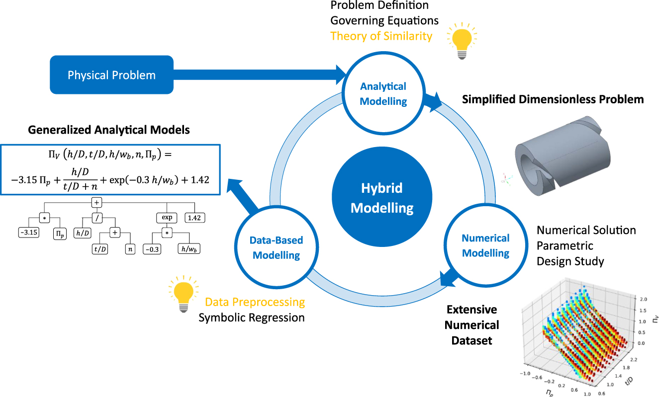
Hybrid modeling approach to derive generalized expressions for melt conveying characteristics in single-screw extruders. All steps that integrate domain knowledge in this study are highlighted in yellow.
2.1 Problem description
Applying domain knowledge to preprocess data on the use case investigated requires familiarity with the underlying physical principles. Figure 2 schematically illustrates the basic configuration of the melt conveying process in single-screw extruders: A helical screw segment with channel depth h, pitch t and axial flight width e is turning at angular speed ω inside a cylindrical barrel with inner diameter D. From these variables, the outer pitch angle φ b , outer channel width w b , and relative screw velocity v b at the barrel perimeter can be computed as
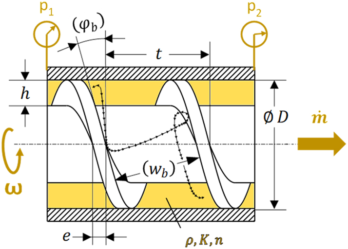
Basic configuration for the melt conveying process in a single-screw extruder.
While rotating, the active flight flank pushes the molten polymer forward at a certain mass flow rate
A full consideration of all influencing factors on the flow would create a high-dimensional design space. Since the required number of design points for good approximation models grows exponentially with the number of factors, the effort for both data generation and model creation quickly becomes unaffordable. Furthermore, the resulting regression model, if achievable, would be too complex for an efficient implementation in an extrusion calculation. For reasons of practical utility, the regression models are based on a (reasonably) simplified physical representation of the melt conveying process: The flow is assumed to be steady, isothermal and fully developed, with inertia and gravity effects being neglected. Furthermore, the clearance between the barrel and flight tip is ignored. The polymer melt is treated as an incompressible, inelastic, and wall-adhering fluid, and its shear thinning nature is considered by a power-law model that relates shear viscosity η and shear rate magnitude
Both the isothermal hypothesis and the omitted flight clearance do not match real extrusion processes and hence deserve further discussion. Indeed, as polymer melts are highly viscous and thermally insulating, pronounced temperature gradients may arise in the screw channel that affect the pumping capability via the temperature-dependent polymer properties. Moreover, the leakage across the screw flights notably diminishes the flow rate in pressure-generating zones and enhances the flow rate for strongly overridden zones. When relating the material properties to a mass-flow weighted mean temperature, however, transverse temperature gradients play a minor role, as convection is the main source of heat transfer in polymer extrusion (Potente et al. 2005). Down-channel temperature variations can be considered by subdividing the metering zone into sufficiently short segments with locally evaluated material properties (Roland et al. 2020). Two approaches are available to include the contribution of the leakage flow: (i) applying analytical correction factors on the linearized melt conveying characteristics (Tadmor and Klein 1970), or (ii) modeling the melt conveying zone as network of interconnected flow passages (Marschik et al. 2018). The remaining assumptions are justified for the majority of single-screw extrusion processes. More detailed information and a discussion on the physical modeling can be found in Marschik and Roland (2023b) and Herzog et al. (2024).
For developing the regression models, the governing equations of viscous fluid flow are further converted into dimensionless form using the theory of similarity. This procedure already integrates domain knowledge into the regression analysis by identifying the independent influencing parameters on the flow. In the language of machine learning, theory of similarity thus serves as a tool for feature selection. The major advantages are a reduced dimensionality of the data space, more uniform ranges of values for the variables, and more general models that cover similar processes at different scales. For the melt-conveying problem under consideration, the five independent influencing parameters (features) are according to Herzog et al. (2024):
the channel depth ratio h/D,
the screw pitch ratio t/D,
the axial flight width ratio e/D,
the power-law index n,
and the dimensionless down-channel pressure gradient
with p1 and p2 denoting the respective average pressures at the inlet and outlet of the screw segment according to Figure 2. This process parameter relates the pressure difference along the channel to the viscous stress under simple shear flow.
The target variable to be predicted is the dimensionless flow rate Π
V
of the extruder, which is the ratio of the observed mass throughput
2.2 Database
The database for this study consists of 21,069 numerical simulation results from Herzog et al. (2024) for the dimensionless flow rate Π V through metering screws with a fixed axial flight width ratio e/D = 0.1. The results for each design point were computed using the finite-volume method within the commercial software package ANSYS Fluent, version 2022R2 (Ansys Inc. 2022). A representative dimensional setup of D = 50 mm, K = 500 Pa sn and v b cos φ b = 1 m/s was specified to calculate the required input parameters for the solver using Equations (3)–(5) and to convert the obtained volumetric flow rate into dimensionless form using Equation (6). The simulations were performed in a rotating reference frame attached to the screw segment and with periodic boundary conditions at the open ends. On the mathematical level, a coupled solver with second-order interpolation was employed alongside a uniform hexahedral grid. Convergence was checked by tracking the standard deviation of the volumetric flow rate within the latest iterations. For details on the numerical solution process, the reader is referred to Herzog et al. (2024).
For an unbiased evaluation of the models, this database was partitioned into disjoint subsets for (i) model creation (training), (ii) interpolation, and (iii) extrapolation. The distribution of values in the respective datasets is highlighted in Figure 3. All datasets have fixed levels assigned to h/D, t/D and n, while the values for Π p were sampled continuously. For training and interpolation, an identical subspace was chosen that covers most conventional extrusion processes. The vertices of this subspace were exclusively reserved for training, while the remaining design points within the subspace were randomly assigned to the training and interpolation datasets. As a result, the data points for training and interpolation are almost evenly spread within their sub-range (the sharp peaks are related to the fixed levels for h/D, t/D and n). The extrapolation set spans the complete value range of the simulations outside the subspace for training and contains design points for high-performance extrusion. Though leaning towards higher h/D, smaller n and larger negative Π p , the levels of the interpolation range are still significantly represented and well-balanced in the extrapolation set (i.e., extrapolation is considered equally along all parameter axes). Moreover, the transition between the interpolation and extrapolation region is seamless in all dimensions. The sizes and value ranges of the datasets are additionally listed in Table 1. Although the polymer melt never flows backwards in the screw channel, samples with slightly negative flow rates (−0.1 < Π V < 0) were intentionally considered in this study to support the approximation of the dam-up pressure.
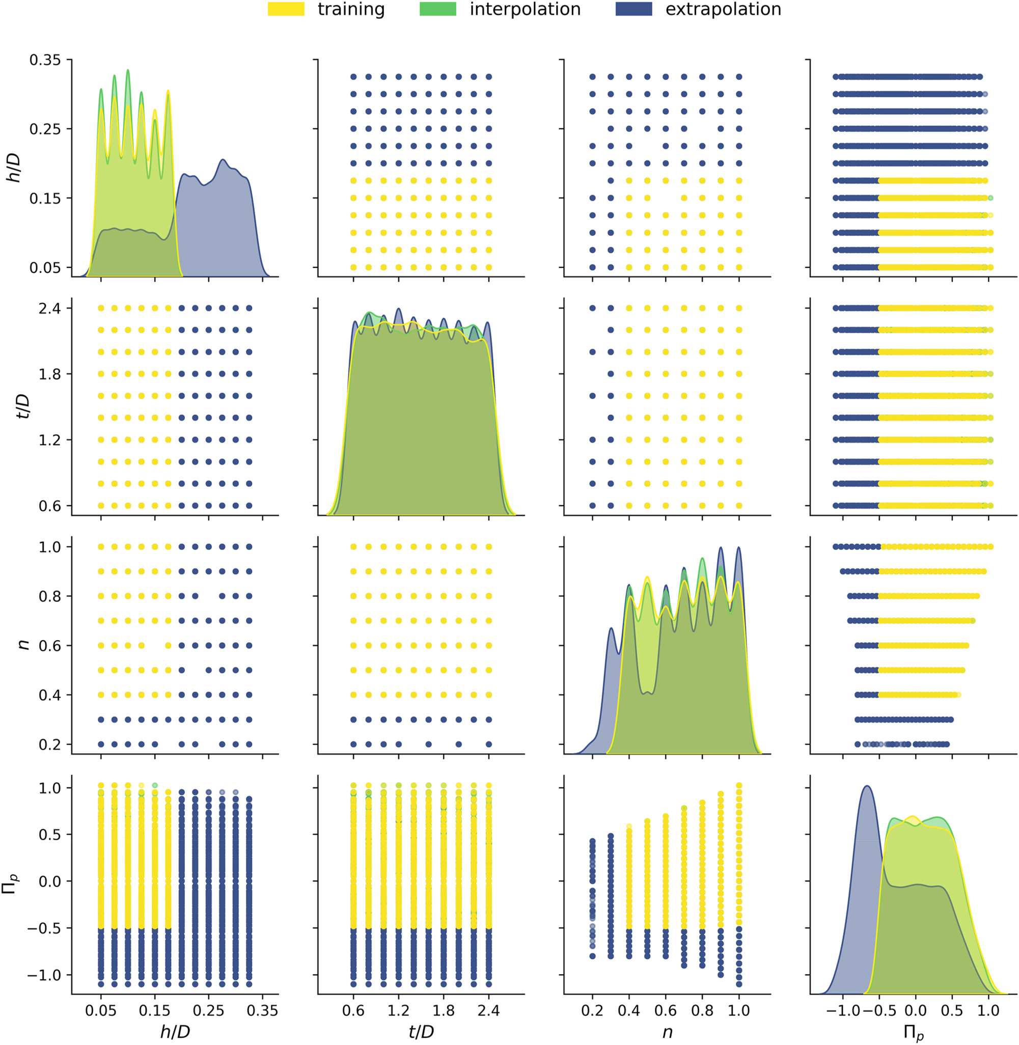
Distribution of values in the datasets for training (yellow), interpolation (green) and extrapolation (blue). The density plots along the diagonal show the relative frequency of values for each independent influencing parameter. The off-diagonal scatter plots indicate the pair-wise distribution of the parameter values.
Composition of the individual datasets.
| Dataset: | Train | Interpolation | Extrapolation |
|---|---|---|---|
| Design points | 3,026 | 4,223 | 13,820 |
| h/D range | [0.05; 0.175] | [0.05; 0.175] | [0.5; 0.325] |
| t/D range | [0.6; 2.4] | [0.6; 2.4] | [0.6; 2.4] |
| n range | [0.4; 1] | [0.4; 1] | [0.2; 1] |
| Π p range | [−0.5; 1.1] | [−0.5; 1.1] | [−1.1; 1.1] |
| Π V range | [−0.1; 2] | [−0.1; 2] | [−0.1; 15] |
To reveal inherent patterns in the data, Figure 4 highlights the dimensionless pressure-throughput relationship for two distinct extruder screw designs and various polymer melts. Two striking trends are evident: The dimensionless flow rate (i) monotonically decreases with the dimensionless down-channel pressure gradient Π p , and (ii) the characteristics become steeper and increasingly nonlinear at lower power-law indices n. For the lowest power-law index of 0.2, the dimensionless flow rate becomes highly sensitive on Π p , attaining values one decade above the more common range for interpolation (Table 1). As all simulations have been properly executed and are fully converged, these exceptional data points must be considered valid. For the limiting case of a flat and infinitely wide channel, Roland et al. (2019) also validated this behavior with an analytical approximation solution. This approximation solution follows a progressive power law in the limit of large Π p . A generally applicable regression model for single-screw extrusion should capture this asymptotic behavior and, simultaneously, closely predict more common extrusion settings. Mathematically speaking, a both well-interpolating and reasonably extrapolating model is required.
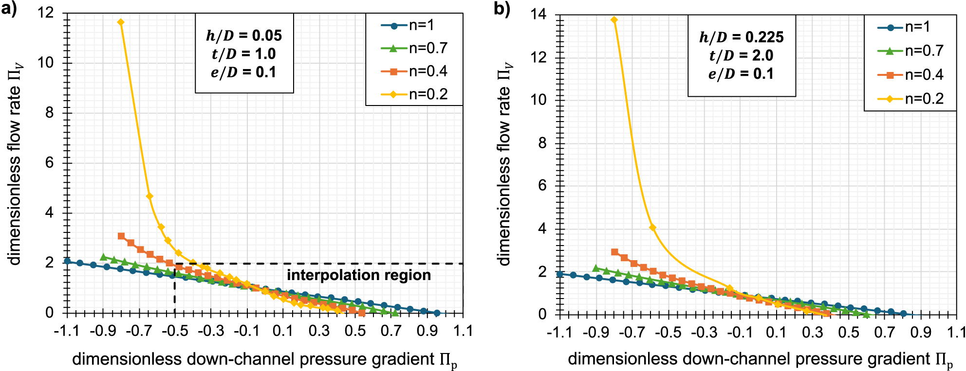
Exemplary dimensionless pressure-throughput characteristics for a conventional metering zone (a) and a high-performance screw design (b) for a wide range of power-law indices of the polymer melt. The boundary of the interpolation region is highlighted by the black dashed lines in (a). The curves only serve to better visualize the trends and do not represent a model fit.
3 Methodology
3.1 Data preprocessing: integration of domain knowledge
The inspection of the database leads to two key observations: First, the dimensionless flow rate is primarily and monotonically influenced by the dimensionless down-channel pressure gradient, which grows progressively at lower power-law indices. Second, strongly negative dimensionless pressure gradients combined with low power-law indices cause dimensionless flow rates up to one decade above the common range. Based on domain knowledge about the extrusion process, both observations can be explained by pressure-driven flow of shear-thinning fluids (Roland et al. 2019). When contributing this knowledge to symbolic regression, we expect pumping models of improved general validity, which capture the extrapolated exceptional flow rate regime more realistically without compromising prediction accuracy for the interpolated common flow rates. To assess the added value of this contribution, four separate regressions were performed that integrated different modules of domain knowledge at the stage of data preprocessing:
Case 1 – The original (dimensionless) data is considered without any further domain knowledge:
This case serves as a baseline to which the outcomes for the other cases are referred.
Case 2 – Three dependent input features are added that are known to characterize pure pressure flow:
The parameter h/w b represents the aspect ratio of the unwound screw channel and describes the rate-limiting effect of the screw flights. It is uniquely defined from the other geometrical quantities as
Case 3 – The dimensionless flow rates are scaled by a binary logarithmic function to
considering the channel aspect ratio as only dependent feature. This transformation substantially reduces the absolute differences between the dimensionless flow rates in the datasets, while the important reference cases of Π V = 0 (no output) and Π V = 1 (simple shear flow) are unaffected. Furthermore, the monotonic relationship between Π V and Π p is retained.
Case 4 – The dimensionless flow rates are shifted by a theoretical approximation equation ΠV,app proposed by Marschik and Roland (2023a), given as linear superposition of unidirectional drag and pressure flow in rectangular ducts,
with correction factors f d and f p that describe the flow retardation by the screw flights. The regression analysis is performed on the residual values
which correct the theoretical approximation by (initially uncaptured) three-dimensional and coupled effects on the flow.
3.2 Regression analysis and evaluation
Next, symbolic regression was performed on each preprocessed database to develop generalized analytical model equations. For this purpose, an Offspring Selection Genetic Algorithm (OSGA) was applied within the open-source software HeuristicLab, version 3.3.16 (Wagner et al., 2014). This computational scheme tries to optimize model accuracy heuristically by mimicking mechanisms of natural evolution, as illustrated in Figure 5: Starting from a small initial population of simple models, certain model pairs are selected as “parents” and recombined by crossover operations, yielding offspring models of different nature. These offspring models are subject to random mutation, and then selected to replace some of the former models with a certain probability depending on their coefficient of determination (Kronberger et al., 2025):
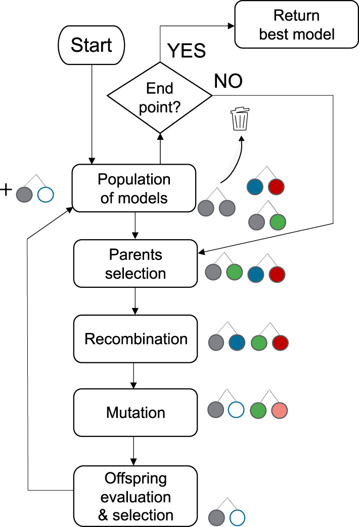
Flowchart of the genetic algorithm (adapted from Roland et al. 2021).
This procedure was repeated for at most 50 generations, and the best model from the final population was returned as result. Within the OSGA algorithm, each symbolic expression is represented as a parse tree (Figure 6), the length of which is given by the number of symbols (“nodes”) and whose depth is defined by the highest level of nesting (“longest branch”).
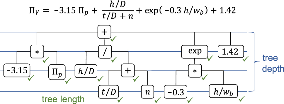
Example of a symbolic expression tree.
The settings for the symbolic regression are summarized in Table 2. As an extensive hyperparameter optimization would have been unaffordable, these settings were chosen based on common choices and educated guesses. To avoid unnecessarily complex models, the tree length and depth were both limited to a maximum value of 100, and the mathematical building blocks were restricted to the most common expressions in fluid dynamics theory. Furthermore, within the special functions, only sums and products of constants and variables were allowed as arguments. However, the limits for the tree length and depth are located generously high, favoring sophisticated models that capture the complex feature interactions in a three-dimensional curved channel flow. A mutation rate of 25 % was expected to yield quick improvements at the early stage of genetic programming, while preserving most high-quality models at the final stage. By allocating an extreme value of 100 for the maximum selection pressure, the evolutionary algorithm was exploited as long as possible, avoiding premature termination at the price of model quality.
Settings for the genetic algorithm.
| Max. tree length | 100 |
| Max. tree depth | 100 |
| Constants | All real numbers |
| Variables | All input features |
| Basic operations | +, *, /, 2 |
| Special functions without nesting | √, exp, ln, sin, cos |
| Population size | 1,000 |
| Crossover | Subtree swapping (90 % probability) |
| Mutation rate | 25 % |
| Max. selection pressure | 100 |
| Max. generations | 50 |
Since the algorithm contains random operations at several stages, even identical settings will yield models of different structure and quality. Thus, 36 runs were performed for each case to account for the statistical variations of the final models, using four desktop computers with 9 cores at 2.16 GHz clock frequency and 31.8 GB of RAM. The following properties of the regression models were evaluated:
the coefficient of determination R2 on all datasets,
the mean absolute error
the required training time,
model length and depth as measures of structural complexity.
The raw models were subsequently refined by an iterative pruning procedure in HeuristicLab to yield simpler expressions of similar prediction quality. During this process, redundant tree nodes were replaced with constants and the constants of the new model structure were optimized. Both steps were executed alternately for a maximum of 10 cycles until the model structure remained intact. In all cases, the coefficient of determination on the training set was virtually preserved, changing only beyond the sixth decimal digit.
Prior to the statistical evaluation, models with discontinuities or negative R2 in the extrapolation regime were discarded, as those predicted physically completely implausible trends. Such models typically showed poles from a division by zero or high-amplitude oscillations from trigonometric expressions. Moreover, samples were removed if their values were located further than three times the standard deviation away from the group mean (which again corresponded to exceptionally poor predictions). These two filtering steps led to more representative distributions of the model properties. The expected training time (ETT) for the first acceptable model was then estimated to
with (TT) i as training time for each individual model, Nruns as the number of runs (36 per stage), and Ndisc as the total number of discarded models.
The impact of domain knowledge on each model property was finally assessed by two criteria: (i) the median effects of each knowledge module compared to Case 1, and (ii) the statistical significance of each effect for a confidence level of 95 %. The corresponding p-values and confidence intervals were obtained from a two-sided Mood’s median test (Mood et al. 1974) within the statistical software package Minitab 22.1 (Minitab 2024). Comparisons between medians were preferred over means due to the highly variable model structures evolved by the genetic algorithm, which generally led to differently broad and up. In this case, the median is a more meaningful measure of an average model property.
4 Results and discussion
4.1 Prediction quality – interpolation
Figure 7a and Figure 8a compare the distributions of mean absolute errors and coefficients of determination, respectively, for all acceptable regression models on the interpolation dataset, as obtained for each case of data preprocessing. In general, all cases lead to excellent interpolation capability, with coefficients of determination greater than 0.9997 and mean absolute errors well below 0.01, which is in the order of ≤1 % of most dimensionless flow rates. Though the additional input features yield a statistically significant improvement in interpolation quality, as indicated by the confidence bars in Figure 7b and Figure 8b, the degree of improvement is rather small. The close match of the model predictions to the interpolation data can be attributed to the good coverage of the design space in the training dataset, which includes the boundary values of the chosen sub-range and a balanced distribution of design points in the interior with at least two intermediate levels for each parameter. Furthermore, only moderate nonlinearities exist in the interpolation dataset (Figure 3, Figure 4), which can be easily handled by the symbolic regression. Interpolation capability refers, in this study, to reliably predicting common settings for single-screw extrusion of polymers. As a result, if the regression models are intended exclusively for application in this common range, domain knowledge does not seem to bring a noteworthy benefit.
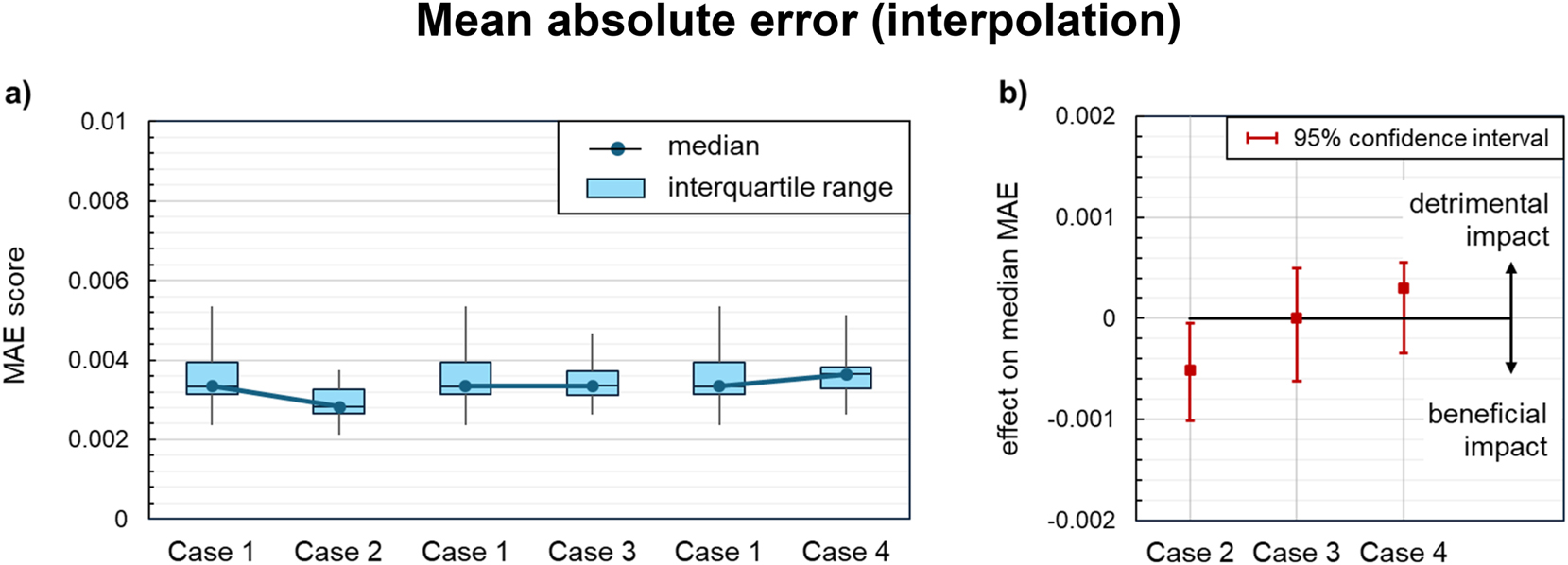
Impact of knowledge-driven data preprocessing on the mean absolute errors (MAE) of the symbolic regression models on the interpolation dataset: (a) MAE distribution across all acceptable models for each case of knowledge integration. (b) Effect on the median MAE compared to the baseline regression (case 1). Statistically significant effects are indicated by confidence intervals at a distance from the zero line.
4.2 Prediction quality – extrapolation
A different picture emerges when analyzing the prediction quality on the extrapolation dataset, as displayed in Figure 9 for the mean absolute error and Figure 10 for the coefficient of determination. Above all, the extrapolation accuracies are considerably lower compared to interpolation, which is not surprising, since the extreme nonlinearities in the extrapolation regime are not reflected in the training data (Figure 3, Figure 4). Furthermore, the model metrics fluctuate more intensely.
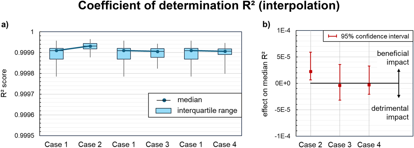
Impact of knowledge-driven data preprocessing on the coefficients of determination (R²) of the symbolic regression models on the interpolation dataset: (a) R² distribution across all acceptable models for each case of knowledge integration. (b) Effect on the median R2 compared to the baseline regression (case 1). Statistically significant effects are indicated by confidence intervals at a distance from the zero line.
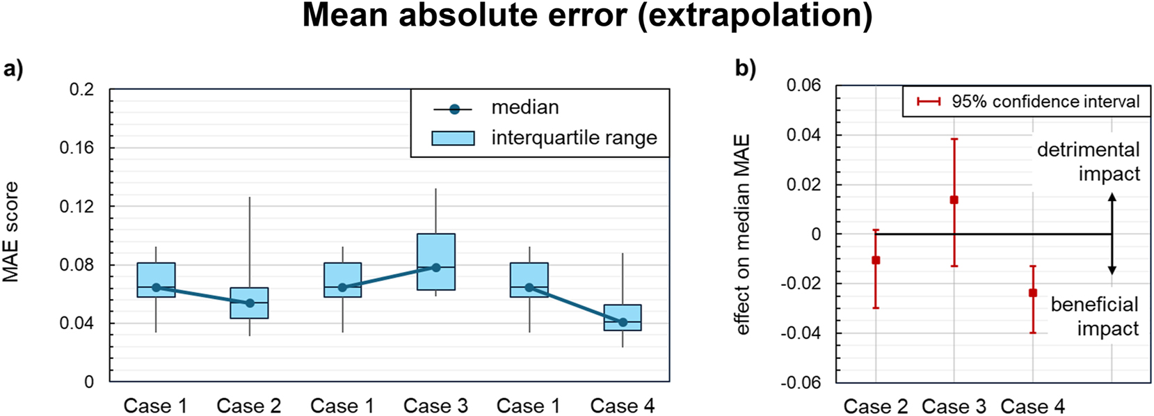
Impact of knowledge-driven data preprocessing on the mean absolute errors (MAE) of the symbolic regression models on the extrapolation dataset: (a) MAE distribution across all acceptable models for each case of knowledge integration. (b) Effect on the median MAE compared to the baseline regression (case 1). Statistically significant effects are indicated by confidence intervals at a distance from the zero line.
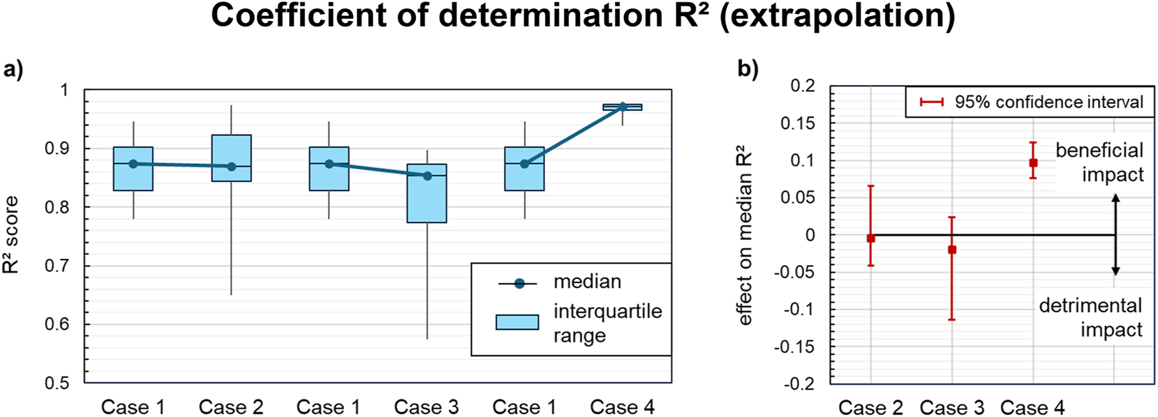
Impact of knowledge-driven data preprocessing on the coefficients of determination (R²) of the symbolic regression models on the extrapolation dataset: (a) R² distribution across all acceptable models for each case of knowledge integration. (b) Effect on the median R2 compared to the baseline regression (case 1). Statistically significant effects are indicated by confidence intervals at a distance from the zero line.
When comparing the quality metrics for each case of data preprocessing, larger median effects of each knowledge module are observed in the extrapolation regime. However, a statistically significant improvement was only achieved in Case 4, when the theoretical approximation equation was incorporated (Figure 9b, Figure 10b): Combining the approximation equation with symbolic regression models for the residuals reduced the median mean absolute error by 0.024 (−36 %) and raised the median coefficient of determination by roughly 0.1. As shown in Figure 9a and Figure 10a, both quality metrics also improved for the best models in Case 4, and the corresponding interquartile ranges became narrower, indicating higher robustness of the regression. None of these improvements could be observed for the other two cases. The superior performance of Case 4 is rooted in the fixed structure of the theoretical approximation, which encodes important interactions between the derived input features as opposed to Case 2 and reflects the asymptotic power-law behavior in contrast to Case 3. The theoretical approximation thus anticipates the main interrelations between the dimensionless extrusion variables and helps the regression procedure to generalize beyond the usual design space.
4.3 Prediction quality – localized accuracy
Besides a good overall prediction quality, the regression models should also achieve consistently high accuracy across different regions of the design space. To provide information on how the prediction accuracies vary locally, Figure 11 highlights the mean absolute errors, averaged over all acceptable models at each stage, for different bins of the power-law index n and the dimensionless down-channel pressure gradient Π p .
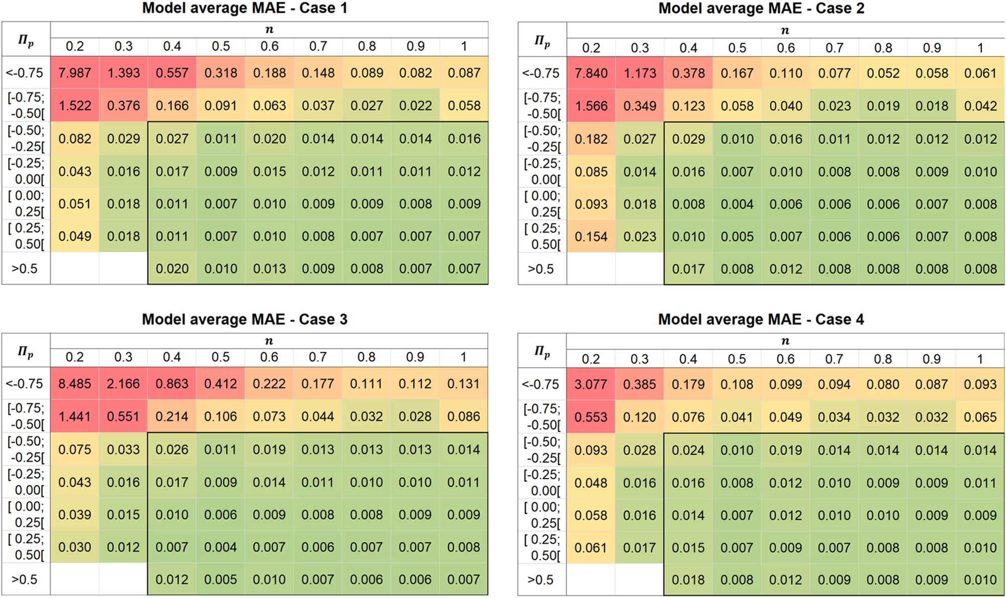
Heatmap of the model-averaged mean absolute error (MAE) for each level of n and sub-intervals for Π p , considering different cases of integrated domain knowledge. Poorer predictions are highlighted by higher numbers and a transition in background color from green to red. The thick black margin indicates the interpolation region for these two variables.
The interpolation region for these two variables is indicated by the thick black margin. Within this region, where the models extrapolate only along the h/D axis, all data preprocessing cases consistently lead to close approximations (1–5% of the target values). This can be explained by the minor influence of the channel depth ratio h/D on the dimensionless flow rate Π V in absolute terms. Hence, the training data represents the unseen design range for h/D quite well, and the benefits of domain knowledge are limited for these cases.
In the extrapolation regime, the prediction quality successively deteriorates with further distance from the interpolation boundary, providing large errors for bins with largest negative Π p and smallest n. These bins in the upper left corner contain data points with large Π V values, representing cases of dominant pressure flow, which strongly deviate from the training samples. The additional input features (Case 2) slightly improve the extrapolation capability for negative pressure gradients at the expense of accuracy for power law indices close to 0.2, while the opposite behavior is achieved by logarithmic scaling (Case 3). The high errors for the combined extrapolation remain almost unchanged in both cases. Including the theoretical approximation equation (Case 4), in contrast, drastically reduces the combined extrapolation error compared to Case 1 by a factor of two or three, and the errors within the remaining bins are also largely improved or maintained at low level. This effect is clearly visible by the lowest proportion of red color in the sub-figure. The models with the theoretical approximation equation thus achieve a considerably better-balanced performance on the entire design space and give substantially more robust predictions for the least familiar use cases.
The local error analysis further underlines the reasoning from the statistical evaluations why the theoretical approximation proves most beneficial for extrapolation: The key trends within the data, including the strong nonlinearities for the extreme cases in the upper left corner, are already represented in the approximation. As the regression algorithm no longer needs to infer these major trends but merely corrects the approximation for smaller influences on single-screw extrusion, there is an increased likelihood for models that capture the most important trends and thus provide a better overall explanation of the extrusion process.
4.4 Procedural efficiency and robustness
For a consistent usability of domain knowledge integration in symbolic regression analyses, the gain in accuracy should be achieved consistently within an acceptable processing time. As an indicator for the efficiency of the data-based modeling, Figure 12a plots the achieved R2 on the extrapolation dataset over the time for training the models. The ideal scenario is represented by the upper left corner of the figure – high yield in low time. Moreover, persistent high yields at low scattering indicate robustness.
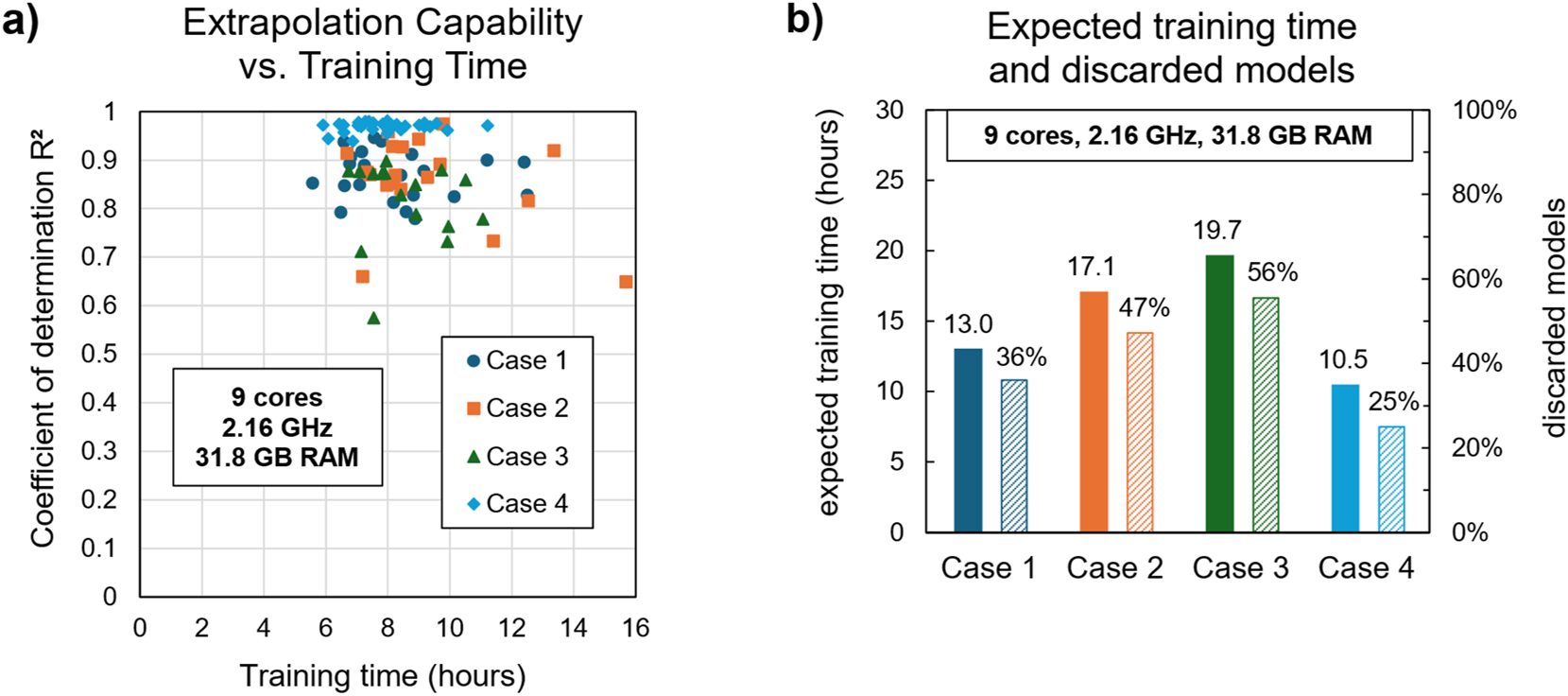
Computational efficiency of the symbolic regression for each case of domain knowledge integration: (a) Scatter plot of training times and coefficients of determination for each individual model and (b) bar chart showing the expected training times and fractions of discarded models for each case.
The scatter plot reveals that Case 2 occasionally yields models of higher quality but may also produce some low-quality instances or prolong the time for model creation. Consequently, the impact of the additional input features is highly sensitive with respect to the fluctuations in the regression algorithm. For Case 3, no clear improvement is evident either. Case 4, in contrast, consistently improves model quality at a similar distribution of training times: Almost all data points (light blue rhomboids) are clustered above those for Case 1 (dark blue circles). This again highlights the contribution of the theoretical approximation to an overall superior and more robust extrapolation capability.
The benefits of Case 4 become even more evident when factoring in the fraction of discarded models, as shown in Figure 12b: Both the number of bad-quality models and the expected training time are lowest if the theoretical approximation equation is included. Cases 2 and 3 even complicate the regression procedure compared to Case 1 by proposing more unrealistic solutions. Consequently, additional computational resources and longer expected training times are required for satisfactory model quality in those cases. With the theoretical approximation equation (Case 4), however, unrealistic solutions become less likely, making the regression analysis more robust and efficient.
4.5 Structural complexity
If critical decisions are to be inferred from model predictions, especially for industrial design or troubleshooting, too complex models may become impractical as they are hard to interpret. Each step of knowledge integration, in principle, adds a certain complexity to the total model. Concerning the practical utility of knowledge-based symbolic regression, the resulting complexity increase needs to be addressed alongside improvements in prediction quality.
To assess the added complexity of domain knowledge into the regression models, Figure 13 compares the expression tree lengths of the complete models for each case. It is striking that the median tree length increases by more than a factor of two when the theoretical approximation equation (Case 4) is applied to the data. This results from the high added complexity of the approximation equation itself, combined with the tendency of the OSGA to develop equally complex models for the residuals as for the complete target. Applying NSGA-II as an alternative algorithm would favor more simplistic models for the residuals; the sacrificed accuracy, however, turned out to be inacceptable in preliminary test runs. For the other cases, the tree lengths settled close to the upper limit of 100 for the regression, with similar medians and distributions. Hence, as expected, none of the integrated knowledge modules investigated guided the regression algorithm towards shorter models.
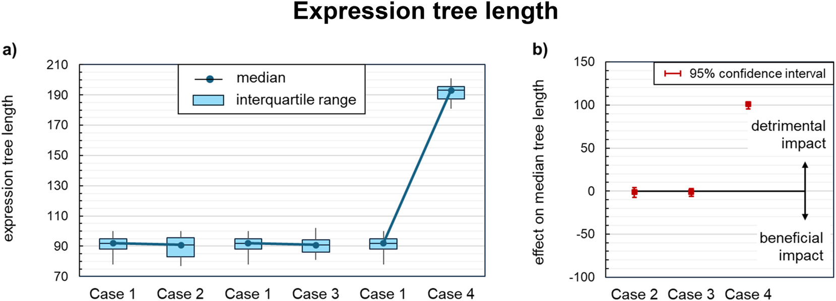
Impact of knowledge-driven data preprocessing on the expression tree lengths of the symbolic regression models: (a) Tree length distribution across all acceptable models for each case of knowledge integration. (b) Effect on the median tree length compared to the baseline regression (case 1). Statistically significant effects are indicated by confidence intervals at a distance from the zero line.
The tree depth, as shown in Figure 14a, is similar for all cases. Notably, no knowledge module attained a statistically significant effect (Figure 14b), which may appear counterintuitive at first glance. This is because Case 3 methodically introduced two supplementary levels of nesting through the exponential back-transformation, and Case 4 nearly doubled the total model size. However, as the complexity bias in Case 3 is only slight, it is obscured by the statistical variation of the algorithm. For Case 4, the theoretical approximation equation is generally less deep than the residual expression. Hence, the added length of the former does not inflate the total expression tree in depth.
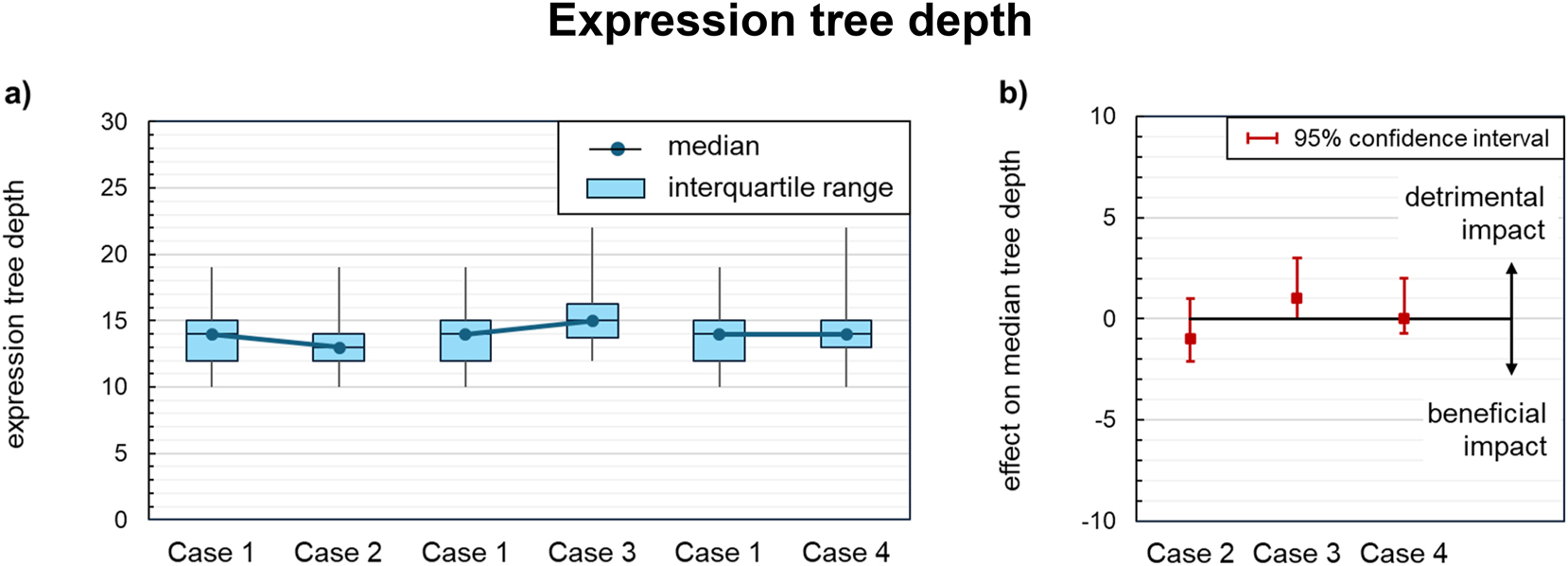
Impact of knowledge-driven data preprocessing on the expression tree depths of the symbolic regression models: (a) Tree depth distribution across all acceptable models for each case of knowledge integration. (b) Effect on the median tree depth compared to the baseline regression (case 1). Statistically significant effects are indicated by confidence intervals at a distance from the zero line.
In general, with more sophisticated data preprocessing, larger models will be obtained on average. If the respective preprocessing operations are sufficiently simple, however, the increase in complexity remains marginal compared to the inherent fluctuation of the algorithm. This is not the case for the theoretical approximation equation, where a double model size must be accepted for improved generalization. To increase the attractiveness of knowledge-based symbolic regression for polymer extrusion, lower tree length limits should be considered for the residual term in further studies. Although model depth and length omit certain aspects of model complexity, such as order and frequency of mathematical operations, these two measures already allow a conclusive assessment of the knowledge integration strategies investigated.
A visual impression of typical model structures is given in the appendix of this paper, showing the mathematical expressions of the best models for each case of integrated knowledge. The rating of the models was based on the coefficient of determination on the combined interpolation and extrapolation data, favoring shorter expressions in case of a tie. Each model consists of a main equation with 9–12 operators and 9–12 subfunctions that accept 35–55 coefficients in total, depending on the case. In any case, each input feature appears at least five times in the model equation, enters at least one nonlinear function, and feature interactions are considered up to third order. This largely explains the excellent interpolation capability of the regression models (Figure 8). At the same time, operators of constrained validity (e.g., divisions) are rare and well-conditioned, leading to reasonable extrapolation behavior (Figure 10). Admittedly, the model structures are generally highly sophisticated, and the parameter impacts are not clearly evident from the symbolic expressions alone. Due to the limitations explained in Section 2.1, however, the regression models in this study are not intended for standalone application; they rather serve as fast-computing sub-models in a superordinate extrusion calculation. In this setting, perfectly interpretable equations are of secondary importance, as engineering decisions will be based on numerical results from the global analysis. Although lower complexity limits are worth considering for further modeling efforts, they must be defined with caution to retain the predictive potential of the symbolic regression.
5 Conclusions
This study was intended to quantify the impact of domain knowledge integration on symbolic regression modeling of single-screw extrusion processes. The chosen database comprised more than 10,000 simulated design points for the dimensionless pumping characteristics of single-screw extruders, which was divided into three independent subsets: a (i) training and (ii) interpolation dataset covering common process settings, and (iii) an extrapolation subset including high-performance extrusion conditions. Aside from dimensional analysis, the training samples were preprocessed applying four cases of knowledge integration: (i) no further knowledge, (ii) additional input features derived from the independent flow parameters, (iii) logarithmic scaling of the dimensionless flow rate with one derived feature, and (iv) subtracting a theoretical approximation equation for unidirectional duct flow. The transformed dimensionless flow rate values were then approximated by symbolic regression using genetic programming with OSGA algorithm, yielding four sets of 36 analytical models for the dimensionless flow rate.
Statistical analysis of the models revealed that excellent interpolation capability was achievable in all cases, without a significant benefit of domain knowledge. Simultaneously, including the theoretical approximation equation led to significantly more robust and accurate extrapolations, especially in the region of strong nonlinearities. The theoretical approximation equation further reduced the expected training time for a physically reasonable model, rendering the regression analysis more efficient. These improvements, however, came at the price of increased model complexity. When deciding on a proper data-based modeling strategy for engineering tasks, such as screw design or process troubleshooting, the added complexity of the theoretical approximation must be weighed against the improved ability of the combined model to generalize.
To conclude, we recommend the following knowledge integration strategy for symbolic regression modeling in polymer extrusion: Initially, utilize the theory of similarity to identify the relevant physical features and harmonize the scales. In case of only modest nonlinearities in the dimensionless dataset that are below second-order or bounded within one decade, directly proceed with symbolic regression. If regions with more pronounced nonlinearities can be observed, approximate these nonlinear dependencies with a problem-related theoretical approximation, and determine symbolic regression models for the residuals.
A suggestion for future research would be to create residual models of reduced complexity, such that the total complexity remains similar, and to reassess the benefit of theoretical approximations under that circumstance. This measure could overcome the generalization-complexity trade-off introduced by the theoretical approximation equation. Another interesting research question concerns the impact of synthetic data from exact solutions and prior constraints on the function set. Both concepts represent additional pieces of domain knowledge that are likely to further enhance predictive power and efficiency of symbolic regression modeling in polymer extrusion.
Acknowledgments
Special thanks go to the team of the Institute of Polymer Product Engineering (IPPE) at the Johannes Kepler University of Linz for providing four powerful workstations to create the regression models. The authors further gratefully acknowledge Dr. Janos Birtha for reviewing the statistical evaluation.
-
Research ethics: Not applicable.
-
Informed consent: Not applicable.
-
Author contributions: Daniel Herzog: Conceptualization, Methodology, Software, Formal analysis, Data curation, Writing – Original Draft, Writing – Review & Editing, Visualization, Project Administration. Florian Lehner: Software, Investigation, Writing – Review & Editing, Visualization. Wolfgang Roland: Conceptualization, Methodology, Writing – Review & Editing, Funding Acquisition. Christian Marschik: Data Curation, Methodology, Investigation, Writing – Review & Editing. Gerald Berger-Weber: Resources, Writing – Review & Editing, Supervision, Funding Acquisition. All authors have accepted responsibility for the entire content of this manuscript and approved its submission.
-
Use of Large Language Models, AI and Machine Learning Tools: The free, web-based translator and style editor of DeepL (DeepL SE, Cologne, VAT-ID DE349242045) were consulted to translate German ideas into proper English and to rephrase drafted English text, respectively.
-
Conflict of interest: The authors state no conflict of interest.
-
Research funding: This work was supported in part by the Austrian Science Fund (FWF, grant DOI 10.55776/I4872). Christian Marschik further acknowledges financial support from the COMET Competence Center CHASE, which is managed by the Austrian Research Promotion Agency (FFG).
-
Data availability: The data that support the findings of this study are, if presented in figures and tables of this paper, openly available on Zenodo at http://doi.org/10.5281/zenodo.15045519 (Herzog et al., 2025a), http://doi.org/10.5281/zenodo.15043628, (Herzog et al., 2025b), http://doi.org/10.5281/zenodo.15045102 (Herzog et al. 2025c), http://doi.org/10.5281/zenodo.15044927 (Herzog et al., 2025d), http://doi.org/10.5281/zenodo.15044783 (Herzog et al., 2025e). Other data that support the findings of this study are available from the corresponding author, Daniel Herzog, upon reasonable request.
Appendix: Symbolic expressions
Best model for case 1
Best model for case 2
Best model for case 3
Best model for case 4
References
Albrecht, H., Roland, W., Fiebig, C., and Berger-Weber, G.R. (2022). Multi-dimensional regression models for predicting the wall thickness distribution of corrugated pipes. Polymers 14: 3455–3480, https://doi.org/10.3390/polym14173455.Search in Google Scholar PubMed PubMed Central
Ansys Inc. (2022). Ansys fluent user’s guide, release 2022R2. Ansys Inc, Canonsburg, PA.Search in Google Scholar
Campbell, G.A. and Spalding, M.A. (2013). Analyzing and troubleshooting single-screw extruders, 1st ed. Hanser Publishers, Munich/Cincinnati.10.3139/9783446432666.001Search in Google Scholar
Chitralekha, S.B. and Shah, S.L. (2010). Support Vector Regression for soft sensor design of nonlinear processes. In: 18th mediterranean conference on control and automation (MED´10). IEEE, Marrakech, Morocco, pp. 569–574.10.1109/MED.2010.5547730Search in Google Scholar
Hammer, A., Roland, W., Marschik, C., and Steinbichler, G. (2021). Predicting the co-extrusion flow of non-Newtonian fluids through rectangular ducts – a hybrid modeling approach. J. Non-Newt. Fluid Mech. 295: 104618, https://doi.org/10.1016/j.jnnfm.2021.104618.Search in Google Scholar
Herzog, D., Roland, W., Marschik, C., and Berger‐Weber, G.R. (2024). Generalized predictions of the pumping characteristics and viscous dissipation of single‐screw extruders including three‐dimensional curvature effects. Polym. Eng. Sci. 64: 5556–5587, https://doi.org/10.1002/pen.26934.Search in Google Scholar
Herzog, D. (2025a). Simulation data for the dimensionless pumping characteristics of single- screw extruders, v1. Zenodo. CERN, Geneva.Search in Google Scholar
Herzog, D. (2025b). Global prediction accuracies of knowledge-guided symbolic regression models for melt conveying in single-screw extruders, v1. Zenodo. CERN, Geneva.Search in Google Scholar
Herzog, D. (2025c). Localised prediction accuracies of knowledge-guided symbolic regression models for melt conveying in single-screw extruders, v1. Zenodo. CERN, Geneva.Search in Google Scholar
Herzog, D. (2025d). Training times and failure ratios of knowledge-guided symbolic regression models for melt conveying in single-screw extruders, v1. Zenodo. CERN, Geneva.Search in Google Scholar
Herzog, D. (2025e). Structural complexities of knowledge-guided symbolic regression models for melt conveying in single-screw extruders, v1. Zenodo. CERN, Geneva.Search in Google Scholar
Kowalski, R.J., Pietrysiak, E., and Ganjyal, G.M. (2021). Optimizing screw profiles for twin-screw food extrusion processing through genetic algorithms and neural networks. J. Food Eng. 303:110589: 1–6, https://doi.org/10.1016/j.jfoodeng.2021.110589.Search in Google Scholar
Kronberger, G., Burlacu, B., Kommenda, M., Winkler, S.M., and Affenzeller, M. (2025). Symbolic regression, 1st ed. CRC Press, Boca Raton, FL.10.1201/9781315166407-1Search in Google Scholar
Kronberger, G., de França, F.O., Burlacu, B., Haider, C., and Kommenda, M. (2022). Shape-constrained symbolic regression - improving extrapolation with prior knowledge. Evol. Comput. 30: 75–98, https://doi.org/10.1162/evco_a_00294.Search in Google Scholar PubMed
Kubalík, J., Derner, E., and Babuška, R. (2020). Symbolic regression driven by training data and prior knowledge. In: Genetic and evolutionary computation conference (GECCO’20). Association for Computing Machinery, Cancún, Mexico, pp. 958–966.10.1145/3377930.3390152Search in Google Scholar
La Cava, W.G., Lee, P.C., Ajmal, I., Ding, X., Solanki, P., Cohen, J.B., Moore, J.H., and Herman, D.S. (2023). A flexible symbolic regression method for constructing interpretable clinical prediction models. NPJ Digit. Med. 6: 107, https://doi.org/10.1038/s41746-023-00833-8.Search in Google Scholar PubMed PubMed Central
Li, Q., Zhang, C., Wei, Z., Jin, X., Shangguan, W., Yuan, H., Zhu, J., Li, L., Liu, P., Chen, X., et al.. (2024). Advancing symbolic regression for earth science with a focus on evapotranspiration modeling. NPJ Clim. Atmos. Sci. 7: 321, https://doi.org/10.1038/s41612-024-00861-5.Search in Google Scholar
Makke, N. and Chawla, S. (2024). Interpretable scientific discovery with symbolic regression: a review. Artif. Intell. Rev. 57: 2, https://doi.org/10.1007/s10462-023-10622-0.Search in Google Scholar
Marschik, C. and Roland, W. (2023a). Correction factors for the drag and pressure flows of power‐law fluids through rectangular ducts. Polym. Eng. Sci. 63: 2043–2058, https://doi.org/10.1002/pen.26344.Search in Google Scholar PubMed PubMed Central
Marschik, C. and Roland, W. (2023b). Predicting the pumping capability of single-screw extruders: a comparison of two- and three-dimensional modeling approaches. AIP Conf. Proc., 020002-1–020002-8 , https://doi.org/10.1063/5.0136774.Search in Google Scholar
Marschik, C., Roland, W., and Miethlinger, J. (2018). A network-theory-based comparative study of melt-conveying models in single-screw extrusion: A. isothermal flow. Polymers 10: 929–950, https://doi.org/10.3390/polym10080929.Search in Google Scholar PubMed PubMed Central
Marschik, C., Roland, W., and Osswald, T.A. (2022). Melt conveying in single-screw extruders: modeling and simulation. Polymers 14: 875–906, https://doi.org/10.3390/polym14050875.Search in Google Scholar PubMed PubMed Central
Marschik, C., Roland, W., and Kommenda, M. (2023). Extended melt‐conveying models for single‐screw extruders: integrating domain knowledge into symbolic regression. Polym. Eng. Sci. 63: 3639–3656, https://doi.org/10.1002/pen.26473.Search in Google Scholar
Matchev, K.T., Matcheva, K., and Roman, A. (2022). Analytical modeling of exoplanet transit spectroscopy with dimensional analysis and symbolic regression. ApJ 930: 33, https://doi.org/10.3847/1538-4357/ac610c.Search in Google Scholar
Minitab (2024). Minitab-unlock the value of your data with Minitab statistical software, Available at: https://www.minitab.com/content/dam/www/en/uploadedfiles/documents/brochures/Minitab-Brochure_EN.pdf.coredownload.inline.pdf (Accessed 14 March 2025).Search in Google Scholar
Molnar (2020). Interpretable machine learning: a guide for making black box models explainable, Available at: https://christophm.github.io/interpretable-ml-book/ (Accessed 20 May 2025).Search in Google Scholar
Mood, A.M., Graybill, F.A., and Boes, D.C. (1974). Introduction to the theory of statistics, 3rd ed. McGraw-Hill, New York.Search in Google Scholar
Pachner, S., Roland, W., Aigner, M., Marschik, C., Stritzinger, U., and Miethlinger, J. (2021). Using symbolic regression models to predict the pressure loss of non-Newtonian polymer-melt flows through melt-filtration systems with woven screens. Int. Polym. Process. 36: 435–450, https://doi.org/10.1515/ipp-2020-4019.Search in Google Scholar
Polychronopoulos, N.D., Moustris, K., Karakasidis, T., Sikora, J., Krasinskyi, V., Sarris, I.E., and Vlachopoulos, J. (2025). Machine learning for screw design in single‐screw extrusion. Polym. Eng. Sci. 65: 2607–2623, https://doi.org/10.1002/pen.27170.Search in Google Scholar
Potente, H., Bornemann, M., Heinrich, D., and Pape, J. (2005). Influence of power law and isothermal simplification on the accuracy in single screw extrusion. Int. Polym. Process. 20: 417–422, https://doi.org/10.1515/ipp-2005-0070.Search in Google Scholar
Roland, W., Kommenda, M., Marschik, C., and Miethlinger, J. (2019). Extended regression models for predicting the pumping capability and viscous dissipation of two-dimensional flows in single-screw extrusion. Polymers 11: 334–369, https://doi.org/10.3390/polym11020334.Search in Google Scholar PubMed PubMed Central
Roland, W., Marschik, C., Hammer, A., and Steinbichler, G. (2020). Modeling the non-isothermal conveying characteristics in single-screw extrusion by application of network analysis. SPE ANTEC Tech Papers.Search in Google Scholar
Roland, W., Marschik, C., Kommenda, M., Haghofer, A., Dorl, S., and Winkler, S. (2021). Predicting the non-linear conveying behavior in single-screw extrusion: a comparison of various data-based modeling approaches used with CFD simulations. Int. Polym. Process. 36: 529–544, https://doi.org/10.1515/ipp-2020-4094.Search in Google Scholar
Rauwendaal, C. (2014). Polymer extrusion, 5th ed. Hanser Publications, Munich/Cincinnati.10.3139/9781569905395.fmSearch in Google Scholar
Roland, W., Kommenda, M., and Berger-Weber, G. (2022). Application of symbolic regression in polymer processing. In: 24th international symposium on symbolic and numeric algorithms for scientific computing (SYNASC). IEEE, Hagenberg, Austria, pp. 311–318.10.1109/SYNASC57785.2022.00056Search in Google Scholar
Ronowicz, J., Thommes, M., Kleinebudde, P., and Krysiński, J. (2015). A data mining approach to optimize pellets manufacturing process based on a decision tree algorithm. Eur. J. Pharmaceut. Sci. 73: 44–48, https://doi.org/10.1016/j.ejps.2015.03.013.Search in Google Scholar PubMed
Rudin, C., Chen, C., Chen, Z., Huang, H., Semenova, L., and Zhong, C. (2022). Interpretable machine learning: fundamental principles and 10 grand challenges. Stat. Surv. 16: 1–85, https://doi.org/10.1214/21-ss133.Search in Google Scholar
Scheffold, L., Finkler, T., and Piechottka, U. (2021). Gray-Box system modeling using symbolic regression and nonlinear model predictive control of a semibatch polymerization. Comput. Chem. Eng. 146: 107204, https://doi.org/10.1016/j.compchemeng.2020.107204.Search in Google Scholar
Stritzinger, U., Roland, W., Berger‐Weber, G., and Steinbichler, G. (2023). Modeling melt conveying and power consumption of co‐rotating twin‐screw extruder kneading blocks: Part B. Prediction models. Polym. Eng. Sci. 63: 841–862, https://doi.org/10.1002/pen.26249.Search in Google Scholar
Tadmor, Z. and Klein, I. (1970). Engineering principles of plasticating extrusion. Van Nostrand Reinhold, New York, NY.Search in Google Scholar
Versino, D., Tonda, A., and Bronkhorst, C.A. (2017). Data driven modeling of plastic deformation. Comput. Methods Appl. Mech. Engrg. 318: 981–1004, https://doi.org/10.1016/j.cma.2017.02.016.Search in Google Scholar
Wagner, S., Kronberger, G., Beham, A., Kommenda, M., Scheibenpflug, A., Pfitzer, E., Vonolfen, S., Kofler, M., Winkler, S., Dorfer, V., et al.. (2014). Chapter 10 Architecture and design of the HeuristicLab optimization environment. In: Klempous, R., Nikodem, J., Jacak, W., and Chaczko, Z. (Eds.)., Advanced methods and applications of computational intelligence. Springer, Cham, Germany, pp. 197–261.10.1007/978-3-319-01436-4_10Search in Google Scholar
Zhou, S., Yang, B., Xiao, S., Yang, G., and Zhu, T. (2023). Crack growth rate model derived from domain knowledge-guided symbolic regression. Chin. J. Mech. Eng. 36: 40, https://doi.org/10.1186/s10033-023-00876-8.Search in Google Scholar
© 2025 the author(s), published by De Gruyter, Berlin/Boston
This work is licensed under the Creative Commons Attribution 4.0 International License.
Articles in the same Issue
- Frontmatter
- Review Articles
- A review on industrial optimization approach in polymer matrix composites manufacturing
- A review on the effect of fiber treatment and fillers on mechanical properties of kenaf fiber–reinforced composites
- Research Articles
- Synthesis of poly(methyl methacrylate) microspheres using poly(2-acrylamido-2-methylpropane sulfonic acid) as a suspending agent
- Medical grade polypropylene after artificial aging in regard to the VOC emissions
- Optimal performance of poly-hybrid nanocomposites promoted with carbon fibers and nano silicon carbide particles via compression associated with hot pressing: characterization study
- Spectroscopic analysis of silicone intraocular lenses by optical transmission measurements and FTIR
- Preparation and properties of biodegradable antibacterial polylactic acid/modified chitin antibacterial agent composites
- Impact of domain knowledge on developing pumping models for single-screw extruders using symbolic regression
- Calibrator modelling in the simulation of extrusion process
- Strength and thermophysical properties of polylactide-few-layer graphene composites