The area under the generalized receiver-operating characteristic curve
-
Pablo Martínez-Camblor

 ,
Sonia Pérez-Fernández
,
Sonia Pérez-Fernández

Abstract
The receiver operating-characteristic (ROC) curve is a well-known graphical tool routinely used for evaluating the discriminatory ability of continuous markers, referring to a binary characteristic. The area under the curve (AUC) has been proposed as a summarized accuracy index. Higher values of the marker are usually associated with higher probabilities of having the characteristic under study. However, there are other situations where both, higher and lower marker scores, are associated with a positive result. The generalized ROC (gROC) curve has been proposed as a proper extension of the ROC curve to fit these situations. Of course, the corresponding area under the gROC curve, gAUC, has also been introduced as a global measure of the classification capacity. In this paper, we study in deep the gAUC properties. The weak convergence of its empirical estimator is provided while deriving an explicit and useful expression for the asymptotic variance. We also obtain the expression for the asymptotic covariance of related gAUCs and propose a non-parametric procedure to compare them. The finite-samples behavior is studied through Monte Carlo simulations under different scenarios, presenting a real-world problem in order to illustrate its practical application. The R code functions implementing the procedures are provided as Supplementary Material.
Funding source: Ministerio de Ciencia e Innovación
Award Identifier / Grant number: MTM2015-63971-P
Funding source: Gobierno de Asturies
Award Identifier / Grant number: Severo Ochoa Grant BP16118
Funding source: Ministerio de Economia y Competitividad, Spain
Award Identifier / Grant number: MTM2014-55966-P
-
Author contribution: All the authors have actively participated in all aspects of this manuscript, all of them have read and approved the final version. All the authors have accepted responsibility for the entire content of this submitted manuscript and approved submission.
-
Research funding: This work is supported by the Grants MTM2015-63971-P and MTM2014-55966-P from the Spanish Ministerio of Economía y Competitividad, FC-15-GRUPIN14-101 and Severo Ochoa Grant BP16118 (this one for S. Pérez-Fernández) from the Asturies Government.
-
Conflict of interest statement: The authors have no conflicts of interest to report.
Technical issues
We are proving here the results enunciated along the manuscript. First, we provide the proof for the Proposition 1 (Section 2).
Proof of Proposition 1
Clearly, h(η) follows a uniform distribution between 0 and 1,
Analogously, the distribution function of h(ξ) is
And then,
□
Now, we will prove Theorems 1 (Section 3) and 2 (Section 4).
Proof of Theorem 1
We have that
In the last equality, we have considered that, for each p ∈ (0, 1), there exists α p ∈ [0, 1], such that [18]
Therefore, the assumption (F) guarantees that,
where
with X and Y two independent random variables distributed as ξ and η, respectively.
Hence, the Slutski’s lemma guarantees that the asymptotic distribution of
The central limit theorem’s assures the asymptotic normality of the above expression. Mean is clearly zero and, from the Proposition 1, the variance is
Proof of Theorem 2
Using similar notation that in the previous proof, we define
Arguing as in Theorem 1 proof’s we have to demonstrate the asymptotic normality of the random variable
We can apply again the TCL and get the normality of the above expression. Besides,
where F h (⋅, ⋅) is the distribution of h ( ξ ) = (h1(ξ1), h2(ξ2)). Analogously,
where
G
h
(⋅, ⋅) is the distribution of
h
(
η
) = (h1(η1), h2(η2)). Since
R code outlines
This is a brief example of the use of the implemented functions gROC and gAUC.test in order to estimate the gROC curve and to perform hypothesis testing for comparing gAUCs, respectively.
To import the database:

To compute the optimal gROC curve under restriction (C) for the markers WBC (white blood cells count) and LYM (lymphocytes percentage), respectively:

To compute the approx. optimal gROC curve under restriction (C) for WBC when the starting point 1 − Sp is 1/2:

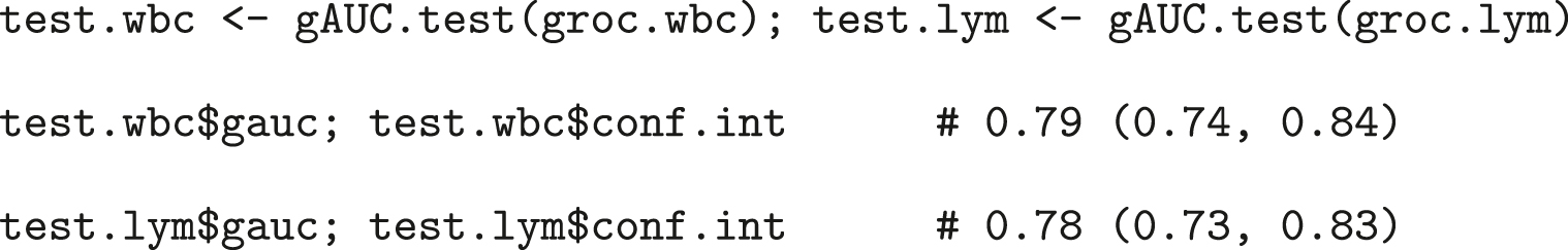
To compute a 95% confidence interval for gAUC of each marker:
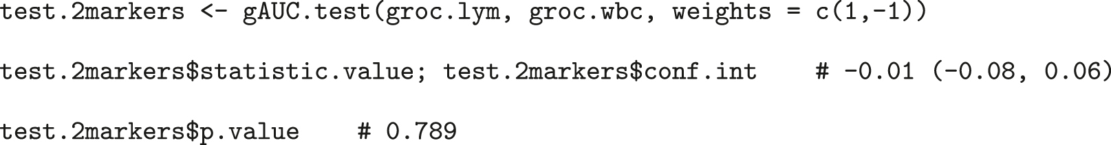
To compute a 95% confidence interval for the gAUC difference
References
1. Green, DM, Swets, JA. Signal detection theory and psychophysics. New York: Wiley; 1966.Search in Google Scholar
2. Hanley, JA, McNeil, BJ. The meaning and use of the area under a receiver operating characteristic (ROC) curve. Radiology 1982;143:29–36. https://doi.org/10.1148/radiology.143.1.7063747.Search in Google Scholar PubMed
3. Demidenko, E. The p-value you can’t buy. Am Statistician 2016;70:33–8. https://doi.org/10.1080/00031305.2015.1069760.Search in Google Scholar PubMed PubMed Central
4. Delong, ER, Delong, DM, Clarke-Pearson, DL. Comparing the areas under two or more correlated receiver operating characteristic curves: a nonparametric approach. Biometrics 1988;44:837–45. https://doi.org/10.2307/2531595.Search in Google Scholar
5. Braun, TM, Alonzo, TA. A modified sign test for comparing paired ROC curves. Biostatistics 2007;9:364–72. https://doi.org/10.1093/biostatistics/kxm036.Search in Google Scholar PubMed
6. Venkatraman, ES, Begg, CB. A distribution-free procedure for comparing receiver operating characteristic curves from a paired experiment. Biometrika 1996;83:835–48. https://doi.org/10.1093/biomet/83.4.835.Search in Google Scholar
7. Venkatraman, ES. A permutation test to compare receiver operating characteristic curves. Biometrics 2000;56:1134–8. https://doi.org/10.1111/j.0006-341x.2000.01134.x.Search in Google Scholar PubMed
8. Martínez Camblor, P, Carleos, C, Corral, N. Powerful nonparametric statistics to compare k independent ROC curves. J Appl Stat 2011;38:1317–32. https://doi.org/10.1080/02664763.2010.498504.Search in Google Scholar
9. Martínez-Camblor, P, Carleos, C, Corral, N. General nonparametric ROC curve comparison. J Korean Stat Soc 2013;42:71–81. https://doi.org/10.1016/j.jkss.2012.05.002.Search in Google Scholar
10. Hilden, J. The area under the ROC curve and its competitors. Med Decis Making 1991;11:95–101. https://doi.org/10.1177/0272989x9101100204.Search in Google Scholar
11. Yousef, WA. Assessing classifiers in terms of the partial area under the ROC curve. Comput Stat Data Anal 2013;64:51–70. https://doi.org/10.1016/j.csda.2013.02.032.Search in Google Scholar
12. Pardo, MC, Franco-Pereira, AM. Non parametric ROC summary statistics. REVSTAT 2017;15:583–600 .Search in Google Scholar
13. McIntosh, MW, Pepe, MS. Combining several screening tests: optimality of the risk score. Biometrics 2002;58:657–64. https://doi.org/10.1111/j.0006-341x.2002.00657.x.Search in Google Scholar PubMed
14. Metz, CE, Pan, X. ‘Proper’ binormal ROC curves: theory and maximum-likelihood estimation. J Math Psychol 1999;43:1–33. https://doi.org/10.1006/jmps.1998.1218.Search in Google Scholar PubMed
15. Qin, J, Zhang, B. Best combination of multiple diagnostic tests for screening purposes. Stat Med 2010;29:2905–19. https://doi.org/10.1002/sim.4068.Search in Google Scholar PubMed
16. Chen, B, Li, P, Qin, J, Yu, T. Using a monotonic density ratio model to find the asymptotically optimal combination of multiple diagnostic tests. J Am Stat Assoc 2016;111:861–74. https://doi.org/10.1080/01621459.2015.1066681.Search in Google Scholar
17. Martínez-Camblor, P, Pérez-Fernández, S, Díaz-Coto, S. Optimal classification scores based on multivariate marker transformations. AStA Adv Stat Anal 2021;1–16. https://doi.org/10.1007/s10182-020-00388-z. In press.Search in Google Scholar
18. Martínez-Camblor, P, Corral, N, Rey, C, Pascual, J, Cernuda-Morollón, E. Receiver operating characteristic curve generalization for non-monotone relationships. Stat Methods Med Res 2017;26:113–23. https://doi.org/10.1177/0962280214541095.Search in Google Scholar PubMed
19. Martínez-Camblor, P, Pérez-Fernández, S, Díaz-Coto, S. Improving the biomarker diagnostic capacity via functional transformations. J Appl Stat 2019;46:1550–66. https://doi.org/10.1080/02664763.2018.1554628.Search in Google Scholar
20. Martínez-Camblor, P, Pardo-Fernández, JC. Parametric estimates for the receiver operating characteristic curve generalization for non-monotone relationships. Stat Methods Med Res 2019;28:2032–48. https://doi.org/10.1177/0962280217747009.Search in Google Scholar PubMed
21. Zhou, XH, McClish, DK, Obuchowski, NA. Statistical methods in diagnostic medicine. In: Series in probability and statistics. New York, NY: Wiley Blackwell; 2002.10.1002/9780470317082Search in Google Scholar
22. Pepe, MS. The statistical evaluation of medical tests for classification and prediction. Oxford statistical science series. Oxford: Oxford University Press; 2003.10.1093/oso/9780198509844.001.0001Search in Google Scholar
23. Krzanowski, W, Hand, D. ROC curves for continuous data. New York: Chapman and Hall/CRC; 2009.10.1201/9781439800225Search in Google Scholar
24. Pérez-Fernández, S, Martínez-Camblor, P, Filzmoser, P, Corral, N. Visualizing the decision rules behind the ROC curves: understanding the classification process. AStA Adv Stat Anal 2021;105:135–61. https://doi.org/10.1007/s10182-020-00385-2.Search in Google Scholar
25. Martínez-Camblor, P, Pardo-Fernández, JC. The Youden index in the generalized receiver operating characteristic curve context. Int J Biostat 2019;15:1–20. https://doi.org/10.1515/ijb-2018-0060.Search in Google Scholar PubMed
26. Spanos, A, Harrell, FE, Durack, DT. Differential diagnosis of acute meningitis: an analysis of the predictive value of initial observations. J Am Med Assoc 1989;262:2700–7. https://doi.org/10.1001/jama.262.19.2700.Search in Google Scholar
27. Martínez-Camblor, P. Area under the ROC curve comparison in the presence of missing data. J Korean Surg Soc 2013;42:431–42. https://doi.org/10.1016/j.jkss.2013.01.004.Search in Google Scholar
28. Mossman, D. Three-way ROCs. Med Decis Making 1999;19:78–89. https://doi.org/10.1177/0272989x9901900110.Search in Google Scholar
29. Nakas, C, Yiannoutsos, T. Ordered multiple-class roc analysis with continuous measurements. Stat Med 2004;23:3437–49. https://doi.org/10.1002/sim.1917.Search in Google Scholar PubMed
30. van der Vaart AW . Asymptotic statistics. In: Series in statistical and probabilistic mathematics. Cambridge: Cambridge University Press; 1998.10.1017/CBO9780511802256Search in Google Scholar
Supplementary Material
The online version of this article offers supplementary material (https://doi.org/10.1515/ijb-2020-0091).
© 2021 Walter de Gruyter GmbH, Berlin/Boston
Articles in the same Issue
- Frontmatter
- Research Articles
- Integrating additional knowledge into the estimation of graphical models
- Asymptotic properties of the two one-sided t-tests – new insights and the Schuirmann-constant
- Bayesian optimization design for finding a maximum tolerated dose combination in phase I clinical trials
- A Bayesian mixture model for changepoint estimation using ordinal predictors
- Power prior for borrowing the real-world data in bioequivalence test with a parallel design
- Bayesian approaches to variable selection: a comparative study from practical perspectives
- Bayesian adaptive design of early-phase clinical trials for precision medicine based on cancer biomarkers
- More than one way: exploring the capabilities of different estimation approaches to joint models for longitudinal and time-to-event outcomes
- Designing efficient randomized trials: power and sample size calculation when using semiparametric efficient estimators
- Power formulas for mixed effects models with random slope and intercept comparing rate of change across groups
- The effect of data aggregation on dispersion estimates in count data models
- A zero-inflated non-negative matrix factorization for the deconvolution of mixed signals of biological data
- Multiple scaled symmetric distributions in allometric studies
- Estimation of semi-Markov multi-state models: a comparison of the sojourn times and transition intensities approaches
- Regularized bidimensional estimation of the hazard rate
- The effect of random-effects misspecification on classification accuracy
- The area under the generalized receiver-operating characteristic curve