More than one way: exploring the capabilities of different estimation approaches to joint models for longitudinal and time-to-event outcomes
-
Anja Rappl
 ,
Andreas Mayr
,
Andreas Mayr

Abstract
The development of physical functioning after a caesura in an aged population is still widely unexplored. Analysis of this topic would need to model the longitudinal trajectories of physical functioning and simultaneously take terminal events (deaths) into account. Separate analysis of both results in biased estimates, since it neglects the inherent connection between the two outcomes. Thus, this type of data generating process is best modelled jointly. To facilitate this several software applications were made available. They differ in model formulation, estimation technique (likelihood-based, Bayesian inference, statistical boosting) and a comparison of the different approaches is necessary to identify their capabilities and limitations. Therefore, we compared the performance of the packages JM, joineRML, JMbayes and JMboost of the R software environment with respect to estimation accuracy, variable selection properties and prediction precision. With these findings we then illustrate the topic of physical functioning after a caesura with data from the German ageing survey (DEAS). The results suggest that in smaller data sets and theory driven modelling likelihood-based methods (expectation maximation, JM, joineRML) or Bayesian inference (JMbayes) are preferable, whereas statistical boosting (JMboost) is a better choice with high-dimensional data and data exploration settings.
- 3
Note: Anja Rappl performed the present work in partial fulfilment of the requirements for obtaining the degree ‘Dr. rer. biol. hum.’ at Friedrich-Alexander-Universität Erlangen-Nürnberg.
-
Author contribution: All the authors have accepted responsibility for the entire content of this submitted manuscript and approved submission.
-
Research funding: The work on this article was supported by the DFG (Projekt WA 4249/2-1) and the Volkswagen Foundation.
-
Conflict of interest statement: The authors declare no conflicts of interest regarding this article.
Calculation of MSE
Average MSE-values by model and software.
| Model | Parameter | JM | joineRML | JMbayes | JMboost |
|---|---|---|---|---|---|
| AM1 | β l0 | 0.026 | 0.028 | 0.029 | 0.039 |
| β ls1 | 0.026 | 0.025 | 0.024 | 0.031 | |
| β ls2 | 0.019 | 0.018 | 0.020 | 0.028 | |
| β ls3 | 0.026 | 0.028 | 0.026 | 0.037 | |
| β ls4 | 0.017 | 0.018 | 0.018 | 0.024 | |
| β ls5 | 0.027 | 0.026 | 0.025 | 0.029 | |
| β ls6 | 0.025 | 0.028 | 0.030 | 0.037 | |
| β ls7 | 0.027 | 0.028 | 0.028 | 0.035 | |
| β ls8 | 0.028 | 0.028 | 0.026 | 0.037 | |
| β ls9 | 0.019 | 0.019 | 0.020 | 0.023 | |
| β ls10 | 0.021 | 0.022 | 0.023 | 0.029 | |
| β t | 0.016 | 0.016 | 0.017 | 0.130 | |
| β s | 0.038 | 0.042 | 0.042 | 0.038 | |
| α | 0.007 | 0.031 | 0.007 | 0.011 | |
| σ 2 | 0.040 | 0.002 | 0.035 | 1.019 | |
| B 00 | 0.169 | 0.164 | 0.141 | ||
| B 01/10 | 0.028 | 0.028 | 0.084 | ||
| B 11 | 0.029 | 0.028 | 337.920 | ||
| AM2 | β l0 | 0.026 | 0.026 | 0.056 | 0.044 |
| β l1 | 0.002 | 0.002 | 0.002 | 0.135 | |
| β l2 | 0.002 | 0.002 | 0.002 | 0.132 | |
| β l3 | 0.002 | 0.002 | 0.002 | 0.131 | |
| β l4 | 0.002 | 0.002 | 0.002 | 0.082 | |
| β l5 | 0.001 | 0.001 | 0.001 | 0.137 | |
| β l6 | 0.001 | 0.001 | 0.001 | 0.121 | |
| β t | 0.021 | 0.021 | 0.019 | 0 | |
| β s | 0.048 | 0.050 | 0.052 | 0.033 | |
| α | 0.013 | 0.029 | 0.014 | Inf | |
| σ 2 | 0.039 | 0.002 | 0.036 | 1.444 | |
| B 00 | 0.115 | 0.113 | 0.097 | ||
| B 01/10 | 0.042 | 0.041 | 0.099 | ||
| B 11 | 0.034 | 0.033 | 126.073 | ||
| AM3 | β l0 | 0.028 | 0.028 | 0.032 | 0.040 |
| β l1 | 0.002 | 0.002 | 0.002 | 0.150 | |
| β l2 | 0.002 | 0.002 | 0.002 | 0.144 | |
| β l3 | 0.002 | 0.002 | 0.002 | 0.141 | |
| β l4 | 0.002 | 0.002 | 0.002 | 0.082 | |
| β l5 | 0.001 | 0.001 | 0.001 | 0.149 | |
| β ls1 | 0.022 | 0.022 | 0.238 | 0.031 | |
| β ls2 | 0.024 | 0.023 | 0.037 | 0.029 | |
| β ls3 | 0.023 | 0.023 | 0.296 | 0.030 | |
| β ls4 | 0.023 | 0.022 | 0.020 | 0.024 | |
| β ls5 | 0.027 | 0.026 | 0.051 | 0.030 | |
| β t | 0.021 | 0.022 | 0.032 | 0.160 | |
| β s | 0.044 | 0.044 | 0.047 | 0.040 | |
| α | 0.008 | 0.026 | 0.008 | 0.022 | |
| σ 2 | 0.039 | 0.002 | 0.037 | 1.298 | |
| B 00 | 0.125 | 0.128 | 0.093 | ||
| B 01/10 | 0.041 | 0.040 | 0.113 | ||
| B 11 | 0.035 | 0.034 | 620.771 |
See Table 5.
Median of false-positive and -negative rates of packages by model and dimensionality.
| Model | Software | No. of available simulations | No. of failures | Median false-positive rate [min; max] | Median false-negative rate [min; max] |
|---|---|---|---|---|---|
| V1M1 | JM | 96 | 4 | 0.846 [0.538; 0.923] | 0.000 [0.000; 1.000] |
| joineRML | 100 | 0 | 0.923 [0.692; 0.923] | 0.000 [0.000; 0.500] | |
| JMbayes | 88 | 12 | 0.923 [0.692; 0.923] | 0.000 [0.000; 0.500] | |
| JMboost | 100 | 0 | 0.538 [0.231; 0.769] | 0.188 [0.062; 0.375] | |
| V1M2 | JM | 98 | 2 | 0.923 [0.538; 0.923] | 0.000 [0.000; 1.000] |
| joineRML | 99 | 1 | 0.923 [0.769; 0.923] | 0.000 [0.000; 0.500] | |
| JMbayes | 83 | 17 | 0.923 [0.692; 0.923] | 0.000 [0.000; 1.000] | |
| JMboost | 100 | 0 | 0.385 [0.077; 0.538] | 0.375 [0.167; 0.583] | |
| V1M3 | JM | 95 | 5 | 0.923 [0.615; 0.923] | 0.000 [0.000; 1.000] |
| joineRML | 100 | 0 | 0.923 [0.615; 0.923] | 0.000 [0.000; 0.500] | |
| JMbayes | 77 | 23 | 0.923 [0.769; 0.923] | 0.000 [0.000; 1.000] | |
| JMboost | 97 | 3 | 0.462 [0.154; 0.692] | 0.312 [0.125; 0.562] | |
| V2M1 | JM | 2 | 98 | 0.764 [0.750; 0.777] | 0.250 [0.000; 0.500] |
| joineRML | 2 | 98 | 0.659 [0.635; 0.682] | 0.500 [0.500; 0.500] | |
| JMbayes | 0 | 100 | |||
| JMboost | 100 | 0 | 0.128 [0.061; 0.223] | 0.438 [0.188; 0.625] | |
| V2M2 | JM | 10 | 90 | 0.818 [0.730; 0.912] | 0.000 [0.000; 0.500] |
| joineRML | 1 | 99 | 0.676 [0.676; 0.676] | 0.500 [0.500; 0.500] | |
| JMbayes | 0 | 100 | |||
| JMboost | 100 | 0 | 0.068 [0.041; 0.270] | 0.500 [0.250; 0.667] | |
| V2M3 | JM | 12 | 88 | 0.780 [0.676; 0.865] | 0.000 [0.000; 1.000] |
| joineRML | 1 | 99 | 0.649 [0.649; 0.649] | 0.500 [0.500; 0.500] | |
| JMbayes | 0 | 100 | |||
| JMboost | 100 | 0 | 0.088 [0.027; 0.331] | 0.438 [0.250; 0.688] | |
| V3M1 | JM | 0 | 100 | ||
| joineRML | 0 | 100 | |||
| JMbayes | 0 | 100 | |||
| JMboost | 100 | 0 | 0.028 [0.013; 0.056] | 0.562 [0.250; 0.875] | |
| V3M2 | JM | 0 | 100 | ||
| joineRML | 0 | 100 | |||
| JMbayes | 0 | 100 | |||
| JMboost | 100 | 0 | 0.020 [0.011; 0.057] | 0.500 [0.333; 0.667] | |
| V3M3 | JM | 0 | 100 | ||
| joineRML | 0 | 100 | |||
| JMbayes | 0 | 100 | |||
| JMboost | 100 | 0 | 0.019 [0.007; 0.123] | 0.562 [0.375; 0.750] |
Calculation of MSPE for longitudinal outcomes
Calculation of MSPE for survival outcomes
MSPE-values for marginal prediction of longitudinal outcome by model, dimensionality and package.
| Dimension | Model | JM | joineRML | JMbayes | JMboost |
|---|---|---|---|---|---|
| PA | M1 | 2.76 [2.47; 3.12] | 2.77 [2.46; 3.32] | 2.77 [2.47; 3.23] | 2.82 [2.49; 3.44] |
| PA | M2 | 2.53 [2.30; 2.83] | 2.53 [2.30; 2.83] | 2.54 [2.35; 3.02] | 3.22 [2.83; 3.83] |
| PA | M3 | 2.63 [2.39; 3.19] | 2.63 [2.40; 3.18] | 3.21 [2.44; 4.04] | 3.30 [2.96; 4.04] |
| PV1 | M1 | 2.94 [2.56; 3.43] | 2.95 [2.56; 3.46] | 2.82 [2.50; 3.37] | 2.99 [2.51; 3.59] |
| PV1 | M2 | 2.63 [2.34; 3.07] | 2.64 [2.35; 3.08] | 2.57 [2.36; 3.18] | 3.25 [2.87; 3.83] |
| PV1 | M3 | 2.76 [2.47; 3.21] | 2.77 [2.47; 3.22] | 3.29 [2.66; 3.91] | 3.44 [2.99; 4.14] |
| PV2 | M1 | 6.28 [5.67; 6.89] | 6.65 [6.03; 7.27] | 3.54 [2.79; 4.74] | |
| PV2 | M2 | 4.70 [4.00; 6.24] | 4.64 [4.64; 4.64] | 3.21 [2.86; 3.83] | |
| PV2 | M3 | 5.40 [4.40; 6.24] | 5.89 [5.89; 5.89] | 3.71 [3.18; 5.83] | |
| PV3 | M1 | 4.17 [3.29; 7.35] | |||
| PV3 | M2 | 3.23 [2.87; 3.80] | |||
| PV3 | M3 | 4.14 [3.32; 6.23] |
MSPE-values for subject-specific prediction of the survival probability by model, dimensionality and package.
| Dimension | Model | JM | joineRML | JMbayes | JMboost |
|---|---|---|---|---|---|
| PA | M1 | 0.12 [0.08; 0.19] | 0.24 [0.12; 0.44] | 0.11 [0.08; 0.14] | 0.14 [0.11; 0.16] |
| PA | M2 | 0.13 [0.09; 0.20] | 0.23 [0.13; 0.42] | 0.11 [0.09; 0.14] | |
| PA | M3 | 0.13 [0.10; 0.21] | 0.24 [0.12; 0.43] | 0.11 [0.09; 0.14] | 0.14 [0.11; 0.17] |
| PV1 | M1 | 0.13 [0.08; 0.20] | 0.24 [0.12; 0.44] | 0.11 [0.09; 0.14] | 0.14 [0.11; 0.17] |
| PV1 | M2 | 0.13 [0.09; 0.20] | 0.23 [0.13; 0.42] | 0.11 [0.09; 0.14] | 0.14 [0.11; 0.17] |
| PV1 | M3 | 0.13 [0.10; 0.22] | 0.24 [0.12; 0.43] | 0.11 [0.09; 0.14] | 0.14 [0.11; 0.17] |
| PV2 | M1 | 0.13 [0.13; 0.13] | 0.31 [0.30; 0.33] | 0.14 [0.11; 0.17] | |
| PV2 | M2 | 0.14 [0.12; 0.15] | 0.14 [0.14; 0.14] | 0.14 [0.11; 0.17] | |
| PV2 | M3 | 0.12 [0.11; 0.16] | 0.16 [0.16; 0.16] | 0.14 [0.12; 0.17] | |
| PV3 | M1 | 0.14 [0.11; 0.17] | |||
| PV3 | M2 | 0.14 [0.11; 0.17] | |||
| PV3 | M3 | 0.14 [0.11; 101293.98] |
The update mechanism of statistical boosting algorithms yield characteristic coefficient paths across their set iteration times. They reflect that per iteration only one coefficient per gradient is updated by a small proportion, that coefficients are selected at different times throughout the algorithm and that earlier selected coefficients tend to be larger once the algorithm stops. An example of a standard image of coefficient paths is given in Figure 9.
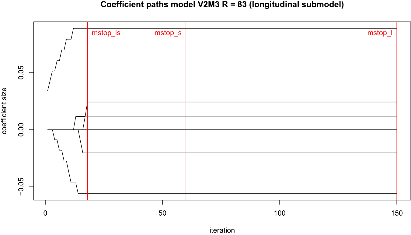
Ideal behaviour of coefficient paths in statistical boosting.
In comparison Figure 10 shows the coefficient paths of the data example of “healthy ageing”. The paths oscillate heavily, which is a sign of instability. This becomes particularly problematic with the effect of obstime, since it alternates between positive and negative values. The values for mstop_l, mstop_ls and mstop_s indicate the optimal iteration number for the predicted likelihood to be at its minimum (cross-validation). A potential remedy for this behaviour is for the algorithm to be forced to run longer at the compromise of less optimal prediction. In this case, however, the oscillation will not stop even when the iteration numbers are increased. Thus, boosting will not yield entirely satisfying results for this data problem.
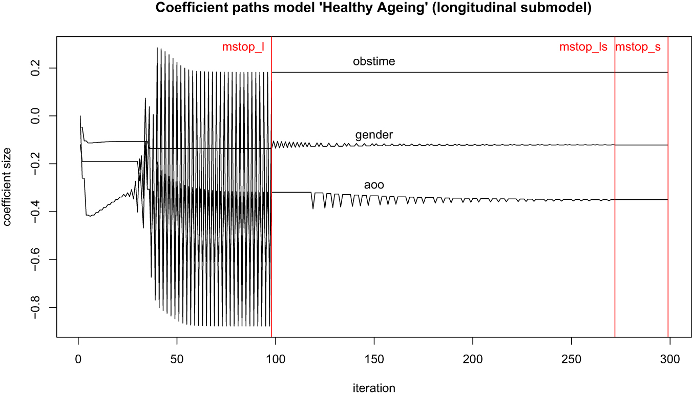
Suboptimal trajectory of coefficient paths of the data model “healthy ageing” when boosted.
References
1. WHO. World report on ageing and health. Geneva: WHO; 2015.Search in Google Scholar
2. Henderson, R, Diggle, P, Dobson, A. Joint modelling of longitudinal measurements and event time data. Biostatistics 2000;1:465–80. https://doi.org/10.1093/biostatistics/1.4.465.Search in Google Scholar
3. Wulfsohn, MS, Tsiatis, AA. A joint model for survival and longitudinal data measured with error. Biometrics 1997;53:330–39. https://doi.org/10.2307/2533118.Search in Google Scholar
4. Rizopoulos, D. Joint models for longitudinal and time-to-event data: With applications in R. In: Chapman & Hall/CRC biostatistics series, vol 6. Boca Raton: CRC Press; 2012.10.1201/b12208Search in Google Scholar
5. Song, X, Davidian, M, Tsiatis, AA. A semiparametric likelihood approach to joint modeling of longitudinal and time-to-event data. Biometrics 2002;58:742–53. https://doi.org/10.1111/j.0006-341x.2002.00742.x.Search in Google Scholar
6. Hsieh, F, Tseng, Y-K, Wang, J-L. Joint modeling of survival and longitudinal data: likelihood approach revisited. Biometrics 2006;62:1037–43. https://doi.org/10.1111/j.1541-0420.2006.00570.x.Search in Google Scholar
7. Tseng, Y-K, Hsieh, F, Wang, J-L. Joint modelling of accelerated failure time and longitudinal data. Biometrika 2005;92:587–603. https://doi.org/10.1093/biomet/92.3.587.Search in Google Scholar
8. Lin, H, McCulloch, CE, Mayne, ST. Maximum likelihood estimation in the joint analysis of time-to-event and multiple longitudinal variables. Stat Med 2002;21:2369–82. https://doi.org/10.1002/sim.1179.Search in Google Scholar
9. Asar, O, Ritchie, J, Kalra, PA, Diggle, PJ. Joint modelling of repeated measurement and time-to-event data: an introductory tutorial. Int J Epidemiol 2015;44:334–44. https://doi.org/10.1093/ije/dyu262.Search in Google Scholar
10. Tsiatis, AA, Davidian, M. Joint modeling of longitudinal and time-to-event data: an overview. Stat Sin 2004;14:809–34.Search in Google Scholar
11. Faucett, CL, Thomas, DC. Simultaneously modelling censored survival data and repeatedly measured covariates: a Gibbs sampling approach. Stat Med 1996;15:1663–85. https://doi.org/10.1002/(sici)1097-0258(19960815)15:15<1663::aid-sim294>3.0.co;2-1.10.1002/(SICI)1097-0258(19960815)15:15<1663::AID-SIM294>3.0.CO;2-1Search in Google Scholar
12. Waldmann, E, Taylor-Robinson, D, Klein, N, Kneib, T, Pressler, T, Schmid, M, et al.. Boosting joint models for longitudinal and time-to-event data. Biom J 2017;59:1104–21. https://doi.org/10.1002/bimj.201600158.Search in Google Scholar
13. R Core Team. R: A language and environment for statistical computing. Vienna, Austria: R Foundation for Statistical Computing; 2019. Available from: https://www.r-project.org.Search in Google Scholar
14. SAS Institute Inc. The SAS system, version 9.4. Cary: SAS Institute Inc.; 2013. Available from: https://www.sas.com/.Search in Google Scholar
15. StataCorp. Stata Statistical Software: release 16. College Station, TX: StataCorp LLC; 2019. Available from: https://www.stata.com/.Search in Google Scholar
16. Lunn, DJ, Thomas, A, Best, N, Spiegelhalter, D. WinBUGS – a bayesian modelling framework: concepts, structure, and extensibility. Stat Comput 2000;10:325–37. https://doi.org/10.1023/a:1008929526011.10.1023/A:1008929526011Search in Google Scholar
17. Rizopoulos, D. JM: an R package for the joint modelling of longitudinal and time-to-event data. J Stat Software 2010;35. https://doi.org/10.18637/jss.v035.i09.10.18637/jss.v035.i09Search in Google Scholar
18. Philipson, P, Sousa, I, Diggle, PJ, Williamson, P, Kolamunnage-Dona, R, Henderson, R, et al.. joineR: joint modelling of repeated measurements and time-to-event data. CRAN; 2017. Available from: https://github.com/graemeleehickey/joineR/.Search in Google Scholar
19. Hickey, GL, Philipson, P, Jorgensen, A, Kolamunnage-Dona, R. joineRML: a joint model and software package for time-to-event and multivariate longitudinal outcomes. BMC Med Res Methodol 2018;18:50. https://doi.org/10.1186/s12874-018-0502-1.Search in Google Scholar PubMed PubMed Central
20. Guo, X, Carlin, BP. Separate and joint modeling of longitudinal and event time data using standard computer packages. Am Statistician 2004;58:16–24. https://doi.org/10.1198/0003130042854.Search in Google Scholar
21. Crowther, MJ, Abrams, KR, Lambert, PC. Joint modeling of longitudinal and survival data. STATA J 2013;13:165–84. https://doi.org/10.1177/1536867x1301300112.Search in Google Scholar
22. Rizopoulos, D. The R package JMbayes for fitting joint models for longitudinal and time-to-event data using MCMC. J Stat Software 2016;72. https://doi.org/10.18637/jss.v072.i07.Search in Google Scholar
23. Yuen, HP, Mackinnon, A. Performance of joint modelling of time-to-event data with time-dependent predictors: an assessment based on transition to psychosis data. PeerJ 2016;4:e2582. https://doi.org/10.7717/peerj.2582.Search in Google Scholar PubMed PubMed Central
24. Neuhaus, A, Augustin, T, Heumann, C, Daumer, M. A review on joint models in biometrical research. Sonderforschungsbereich 386; 2006. Discussion Paper 506, Available from: http://nbn-resolving.de/urn/resolver.pl?urn=nbn:de:bvb:19-epub-1915-3.10.1080/15598608.2009.10411965Search in Google Scholar
25. Griesbach, C, Mayr, A, Waldmann, E. Extension of the gradient boosting algorithm for joint modeling of longitudinal and time-to-event data; 2018. arXiv, Available from: https://arxiv.org/abs/1810.10239.Search in Google Scholar
26. Mayr, A, Binder, H, Gefeller, O, Schmid, M. The evolution of boosting algorithms – from machine learning to statistical modelling. Methods Inf Med 2014;53:419–27. https://doi.org/10.3414/ME13-01-0122.Search in Google Scholar PubMed
27. Hickey, GL. joineRML: Vignette. CRAN; 2017. Available from: https://CRAN.R-project.org/package=joineRML.Search in Google Scholar
28. Hickey, GL, Philipson, P, Jorgensen, AL, Kolamunnage-Dona, R. joineRML: a joint model and software package for time-to-event and multivariate longitudinal data. CRAN; 2017. Available from: https://CRAN.R-project.org/package=joineRML.10.1186/s12874-018-0502-1Search in Google Scholar
29. Mayr, A, Hofner, B, Schmid, M. The importance of knowing when to stop. A sequential stopping rule for component-wise gradient boosting. Methods Inf Med 2012;51:178–86. https://doi.org/10.3414/ME11-02-0030.Search in Google Scholar PubMed
30. Rizopoulos, D. Dynamic predictions and prospective accuracy in joint models for longitudinal and time-to-event data. Biometrics 2011;67:819–29. https://doi.org/10.1111/j.1541-0420.2010.01546.x.Search in Google Scholar PubMed
31. Rizopoulos, D. JM: joint modeling of longitudinal and survival data. CRAN; 2018. Available from: https://CRAN.R-project.org/package=JM.Search in Google Scholar
32. Engstler, H, Hameister, N, Schrader, S. User manual DEAS SUF 2014. DZA German Centre of Gerontology; 2014.Search in Google Scholar
33. Klaus, D, Engstler, H. Daten und methoden des deutschen alterssurveys. In: Mahne, K, Wolff, JK, Simonson, J, Tesch-Römer, C, editors Altern im Wandel. Wiesbaden: Springer Fachmedien Wiesbaden; 2017. pp. 29–45.10.1007/978-3-658-12502-8_2Search in Google Scholar
34. Mahne, K, Wolff, J, Tesch-Römer, C. Scientific use file German Ageing Survey (SUF DEAS) 2014, version 1.0. DZA German Centre of Gerontology; 2016. https://doi.org/10.5156/DEAS.2014.M.001.Search in Google Scholar
35. Motel-Klingebiel, A, Tesch-Römer, C, Wurm, S, Funded by the Federal Ministry for Family Affairs, Senior Citizens, Women and Youth. Scientific use file German Ageing Survey (SUF DEAS) 2002, version 3.0. DZA German Centre of Gerontology; 2016. https://doi.org/10.5156/DEAS.2002.M.003.Search in Google Scholar
36. Motel-Klingebiel, A, Tesch-Römer, C, Wurm, S, Funded by the Federal Ministry for Family Affairs, Senior Citizens, Women and Youth. Scientific use file German Ageing Survey (SUF DEAS) 2008, version 3.0. DZA German Centre of Gerontology; 2016. https://doi.org/10.5156/DEAS.2008.M.003.Search in Google Scholar
Supplementary Material
The online version of this article offers supplementary material (https://doi.org/10.1515/ijb-2020-0067).
© 2021 Walter de Gruyter GmbH, Berlin/Boston
Articles in the same Issue
- Frontmatter
- Research Articles
- Integrating additional knowledge into the estimation of graphical models
- Asymptotic properties of the two one-sided t-tests – new insights and the Schuirmann-constant
- Bayesian optimization design for finding a maximum tolerated dose combination in phase I clinical trials
- A Bayesian mixture model for changepoint estimation using ordinal predictors
- Power prior for borrowing the real-world data in bioequivalence test with a parallel design
- Bayesian approaches to variable selection: a comparative study from practical perspectives
- Bayesian adaptive design of early-phase clinical trials for precision medicine based on cancer biomarkers
- More than one way: exploring the capabilities of different estimation approaches to joint models for longitudinal and time-to-event outcomes
- Designing efficient randomized trials: power and sample size calculation when using semiparametric efficient estimators
- Power formulas for mixed effects models with random slope and intercept comparing rate of change across groups
- The effect of data aggregation on dispersion estimates in count data models
- A zero-inflated non-negative matrix factorization for the deconvolution of mixed signals of biological data
- Multiple scaled symmetric distributions in allometric studies
- Estimation of semi-Markov multi-state models: a comparison of the sojourn times and transition intensities approaches
- Regularized bidimensional estimation of the hazard rate
- The effect of random-effects misspecification on classification accuracy
- The area under the generalized receiver-operating characteristic curve