A zero-inflated non-negative matrix factorization for the deconvolution of mixed signals of biological data
-
Yixin Kong


Abstract
A latent factor model for count data is popularly applied in deconvoluting mixed signals in biological data as exemplified by sequencing data for transcriptome or microbiome studies. Due to the availability of pure samples such as single-cell transcriptome data, the accuracy of the estimates could be much improved. However, the advantage quickly disappears in the presence of excessive zeros. To correctly account for this phenomenon in both mixed and pure samples, we propose a zero-inflated non-negative matrix factorization and derive an effective multiplicative parameter updating rule. In simulation studies, our method yielded the smallest bias. We applied our approach to brain gene expression as well as fecal microbiome datasets, illustrating the superior performance of the approach. Our method is implemented as a publicly available R-package, iNMF.
-
Author contribution: All the authors have accepted responsibility for the entire content of this submitted manuscript and approved submission.
-
Research funding: This research was supported by Basic Science Research Program through the National Research Foundation of Korea (NRF) funded by the Ministry of Education (2019R1A6A1A10073887) for H.C.
-
Conflict of interest statement: The authors declare no conflicts of interest regarding this article.
A.1 Conditional posterior distribution
The conditional posterior distributions for the Gibbs sampling are given as follows:
A.2 Simulation study for checking the robustness of the regularization method
In order for checking the robustness of the regularization, we further investigated the approach by generating the data from a Negative Binomial distribution with a mean μ
ij
= R
j
p
ij
and a variance
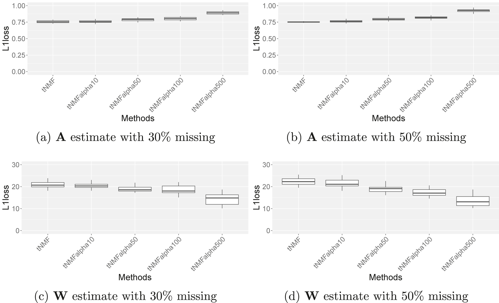
Four different values of α0 (10, 50, 100, and 500) were used for checking its effects, when the data is generated under the negative binomial model. As α0 gets larger, the W estimates become more accurate, whereas the A estimates are less accurate in both 30 and 50% missing rates.
A.3 Simulation study for using the log likelihood function for choosing K
We perform a simulation study to show how the likelihood method works for choosing a proper K under the simulation scenario of 3.2 with a zero-rate of 30%. Here, the true K is 3. From the likelihood method (Figure A.3.1), we are able to find K = 3 as the increase is reduced from K = 4.
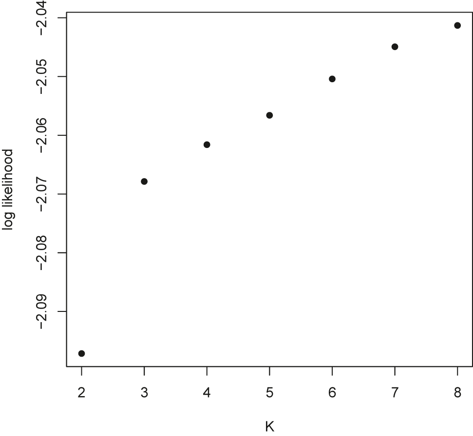
As K increases, the log-likelihood function increases. But the rate of increase is dropped when K = 4, hence we can infer K = 3 from the likelihood function.
References
1. Camp, JG, Badsha, F, Florio, M, Kanton, S, Gerber, T, Bräuninger, M, et al.. Human cerebral organoids recapitulate gene expression programs of fetal neocortex development. Proc Natl Acad Sci U S A 2015;112:15672–7. https://doi.org/10.1073/pnas.1520760112.Search in Google Scholar PubMed PubMed Central
2. Holmes, I, Harris, K, Quince, C. Dirichlet multinomial mixtures: generative models for microbial metagenomics. PloS One 2012;7:e30126. https://doi.org/10.1371/journal.pone.0030126.Search in Google Scholar PubMed PubMed Central
3. Sankaran, K, Holmes, SP. Latent variable modeling for the microbiome. Biostatistics 2019;20:599–614.10.1093/biostatistics/kxy018Search in Google Scholar PubMed PubMed Central
4. Gower, JC. Principal Coordinate Analysis. New York City: John Wiley & Sons; 2005.10.1002/0470011815.b2a13070Search in Google Scholar
5. Lee, DD, Seung, HS. Algorithms for non-negative matrix factorization. In: Advances in neural information processing systems. Cambridge, MA: MIT Press; 2001, vol 13:556–62 pp.Search in Google Scholar
6. Blei, DM, Ng, AY, Jordan, MI. Latent Dirichlet allocation. J Mach Learn Res 2003;3:993–1022.Search in Google Scholar
7. Alvarez, D, Hidalgo, H. Document analysis and visualization with zero-inflated poisson. Data Min Knowl Discov 2009;19:1–23. https://doi.org/10.1007/s10618-009-0127-4.Search in Google Scholar
8. Sohn, MB, Li, H. A GLM-based latent variable ordination method for microbiome samples. Biometrics 2017;74:448–57.10.1111/biom.12775Search in Google Scholar PubMed PubMed Central
9. Simchowitz, M, 2013. Zero-inflated Poisson factorization for recommender systems. Technical Report.Search in Google Scholar
10. Abe, H, Yadohisa, H. A non-negative matrix factorization model based on the zero-inflated tweedie distribution. Comput Stat 2017;32:475–99. https://doi.org/10.1007/s00180-016-0689-8.Search in Google Scholar
11. Zhu, L, Lei, J, Delvin, B, Roeder, K. A unified statistical framework for single cell and bulk RNA sequencing data. Ann Appl Stat 2018;12:609–32. https://doi.org/10.1214/17-aoas1110.Search in Google Scholar
12. Kharchenko, PV, Silberstein, L, Scadden, DT. Bayesian approach to single-cell differential expression analysis. Nat Methods 2014;11:740–2. https://doi.org/10.1038/nmeth.2967.Search in Google Scholar PubMed PubMed Central
13. Oh, J, Zhang, F, Doerge, R, Chun, H. Kernel partial correlation: a novel approach to capturing conditional independence in graphical models for noisy data. J Appl Stat 2018;45:2677–98. https://doi.org/10.1080/02664763.2018.1437123.Search in Google Scholar
14. Polson, NG, Scott, JG, Windle, J. Bayesian inference for logistic models using Polya-Gamma latent variables. J Am Stat Assoc 2013;108:1339–49. https://doi.org/10.1080/01621459.2013.829001.Search in Google Scholar
15. Owen, AB, Perry, PO. Bi-cross-validation of the SVD and the nonnegative matrix factorization. Ann Appl Stat 2009;3:564–94. https://doi.org/10.1214/08-aoas227.Search in Google Scholar
16. Anandkumar, A, Ge, R, Hsu, D, Kakade, SM, Telgarsky, M. Tensor decompositions for learning latent variable models. J Mach Learn Res 2014;15:2773–832.10.21236/ADA604494Search in Google Scholar
17. Kang, HJ, Kawasawa, YI, Cheng, F, Zhu, Y, Xu, X, Li, M, et al.. Spatio-temporal transcriptome of the human brains. Nature 2011;478:483–9. https://doi.org/10.1038/nature10523.Search in Google Scholar
18. Kozik, AJ, Nakatsu, CH, Chun, H, Jones-Hall, YL. Age, sex, and TNF associated differences in the gut microbiota of mice and their impact on acute TNBS colitis. Exp Mol Pathol 2017;103:311–19. https://doi.org/10.1016/j.yexmp.2017.11.014.Search in Google Scholar
19. Beals, E. Bray-curtis ordination: an effective strategy for analysis of multivariate ecological data. Adv Ecol Res 1984;14:55.10.1016/S0065-2504(08)60168-3Search in Google Scholar
20. Lozupone, C, Knight, R. UniFrac: a new phylogenetic method for comparing microbial communities. Appl Environ Microbiol 2005;71:8228–35. https://doi.org/10.1128/aem.71.12.8228-8235.2005.Search in Google Scholar
21. Wong, R, Wu, JR, Gloor, GB. Expanding the unifrac toolbox. PloS One 2016;11:e0161196. https://doi.org/10.1371/journal.pone.0161196.Search in Google Scholar PubMed PubMed Central
© 2021 Walter de Gruyter GmbH, Berlin/Boston
Articles in the same Issue
- Frontmatter
- Research Articles
- Integrating additional knowledge into the estimation of graphical models
- Asymptotic properties of the two one-sided t-tests – new insights and the Schuirmann-constant
- Bayesian optimization design for finding a maximum tolerated dose combination in phase I clinical trials
- A Bayesian mixture model for changepoint estimation using ordinal predictors
- Power prior for borrowing the real-world data in bioequivalence test with a parallel design
- Bayesian approaches to variable selection: a comparative study from practical perspectives
- Bayesian adaptive design of early-phase clinical trials for precision medicine based on cancer biomarkers
- More than one way: exploring the capabilities of different estimation approaches to joint models for longitudinal and time-to-event outcomes
- Designing efficient randomized trials: power and sample size calculation when using semiparametric efficient estimators
- Power formulas for mixed effects models with random slope and intercept comparing rate of change across groups
- The effect of data aggregation on dispersion estimates in count data models
- A zero-inflated non-negative matrix factorization for the deconvolution of mixed signals of biological data
- Multiple scaled symmetric distributions in allometric studies
- Estimation of semi-Markov multi-state models: a comparison of the sojourn times and transition intensities approaches
- Regularized bidimensional estimation of the hazard rate
- The effect of random-effects misspecification on classification accuracy
- The area under the generalized receiver-operating characteristic curve