Numerical Simulation of Inclusion Capture in the Slab Continuous Casting Considering the Influence of the Primary Dendrite Arm Spacing
-
Yanbin Yin
 ,
Shaowu Lei
,
Shaowu Lei

Abstract
In the present work, a coupled three-dimensional numerical model of fluid flow, heat transfer, and inclusion motion during the solidification of molten steel in slab continuous casting mold has been developed. Based on the model, this paper has studied the inclusion capture during the process. The influence of the primary dendrite arm spacing on inclusion capture has been considered. The inclusion distributions, total masses, and average diameters at different depth from the slab surface have been given out in the present paper. The simulation results revealed the inclusion concentration existed in the solidification process, and the inclusion capturing area varies with the depth from the slab surface.
Introduction
Large inclusion in the slab affects slab quality dramatically, especially for surface and mechanical property. In recent decades, researchers have developed many inclusion control technologies [1, 2], which can control inclusion content in steel at a low level. However, inclusions exist in steel inevitably, which are captured by the solidification front during solidification [3]. Besides, continuous casting mold is the last vessel which can remove inclusion from the steel. Therefore, it is necessary to research the inclusion behavior in continuous casting.
Extensive studies on continuous casting have been carried out by numerical simulation [4, 5, 6, 7, 8], which involve molten steel flow, heat transfer and mass transfer, and so on. For inclusion behavior, studies mainly focused on inclusion motion and floating removal [9, 10, 11, 13, 13] in continuous casting mold. However, these studies did not consider molten steel solidification almost. Nevertheless, the influence of molten steel solidification on molten steel flow and inclusion behavior is significant. So, it is necessary to study the inclusion behavior through coupling molten steel flow and solidification.
Scholars have presented a few papers [8, 14, 1516, 17] about inclusion behavior through coupling molten steel flow and solidification. Z. Liu et al. [15, 16] studied the transient turbulent flow, solidification, and transport and entrapment of particles in the continuous casting mold. The transient distribution of particles inside the liquid pool, the removal ratio, entrapment ratio, and escape ratio of particles were revealed. S. Lei et al. [8, 14], coauthors of this work, studied inclusion motion during the continuous casting slab solidification. Inclusion distributions and trajectories of different distance from the slab surface were given out. However, the primary dendrite arm spacing (PDAS) has an influence on inclusion capture [17]. The works mentioned above did not consider the influence of the PDAS. B.G. Thomas et al. [17] researched the influence of the PDAS on particle entrapment. Nevertheless, inclusion distribution in solidified continuous casting steel was not given out.
The present work has developed a three-dimensional coupled numerical model of molten steel flow, heat transfer, and inclusion capture, considering the influence of the PDAS. The enthalpy-porosity technique [18], which can couple the flow with heat transfer directly, was adopted in this work to simulate molten steel solidification. Inclusion capturing criterion developed by Y. Miki et al. [19] for evaluating inclusion capture was modified in this work through including the influence of the PDAS.
Numerical model
The numerical model consists of two parts: solidification and flow model, inclusion capture model. The solidification and flow model is a steady numerical model, which provides the initial condition for the inclusion capture model, such as temperature field, flow field, and the solidification shell distribution. Nevertheless, the inclusion capture model is a transient Lagrangian approach, which simulate the inclusion capture during molten steel solidification in the continuous casting mold.
Assumptions in this model
The following assumptions are included in the present numerical model:
The molten steel is considered as steady and incompressible Newton flow;
The fluctuation of molten steel and mold flux in mold is neglected;
The top surface thermal condition of mold is considered as thermal isolation;
The caster is perfectly vertical with respect to the gravitational field and the curvature of the strand is ignored;
The inclusions are spherical, whose density is 3500 kg/m3 constantly;
Inclusion collision is not considered. Since the inclusion volume fraction is extremely low relative to molten steel volume fraction, influence of inclusion on fluid flow and heat transfer is neglected;
Only the evolution of latent heat resulting from solid-liquid phase change is considered;
Fluid flow in the mushy zone submits Darcy’s law.
Inclusions capturing model
Basic conservation equations
The mass and momentum conservation equations take the follow forms:
where
The term
where
and
Enthalpy-porosity technique
The present work has adopted enthalpy-porosity technique [18] to simulate molten steel solidification, which treats the mushy region as a “pseudo” porous medium. A variable called the liquid fraction, which indicates the volume fraction of steel in liquid form, is computed for each cell in the simulation domain at each iteration. The liquid fraction,
where
The enthalpy of the steel,
where
The latent heat content can be written in terms of the steel latent heat,
where
where
In mushy zone, the porosity is equal to the liquid fraction. When the molten steel has fully solidified, the liquid fraction and porosity become zero simultaneously, and the velocity of solidified steel is equal to the casting speed. The influence of porosity on fluid flow velocities is dramatic, which can be introduced into the momentum conservation equation source term:
where
Particle force balance equation
The movement of the inclusions is governed by the particle force balance equation defined as follows:
where
Drag force can be described as:
where
The pressure gradient force [22] can be given as follows:
The buoyancy force [22] can be expressed as:
where
where
Saffman force [23], which is caused by the uneven velocity distribution of the velocity boundary layer, is derived according to formula as follows:
where
Suction force [24] derived from the concentration gradient is expressed as:
where
According to data collected by K. Mukai and W. Lin [25], the inclusion interfacial tension in molten steel can be written as:
hence,
In term of solidification theory proposed by M.C. Flemings [26], solute concentration in the boundary layer can be described as:
thus,
where
Turbulent dispersion of particles
The stochastic transport of particles (STP) [27] is adopted to describe dispersion of particles resulting from turbulence of molten steel flow. The STP model is based on established theories of stochastic process modeling.
where
PDAS-model
The present work has adopted the PDAS-Model, which was developed by M. El-Bealy and B.G. Thomas [28], to evaluate the PDAS. The model can be expressed as:
where
Geometry model of simulation domain
As Figure 1 shows, full geometry model has been developed, slab with a size of 0.25 m × 1. 6 m × 2 m is divided into cells of which the minimum and maximum sizes are 0.001 m and 0.01 m respectively. The submerged depth of the nozzle is 0.2 m, the nozzle inner diameter is 0.085 m. And the SEN port is rectangular, with a height of 0.075 m, width of 0.07 m and 15 degrees downward. As Figure 1(c) shows, for the sake of computing accuracy, the grid boundary layer has been refined.

A schematic view of the slab domain (a), mesh of slab cross section at 0.8 m from meniscus (b), and the enlarged view of the rectangular box in b (c).
Physical properties and boundary condition
Physical properties
Physical properties of molten steel are listed in Table 1.
Properties of steel and boundary condition.
| Parameters | Values | Dimensions |
|---|---|---|
| 0.7 | % | |
| 0.02 | % | |
| 1 × 10⁻⁴ [25] | ||
| 2.6 × 10⁻⁹ [25] | ||
| 0.02 [25] | 1 | |
| 700 | ||
| 31 | ||
| 7000 | ||
| 264000 | ||
| 1727 | ||
| 1673 | ||
| 0.0055 [7] | ||
| 0.02 | ||
| 1747 |
Boundary conditions
For nozzle inlet boundary condition, all variables were assumed to be constant. The inlet velocities of molten steel and inclusions are assumed to be identical, which are defined using the casting speed. Besides, the molten steel temperature at the nozzle inlet is equal to that in tundish, because temperature decline is negligible when molten steel flows from tundish to mold. All the variables mentioned above can be described as follows:
where
A fully developed boundary condition that normal gradients of all variables are set to be zero has been adopted at domain outlet [6].
According to the paper of P.J. Flint [4], an empirical formula has been used for heat flux through the middle of broad face, which can be described as follows:
where
Air gap exists between the mold wall and the solid shell near the slab corners, which may result in inconsistent distribution of heat flux in slab width direction. To deal with this problem, the present work has adopted the assumption that the heat flux decreases linearly from the middle of the slab broad face to the slab corner. And the heat flux at the corner is 80 pct of that in the broad face [4]. In the secondary cooling zone, thermal boundary condition can be described as follows [8]:
where
According to the experimental data, the inclusion size distribution at the mold inlet is illustrated in Figure 2.

Inclusion distribution at the mold inlet.
Results and discussion
Heat transfer and solidification
Figure 3 shows steel liquid fractions at different cross sections, which reveals that solidification shell is almost uniform at 0.1 m from the meniscus. Nevertheless, solidification shell gets uneven at 0.3 m from the meniscus. The inhomogeneity displays that solidification shell is thin at slab narrow face and its vicinity, on the contrary, it is thick at the slab broad face. The inhomogeneity of solidification increases with distance from the meniscus.

Liquid fractions at different slab cross sections: 0.1 m (a) 0.2 m (b) 0.3 m (c) 0.4 m (d) 0.5 m (e) 0.6 m (f) 0.7 m (g) 0.8 m (h) from the meniscus.
As Figure 4 shows, molten steel velocity distributions are also uneven at different cross sections. Velocities are larger near the inhomogeneous zones of solidification shell. Based on the results, the present work assumes the scour of molten steel results in the inhomogeneity of solidification shell.

Steel velocity distributions at different slab cross sections: 0.1 m (a) 0.2 m (b) 0.3 m (c) 0.4 m (d) 0.5 m (e) 0.6 m (f) 0.7 m (g) 0.8 m (h) from the meniscus.
Velocity and PDAS at the solidification front
According to the works of Y. Miki et al. [19] and W. Yamada [30], inclusion capture happens at the solidification front where the liquid fraction is less than 0.2 [19], which is a sufficient condition. Besides, only the inclusion size and molten steel velocity at the solidification front meet the requirements showed in Figure 5, can the inclusions be captured by the solidification front. As Figure 6 shows, in the present work, the max velocity of the molten steel at solidification front is 0.061 m/s. Besides, as Figure 2 shows, the max diameter of inclusions is 195 μm (1 μm = 1 × 10⁻⁶ m). It is obvious that all inclusions can be captured by the solidification front according to the criterion. The works of Y. Miki et al. [19] and W. Yamada [30] revealed the relationship between steel flow velocity and maximum diameter of inclusions. However, these works did not consider the effect of the PDAS on inclusion capture.

Relationship between the molten steel velocity and maximum diameter of the entrapped inclusion.

Molten steel velocity distribution at the solidification front.
As Figure 7(a) and (b) shows, the present paper assumes the solidification front cannot capture the inclusion whose diameter is larger than the local PDAS. In this case, the force which the PDAS exerts on the inclusion cannot offset the buoyancy. On the contrary, the solidification front can capture the inclusion whose diameter is smaller than the local PDAS.
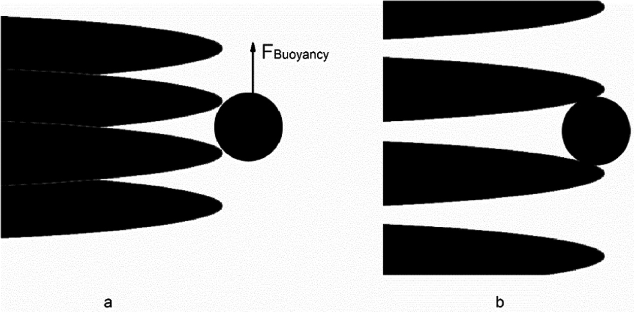
Schematic drawings of the solidification front capturing the inclusion: the local PDAS is less than the inclusion diameter (a) and larger than the inclusion diameter (b).
In the present work, the PDAS (in μm) has been calculated by the PDAS-Model. And the results reveal the differences of PDAS at solidification front are significant. As Figure 8 illustrates, the PDAS is lower than 170 μm at 0.2 m from the meniscus, which means the solidification front at this position cannot capture inclusions that are larger than 170 μm. Moreover, not all PDAS are larger than the largest inclusion size at 1 m from the meniscus. In other words, large inclusions cannot be captured by the solidification front at this position, considering that their diameters are larger than local PDAS.

PDAS of solidification front at different mold cross sections: 0.2 m (a) and 1 m (b) from the meniscus.
Because of the phenomenon mentioned above, in the present work, the inclusion capture criterion [19] have been modified by taking into account the influence of the PDAS.
Effect of the PDAS on inclusion distribution
The inclusion (in μm) distributions at different depths from the slab broad surface with capturing area(shadow zone) and sampling area(pattern zone) are shown in Figures 9 and 10. Figure 9 shows the results without considering the effect of the primary arm space, by contrast, Figure 10 shows the results considering the effect of the PDAS.

Inclusion distributions at different depths without considering the effect of the PDAS: 0~0.01 m from broad surface (a) 0.01~0.02 m from broad surface (b) 0.02~0.03 m from broad surface (c) 0.03~0.04 m from broad surface (d).

Inclusion distributions at different depths taking into account the effect of the PDAS: 0~0.01 m from broad surface (a) 0.01~0.02 m from broad surface (b) 0.02~0.03 m from broad surface (c) 0.03~0.04 m from broad surface (d).
As Figure 9 (b) and (c) show, at 0.01~0.03 m from the slab broad surface, the inclusions concentrate at the quarter of the slab broad face. Besides, inclusions whose sizes are larger than 100 μm concentrate at 0.00~0.03 m from the broad surface, as shown in Figure 9 (a), (b), and (c). As shown in Figure 9 (a), the inclusion capturing area at 0~0.01 m from the slab broad surface locates at 0.0~0.1 m from meniscus. As shown in Figure 9 (b), the inclusion capturing area at 0.01~0.02 m from the slab broad surface locates at 0.1~0.4 m from meniscus. Moreover, Figure 9 (c) and (d) show uneven distribution of the inclusion capturing area at 0.02~0.04 m from the slab broad surface. The pattern zone represents sampling area where simulation data about inclusion amounts, weights and sizes have been extracted.
As Figure 10 shows, the capturing areas are same as that in Figure 9. Similarly, at 0.01~0.03 m from the slab broad surface, the inclusions concentrate at the quarter of the slab broad face. And inclusions whose sizes are larger than 100 μm concentrate at 0.00~0.03 m from the broad surface.
Through comparing Figures 9 and 10, the amount of the inclusions captured by solidification shell is less in the PDAS-Model. Furthermore, as shown in Figure 10 (a), inclusions whose sizes are larger than 130 μm are not discovered at 0~0.01 m below the slab broad surface. As illustrated in Figure 10 (b), inclusions whose sizes are larger than 170 μm are not discovered at 0.01~0.02 m below the slab broad surface.
Figure 11 shows the PDAS of the inclusion capturing area at different depths from the slab surface. As Figure 11 (a) shows, PDAS is less than 130 μm at 0~0.01 m below the slab surface. As Figure 11(b) shows, PDAS is less than 170 μm at 0.01~0.02 m below the slab surface. These conditions lead to the results revealed in Figure 10 (a) and (b).

PDAS of the inclusion capturing area at different depths: 0~0.01 m from broad surface (a) 0.01~0.02 m from broad surface (b) 0.02~0.03 m from broad surface, (c) 0.03~0.04 m from the slab surface (d).
Discussion
The number, mass, and size of inclusions have been extracted from the sampling areas. The inclusion mass and average diameter are calculated as follows:
where

The relationships between the inclusion number (a), mass (b), average diameter (c) and the distance from the slab broad surface.
As Figure 8 (a) shows, the inclusion number in the PDAS-Model case at each position is slightly less than that in no PDAS-Model case. Nevertheless, for the inclusion mass and average diameter, there are significant differences between the two cases. As is shown in Figure 8 (b), for the two cases, the difference of the inclusion mass in sampling area at 0.01~0.02 m below the slab broad surface is the largest. As shown in Figure 8 (c), the difference of the inclusion average diameter in sampling area at 0~0.01 m below the slab broad surface is the largest. Since the influence of the PDAS on the inclusion capture cannot be neglected, the simulated data in the PDAS-Model case is less than that in the no PDAS-Model case generally.
Conclusions
The present work has investigated inclusion motion and capture during the solidification of the continuous casting slab. The inclusion distributions, total masses, and average diameters at different positions from the slab broad surface have been given out in the present paper.
The present work has modified the inclusion capturing criterion using the PDAS-Model. Basing on the modified criterion, the effect of the PDAS on the inclusion capture has been revealed. The conclusions can be drawn as follows:
The PDAS has an influence on the inclusion capture. The solidification front can capture inclusion whose diameter is less than the local PDAS, on the contrary, inclusion whose diameter is larger than the PDAS cannot be captured.
Inclusion concentration exists in solidification shell: at 0.01~0.03 m from the slab broad surface, the inclusions concentrate at the quarter of the slab broad face. And inclusions whose sizes are larger than 100 μm concentrate at 0.00~0.03 m from the broad surface.
The inclusion capturing area varies with the depth from the slab broad surface. At 0~0.01 m below the slab broad surface, the inclusion capturing area locates at 0.0~0.1 m from meniscus. At 0.01~0.02 m below the slab broad surface, the inclusion capturing area locates at 0.1~0.4 m from meniscus. At 0.02~0.04 m from the slab broad surface, the inclusion capturing areas distributes unevenly.
The influence of the PDAS on inclusion capture is significant at 0~0.02 m below the slab broad surface.
Funding statement: National Natural Science Foundation of China, (Grant / Award Number: ‘51474023’, ‘U1360201’).
Acknowledgments
The authors gratefully express their appreciation to the National Natural Science Foundation of China (U1360201) and (51474023) for sponsoring this work. Sincere gratitude and appreciation should be expressed to Professor Jiongming Zhang for his careful guidance.
References
[1] H.V. Atkinson and G. Shi, Prog. Mater Sci., 48 (2003) 457–520.10.1016/S0079-6425(02)00014-2Search in Google Scholar
[2] T. Matsumiya, ISIJ Int., 46 (2006) 1800–1804.10.2355/isijinternational.46.1800Search in Google Scholar
[3] H. Yasuda, I. Ohnaka and H. Jozuka, ISIJ Int., 44 (2004) 1366–1375.10.2355/isijinternational.44.1366Search in Google Scholar
[4] P.J. Flint, Proceedings of the 73rd Steelmaking Conference, Iron and Steel Society, Warrendale, PA (1990), pp. 731–744Search in Google Scholar
[5] S.K. Choudhary and D. Mazumdar, ISIJ Int., 34 (1994) 584–592.10.2355/isijinternational.34.584Search in Google Scholar
[6] S.H. Seyedein and M. Hasan, Int. J. Heat Mass Transfer, 40 (1997) 4405–4423.10.1016/S0017-9310(97)00064-1Search in Google Scholar
[7] X. Huang and B.G. Thomas, Can. Metall. Q., 37 (1998) 197–212.10.1179/cmq.1998.37.3-4.197Search in Google Scholar
[8] S. Lei, J. Zhang, X. Zhao and K. He, ISIJ Int., 54 (2014) 94–102.10.2355/isijinternational.54.94Search in Google Scholar
[9] L. Zhang, Y. Wang and X. Zuo, Metall. Mater. Trans. B, 39 (2008) 534–550.10.1007/s11663-008-9154-6Search in Google Scholar
[10] [10] M.D. Santis and A. Ferretti, ISIJ Int., 36 (1996) 673–680.10.2355/isijinternational.36.673Search in Google Scholar
[11] H. Lei, D.Q. Geng and J.C. He, ISIJ Int., 49 (2009) 1575–1582.10.2355/isijinternational.49.1575Search in Google Scholar
[12] [12] L. Zhang, J. Aoki and B.G. Thomas, Metall. Mater. Trans. B, 37 (2006) 361–379.10.1007/s11663-006-0021-zSearch in Google Scholar
[13] [13] L.T. Wang, Q.Y. Zhang, S.H. Peng and Z.B. Li, ISIJ Int., 45 (2005) 331–337.10.2355/isijinternational.45.331Search in Google Scholar
[14] [14] S. Lei, J. Zhang, X. Zhao and Q. Dong, Trans. Indian Inst. Metals, 69 (2016) 1193–1207.10.1007/s12666-015-0665-ySearch in Google Scholar
[15] Z. Liu, B. Li, L. Zhang and G. Xu, ISIJ Int., 54 (2014) 2324–2333.10.2355/isijinternational.54.2324Search in Google Scholar
[16] Z. Liu, L. Li, B. Li and M. Jiang, JOM, 66 (2014) 1184–1196.10.1007/s11837-014-1010-3Search in Google Scholar
[17] B.G. Thomas, Q. Yuan, S. Mahmood, R. Liu and R. Chaudhary, Metall. Mater. Trans. B, 45 (2014) 22–35.10.1007/s11663-013-9916-7Search in Google Scholar
[18] A.D. Brent, V.R. Voller and K.J. Reid, Numerical Heat Transfer, 13 (1988) 297–318.10.1080/10407788808913615Search in Google Scholar
[19] Y. Miki, H. Ohno, Y. Kishimoto and S. Tanaka, Tetsu-to-Hagané, 97 (2011) 423–432.10.2355/tetsutohagane.97.423Search in Google Scholar
[20] B.E. Launder and D.B. Spalding, Lectures in Mathematical Models of Turbulence, Academic Press, Salt Lake City, (1972).Search in Google Scholar
[21] C.T. Crowe, J.D. Schwarzkopf, M. Sommerfeld and Y. Tsuji, Multiphase Flows with Droplets and Particles, 2nd Edition, Crc Press, Florida, (2011).10.1201/b11103Search in Google Scholar
[22] N. Bessho, R. Yoda, H. Yamasaki, T. Fujii, T. Nozaki and S. Takatori, ISIJ Int., 31 (1991) 40–45.10.2355/isijinternational.31.40Search in Google Scholar
[23] P. Saffman, J. Fluid Mech., 22 (1965) 385–400.10.1017/S0022112065000824Search in Google Scholar
[24] K. Mukai and W. Lin, Tetsu-to-Hagané, 80 (1994) 527–532.10.2355/tetsutohagane1955.80.7_527Search in Google Scholar
[25] K. Mukai and W. Lin, Tetsu-to-Hagané, 80 (1994) 533–538.10.2355/tetsutohagane1955.80.7_533Search in Google Scholar
[26] M.C. Flemings, Solidification Processing, McGraw-Hill, New York, (1974).10.1007/BF02643923Search in Google Scholar
[27] L.L. Baxter and P.J. Smith, Energy Fuels, 7 (1993) 852–859.10.1021/ef00042a022Search in Google Scholar
[28] M. El-Bealy and B.G. Thomas, Metall. Mater. Trans. B, 27 (1996) 689–693.10.1007/BF02915668Search in Google Scholar
[29] K.Y.M. Lai, M. Salcudean, S. Tanaka and R.I.L. Guthrie, Metall. Trans. B, 17 (1986) 449–459.10.1007/BF02670209Search in Google Scholar
[30] W. Yamada, Curr. Adv. In Mater. Processes, 12 (1999) 682–684.Search in Google Scholar
© 2018 Walter de Gruyter GmbH, Berlin/Boston
This article is distributed under the terms of the Creative Commons Attribution Non-Commercial License, which permits unrestricted non-commercial use, distribution, and reproduction in any medium, provided the original work is properly cited.
Articles in the same Issue
- Frontmatter
- Research Articles
- Effect of Heat Treatment on Microstructure and Thermal Fatigue Properties of Al-Si-Cu-Mg Alloys
- Effect of Laser Welding Parameters on Weld Bowing Distortion of Thin Plates
- Effect of the Tundish Gunning Materials on the Steel Cleanliness
- Effects of Laser Shock Processing on Impact Toughness of Ti-17 Titanium Alloy
- Effect of Prior Thermomechanical Treatment on Annealed Microstructure and Microhardness in Cobalt-Based Superalloy Co-20Cr-15W-10Ni
- Oxidation Resistance of Austenitic Steels under Thermal Shock Conditions in an Environment Containing Water Vapor
- Comparative Evaluation of Spark Plasma and Conventional Sintering of NiO/YSZ Layers for Metal-Supported Solid Oxide Fuel Cells
- Present Situation and Prospect of EAF Gas Waste Heat Utilization Technology
- Formation of Nano-porous Structure in a Cathode at the Interface between Pt Electrode and YSZ during CO2 Electrolysis at 1,000 °C
- Numerical Simulation of Inclusion Capture in the Slab Continuous Casting Considering the Influence of the Primary Dendrite Arm Spacing
- Effect of Surface Fe-Sn Intermetallics on Oxide Films Formation of Stainless Steel in High Temperature Water