Numerical Modeling of Fluid Flow, Heat Transfer and Arc–Melt Interaction in Tungsten Inert Gas Welding
-
Linmin Li
 ,
Lichao Liu
,
Lichao Liu

Abstract
The present work develops a multi-region dynamic coupling model for fluid flow, heat transfer and arc–melt interaction in tungsten inert gas (TIG) welding using the dynamic mesh technique. The arc–weld pool unified model is developed on basis of magnetohydrodynamic (MHD) equations and the interface is tracked using the dynamic mesh method. The numerical model for arc is firstly validated by comparing the calculated temperature profiles and essential results with the former experimental data. For weld pool convection solution, the drag, Marangoni, buoyancy and electromagnetic forces are separately validated, and then taken into account. Moreover, the model considering interface deformation is adopted in a stationary TIG welding process with SUS304 stainless steel and the effect of interface deformation is investigated. The depression of weld pool center and the lifting of pool periphery are both predicted. The results show that the weld pool shape calculated with considering the interface deformation is more accurate.
Introduction
Tungsten inert gas (TIG) welding has been widely used in welding operations because of the considerable precision and a high level of weld quality. Deep understanding of the process mechanism related to the thermo-physical phenomena is of great significance for process optimization and practical application. The interactions of electric, magnetic, fluid dynamic, thermal effects, and the strong nonlinear thermodynamic and transport properties of arc plasma make it difficult to completely model the process. Particularly, the melt convection and interface deformation that induced by the interaction between arc and weld pool would significantly affect the melt dynamics and final pool shape [1–3]. Taking account of all these phenomena is necessary for the numerical model development.
Modeling of the arc plasma and weld pool has been concerned for a long time. In the past few decades, numbers of researchers [4–7, 10–17] have been working on modeling of arc welding processes, meanwhile, have acquired great progresses. Hsu et al. [5] early reported a series of comprehensive data of temperature, current density, pressure, etc. in a free burning argon arc by both experiment and numerical simulation. The calculated temperature fields and the essential results of different cases were in good agreement with the measurements. Evans and Tankin [8] measured the radiation of an argon plasma and Liu [9] provided the properties of argon with the varying temperatures. The argon plasma properties have been used in several numerical modeling works [2, 10–13]. To combine the arc and weld pool, Tanaka et al. [1] treated the tungsten cathode, arc plasma and anode as a unified model. The effect of different driving forces on weld pool shape was investigated, but the effect of arc–pool interface deformation was not considered. They also mentioned that the interface deformation was important as it should change the interfacial forces. The effect of driving forces, especially the Marangoni force, on the weld pool was also investigated by numbers of researchers [14–20]. A review of predictions of weld pool profiles was carried out by Tanaka and Lowke [21]. To consider the effect of arc–weld pool interface deformation, Choo et al. [22] simulated the TIG welding arc and weld pool by postulating a given interface shape. Kim et al. [23] investigated the effect of anode surface deformation on arc properties using a fitted surface boundary, the weld pool was not taken into account. Lei et al. [24] simulated the united TIG welding arc and weld pool with considering the free surface deformation under arc pressure and gravity using the surface deformation model proposed by Kim et al. [25]. In this model, only the depression of weld pool surface was simulated. Later on, Lu et al. [2] used a similar method to investigate the effect of interface deformation. Besides, the weld pool surface was always assumed flat in previous works.
Recently, Chakraborty [26] investigated the effects of turbulence on the molten pool transport, and Kim and Lee [27] investigated the turbulence effects on the arc plasma transport. More accurate results were obtained but the impacts were limited. Wang et al. [28] used the unified mathematical model to investigate the arc plasma and weld pool in double electrodes TIG welding. Jian et al. [11] employed the volume of fluid (VOF) method to track the keyhole boundary in keyhole plasma arc welding (PAW) process. Tashiro et al. [29] clarified the fume formation mechanism in TIG welding theoretically through numerical analysis.
The arc–pool interface deformation is important to interfacial forces, pool shape and final weld quality. A comprehensive representation of the free surface phenomena could play an important role in providing greatly improved insight into weld pool behaviors and could represent an interesting frontier in the modeling of arc welding systems [22]. The main purpose of the present work is to take the interface deformation into account to develop a united model with two-way coupling between the transport phenomena in arc and weld pool. Firstly, the model for welding arc is presented for a free burning arc. The calculated temperature fields and the essential results are validated against the experimental data [5]. Then the unified model without interface deformation is adopted to simulate a TIG welding process of a stainless steel SUS304 which has a negative temperature coefficient of surface tension. The drag, Marangoni, buoyancy and electromagnetic forces are respectively investigated and validated. Finally, all the driving forces are taken into account and an interface deformation model is incorporated using the dynamic mesh technique for interface tracking. The smoothing method is used because the interface is not severely deformed in TIG welding [11]. The unsteady simulation of the process using the present model with dynamic coupling is achieved and the effect of interface deformation on final pool shape is investigated.
Model formulation
Figure 1 shows a schematic representation of welding arc and pool for a stationary TIG welding operation. The arc is struck between cathode and anode to melt the workpiece. The interface between arc and weld pool should be deformed due to the arc–melt interactions. In the present work, the system is assumed to be axisymmetric. The magnetohydrodynamic (MHD) equations are incorporated into the finite volume method (FVM) based software FLUENT and solved using user defined scalars (UDS) and user defined functions (UDF). To simulate the interface deformation, an algorithm using the dynamic mesh technique is implemented according to the pressure balancing between the two sides of interface, and the smoothing method, which updates the position of each node on the interface and deforms the domain mesh in conjunction with the moving interface nodes, is used. The following assumptions are also made:
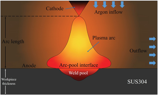
Schematic diagram of TIG welding process.
The flow of arc plasma is under atmospheric pressure. The plasma properties are temperature dependent as shown in Figure 2.
The arc plasma is a continuum and in local thermodynamic equilibrium (LTE).
The metal vapor from the anode surface is neglected and the surface tension linearly decreases with increasing temperature.
The Boussinesq approximation is used to handle the thermal buoyancy in weld pool without considering the solute buoyancy.
![Figure 2: Thermophysical properties [8, 9] of argon plasma for calculations.](/document/doi/10.1515/htmp-2016-0120/asset/graphic/htmp-2016-0120_figure2.gif)
Governing equations
Based on the above assumptions, the governing equations used to describe the heat transfer and fluid flow can be expressed as follows. One set of conservation equations is used for the whole domain, but different thermodynamic and transport parameters, as well as the source terms, are used in different zones.
Equation of mass continuity:
Conservation of radial momentum:
Conservation of axial momentum:
where the gravity in weld pool is expressed as:
When the anode surface deformation is taken into account, the shear stress direction changes to the face parallel direction.
The enthalpy-porosity method [30] with the Carman-Kozeny relation is used to model the anode melting. The radial and axial momentum source terms are respectively added in the weld pool to stop the flow in solidified zones according to the liquid fraction
where
where
The solution for temperature is essentially an iteration between the energy equation and the liquid fraction equation. The method for updating the liquid fraction can be found in the work by Voller and Swaminathan [30]. The Joule heating is considered in both arc and weld pool regions, but the additional source term S is different in the two regions. In arc region, it is calculated as:
The radiation loss
where L is the latent heat.
In order to calculate the electromagnetic force acting on the arc plasma and weld pool. The electromagnetic field is defined by Maxwell equations:
where
where
Boundary conditions and numerical details
The calculation domain with mesh is shown in Figure 3. Two cases of the distance between cathode tip (AB) and anode surface (HE) are used in the present work. For simulations of the free burning arc, the distance (AH) is kept at 10 mm, the anode melting is not considered. For simulations with anode melting of the welding process with a SUS304 stainless steel, the distance (AH’) is kept at 5 mm, the anode surface is changed to H’E’ and the simulation time is 20 s as the previous work [1].
Calculation domain and mesh.
The boundary conditions are specified in Table 1 with reference to Figure 3. The temperature of boundary CD is set to 1000 K for the first case [5] and 300 K for the second case [1] according to the previous works. For the centerline AG, the axial symmetry condition is used. The current density boundary condition is set on the cathode tip (AB) and the value is calculated according to the current and cathode tip area:
Boundary conditions.
| AB | BC | CD | DE | EF | FG | |
|---|---|---|---|---|---|---|
| 1 atm | 1 atm | |||||
| T | 3,000 K | 3,000 K | const. | 3,00 K | 3,00 K |
Note:
The dynamic mesh technique is adopted for the interface deformation solution. The movement of nodes on the weld pool surface are mutative and handled by a UDF. The smoothing method is adopted to solve the domain mesh deformation in conjunction with the moving nodes. The interface node updating model is developed according to Newton’s second law. The node position is updated and the pressure field is recalculated in every time step, so the pressure balancing between the two sides of interface will be achieved. The displacement of node
where
Physical parameters and material (SUS304) properties.
| Parameters | Value |
|---|---|
| Boltzmann constant (J/K) | 1.38×10⁻²³ |
| Electron charge (C) | 1.6×10⁻¹⁹ |
| Permeability of vacuum (H/m) | 4π×10–7 |
| Density (kg/m3) | 7,200 |
| Viscosity (kg/m/s) | 0.006 |
| Liquidus temperature (K) | 1,727 |
| Solidus temperature (K) | 1,670 |
| Specific heat (J/kg/K) | 600 |
| Thermal conductivity (W/m/K) | 20 |
| Latent heat (J/kg) | 245,000 |
| Surface tension temperature gradient (N/m/K) | –4.6×10⁻⁴ |
| Electric conductivity (S/m) | 770,000 |
Results and discussion
Simulations of welding arc
In order to validate the numerical model for arc, the cases of free burning arc are firstly simulated. The distance between cathode and anode is 10 mm (AH=10 mm) and the anode melting is not considered. The experimental data of Hsu et al. [5] is used for validation. Two current conditions, I=100 A and I=200 A, are solved and boundary conditions are specified the same as that in Hsu et al. [5]. Figure 4 shows the calculated temperature fields of the two conditions ((a) I=100 A, (b) I=200 A) and compares the predicted temperature contours with the experimental data. It is shown that the predicted arc temperature fields are in fairly good agreement with the experimental data. A typical bell shape of arc is predicted, as the strong cathode jet will impinge on the anode surface and change the direction. The highest temperatures of the two conditions have reached 17,000 K for I=100 A and 21,000 K for I=200 A respectively.
![Figure 4: Calculated temperature contours in comparison with the experimental data [5] at (a) 100 A and (b) 200 A.](/document/doi/10.1515/htmp-2016-0120/asset/graphic/htmp-2016-0120_figure4.jpg)
Calculated temperature contours in comparison with the experimental data [5] at (a) 100 A and (b) 200 A.
Figure 5 shows the streamlines and pressure fields under the two conditions in arc region. It can be found that gas is entrained from its surroundings by the electromagnetic pumping force in the cathode region and then enters the arc core. As the gas approaches the anode, it is forced to turn to radial direction and the strong cathode jet impinging on the anode causes the pressure on anode surface increased. Meanwhile, the velocity decreases with increasing the distance from cathode. As seen in the figure, the pressure at the cathode tip reaches about 500 Pa for I=100 A and, for I=200 A, it reaches about 900 Pa. On the other hand, the pressures at the center of anode surface are above 29 Pa and 257 Pa, and the maximum velocities reach 170 m/s and 280 m/s respectively under the two conditions.
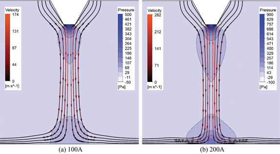
Pressure and fluid flow fields in arc region at (a) 100 A and (b) 200 A.
The variations of pressure, velocity, electrical potential and temperature along the axis of the two conditions ((a-b) I=100 A, (c-d) I=200 A) are plotted in Figure 6. It is seen that the velocity increases rapidly to the maximum velocity under the action of Lorentz force and then decreases to zero with increasing the distance to the cathode tip. The velocity drops sharply near the anode especially under the condition of I=200 A. At the cathode tip, a high pressure is also established by the electromagnetic force and decreases rapidly. In front of the anode, a pressure increment is resulted from the impingement of cathode jet on anode surface. Moreover, the calculated electrical potentials along the axis respectively increase from about –14 V and –12 V to 0 V, more rapidly near the cathode tip. The temperature also shows a rapid increment in front of the cathode, and as the arc spreads, the temperature drops over the arc region. The highest temperatures under the two conditions are about respectively 19,000 K and 23,000 K. The essential results including maximum temperature and axial velocity, voltage drop, and pressure at the cathode tip and at the center of anode surface are compared in Table 3. The results also show good agreement indicating that the present model for the welding arc is credible.
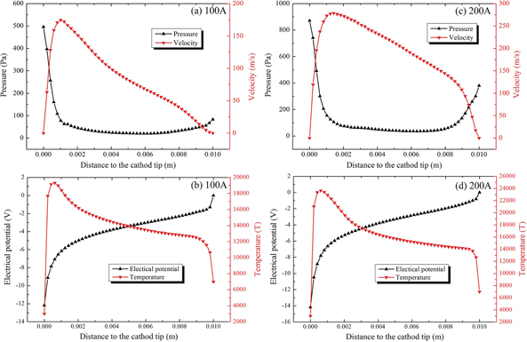
Variation of pressure, velocity, electrical potential and temperature along the axis of arc region.
The unified model
Secondly, the anode melting is considered and the weld pool is unified with the arc model. The distance between the cathode tip and anode surface is changed to 5 mm (AH’=5 mm). The current equal to 150 A, the properties of SUS304 for anode region and the simulation time of 20 s are adopted according to the work of Tanaka et al. [1] as well as the boundary conditions. To validate the driving forces (including drag force, buoyancy, electromagnetic force and Marangoni force) in weld pool and investigate the effect of each force on the pool shape, these four forces are separately added to the momentum equation in weld pool region. The interface deformation is not considered in this section. Figure 7 displays the fluid flow, temperature field and weld pool shape with respectively considering (a) drag force, (b) buoyancy, (c) electromagnetic force and (d) Marangoni force. The calculations are under the same condition. The results show that the drag force and Marangoni force (with a negative temperature coefficient of surface tension) are the main outward driving forces in weld pool. Furthermore, the buoyancy drives the melt downward in solidification front and leads to a clockwise flow while the electromagnetic force leads to an anticlockwise flow. The calculated maximum velocities are 44.3, 1.8, 4.3 and 20.5 cm/s respectively with the four forces. They agree well to the results of Tanaka et al. [1] which are respectively 47, 1.4, 4.9 and 18 cm/s. In this condition (I=150 A, AH’=5 mm), the maximum velocity in the arc (205 m/s) is also in fairly good agreement with the previous results [1, 31].
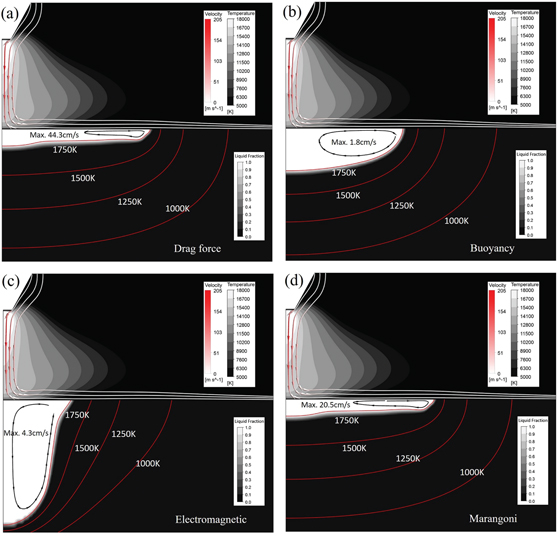
Fluid flow, temperature field and weld pool shape with different driving forces: (a) drag, (b) buoyancy, (c) electromagnetic force and (d) Marangoni force.
Then the drag, buoyancy, electromagnetic and Marangoni forces are all taken into account to calculate the final weld pool shape. Figure 8 shows the (a) current and Joule heating distributions, and (b) temperature and Lorentz force distributions. It is shown that the current density and the Joule heating are very high near the cathode tip. In front of the anode surface, an increment of current and Joule heating, which is because of the temperature distribution and the temperature dependent electrical conductivity, is found. The Lorentz force is found pointing to the arc core and continuously entrains the plasma from its surroundings. Besides, the highest temperature near the cathode tip reaches 17,700 K. Figure 9 is the temperature field and weld pool shape calculated by the unified model without interface deformation. The temperature field is compared with the result of the previous work [1], and a fairly good agreement can be seen. The comparison of weld pool shape between calculation and experiment (I=150 A, t=20 s) is shown in Figure 10. The calculated maximum velocity in weld pool is 49.8 cm/s. The radius of weld pool reaches about 8 mm. Though the predicted velocity and the weld pool shape are close to the calculation results of Tanaka et al. [1], the radius of the predicted weld pool is unacceptable larger than the experimental result, which is also found in Tanaka et al. [1]. The present work is going to investigate the effect of interface deformation on the weld pool shape.
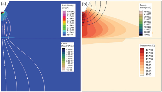
(a) Current density and Joule heating, (b) Lorentz force and temperature fields of the unified model.
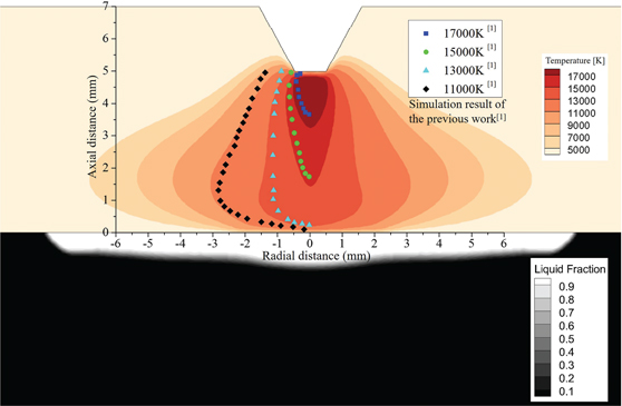
Weld pool shape and validation of temperature field.
Predictions considering interface deformation
As the interface deformation is important to the prediction of weld pool shape, the present work employs the above mentioned dynamic mesh interface deformation model to develop an arc–pool dynamic coupling model for process simulations. The condition is the same as that used in the previous section and all the driving forces are taken into account. Figure 11 depicts the temperature and pressure fields, and the weld pool shape with showing the deformed mesh. The temperature field is similar to the result without interface deformation, indicating that the interface deformation has a limited influence on the arc temperature distribution. The maximum pressure on the weld pool surface is about 200 Pa and leads to a depression in the center of weld pool. Besides, on the periphery of weld pool, the pool surface is lifted because of the impact of outward flowing melt on the solidification front. Figure 12 shows the comparison between the weld pool shape predicted by the coupled model with interface deformation and the experimental one. Compared with the result without considering the interface deformation, the maximum velocity is reduced to 38.5 cm/s and the weld pool radius is also reduced from about 8 mm to 6 mm, which is because the interface fluctuation will consume the outward momentum. The result shows that the model without interface deformation will bring about an unreasonable weld pool shape. Moreover, though the width of weld pool predicted by the model with interface deformation is more accurate, the pool depth still does not match the experiment. The reason may be that only the horizontal Marangoni force is considered but the vertical Marangoni force is not taken into account. Future work is needed to overcome this problem.
![Figure 10: Weld pool shapes of (a) simulation without interface deformation and (b) experiment [1].](/document/doi/10.1515/htmp-2016-0120/asset/graphic/htmp-2016-0120_figure10.jpg)
Weld pool shapes of (a) simulation without interface deformation and (b) experiment [1].
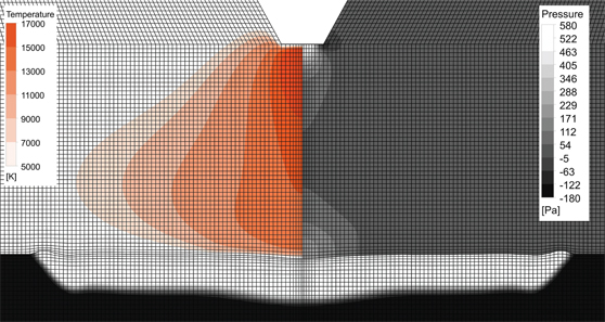
Temperature profile, pressure field and weld pool shape predicted by the dynamic coupled model with interface deformation.
![Figure 12: Comparison of weld pool shape between (a) simulation with interface deformation and (b) experiment [1].](/document/doi/10.1515/htmp-2016-0120/asset/graphic/htmp-2016-0120_figure12.jpg)
Comparison of weld pool shape between (a) simulation with interface deformation and (b) experiment [1].
Conclusions
A new model that includes the arc–weld pool dynamic coupling is developed on basis of magnetohydrodynamic (MHD) equations and an interface deformation model implemented using the dynamic mesh technique. Some conclusions can be summarized as follows:
For simulations of free burning arc, the temperature fields and essential results predicted by the present model are compared with both experimental and numerical results of Hsu et al. [5], and fairly good agreements are obtained.
The arc–weld pool unified model is employed to a stationary TIG welding process with stainless steel SUS304. The driving forces including drag, buoyancy, electromagnetic and Marangoni forces are considered, and their effects on the weld pool convection are respectively investigated and validated. Reliable flow fields in both arc and weld pool regions are predicted.
The dynamic mesh method is successfully implemented into the unified model to simulate the process with considering the interface deformation and investigate its effect on the weld pool shape. The depression of weld pool center and the lifting of pool periphery are predicted. It is also found that the model without interface deformation will bring about an unreasonable weld pool shape. A more credible weld pool shape is predicted by the present model with interface deformation.
Funding statement: Authors are grateful to the National Natural Science Foundation of China for support of this research, Grant No. U1508214.
References
1. K.C. Hsu, K. Etemadi and E. Pfender, J. Appl. Phys., 54 (1983) 1293–1301.10.1063/1.332195Suche in Google Scholar
2. V.R. Voller and C.R. Swaminathan, Numer. Heat Transfer B., 19 (1991) 175–189.10.1080/10407799108944962Suche in Google Scholar
3. T. Sandor, C. Mekler, J. Dobranszky and G. Kaptay, Metall. Mater. Trans. A, 44 (2013) 351–361.10.1007/s11661-012-1367-2Suche in Google Scholar
4. Y.L. Xu, Z.B. Dong, Y.H. Wei and C.L. Yang, Theor. Appl. Fract. Mech., 48 (2007) 178–186.10.1016/j.tafmec.2007.05.004Suche in Google Scholar
5. Y.J. Kim and J.C. Lee, J. Korean Phys. Soc., 62 (2013) 1252–1257.10.3938/jkps.62.1252Suche in Google Scholar
6. R.T.C. Choo and J. Szekely, Weld. J., 71 (1992) 77s-93s.Suche in Google Scholar
7. D.L. Evans and R.S. Tankin, Phys. Fluids, 10 (1967) 1137–1144.10.1063/1.1762256Suche in Google Scholar
8. R.T.C. Choo, J. Szekely and R.C. Westhoff, Metall. Trans. B, 23 (1992) 357–369.10.1007/BF02656291Suche in Google Scholar
9. S.P. Lu, H. Fujii and K. Nogi, Sci. Technol. Weld. Join, 9 (2004) 272–276.10.1179/136217104225012346Suche in Google Scholar
10. N. Chakraborty, Appl. Therm. Eng., 29 (2009) 3618–3631.10.1016/j.applthermaleng.2009.06.018Suche in Google Scholar
11. Y. Lei, X. Gu, Y. Shi and H. Murakawa, Acta Metall. Sin.,37 (2001) 537–542.Suche in Google Scholar
12. I. Egry, High Temp. Mater. Processes, 22 (2003) 303–308.10.1515/HTMP.2003.22.5-6.303Suche in Google Scholar
13. W. Dong, S. Lu, D. Li and Y. Li, Int. J. Heat Mass Transfer, 54 (2011) 1420–1431.10.1016/j.ijheatmasstransfer.2010.07.069Suche in Google Scholar
14. M. Tanaka, H. Terasaki, M. Ushio and J.J. Lowke, Metall. Mater. Trans. A, 33 (2002) 2043–2052.10.1007/s11661-002-0036-2Suche in Google Scholar
15. S.P. Lu, H. Fujii and K. Nogi, Metall. Mater. Trans. A, 35 (2004) 2861–2867.10.1007/s11661-004-0234-1Suche in Google Scholar
16. S. Tashiro, T. Zeniya, K. Yamamoto and K. Suzuki, J. Phys. D Appl. Phys., 43 (2010) 801–804.Suche in Google Scholar
17. X. Jian and C.S. Wu, Int. J. Heat Mass Transfer, 84 (2015) 839–847.10.1016/j.ijheatmasstransfer.2015.01.069Suche in Google Scholar
18. X. Wang, D. Fan, J. Huang and Y. Huang, Int. J. Heat Mass Transfer, 85 (2015) 924–934.10.1016/j.ijheatmasstransfer.2015.01.132Suche in Google Scholar
19. X. Wang, J. Gong, Y. Zhao, Y. Wang and Z. Ge, High Temp. Mater. Processes, 35 (2016) 121–128.10.1515/htmp-2014-0170Suche in Google Scholar
20. C.F. Liu, Ph.D. Thesis, University of Minnesota, Minneapolis, MN (1977).Suche in Google Scholar
21. J. Hu and H.L. Tsai, Int. J. Heat Mass Transfer, 50 (2007) 833–846.10.1016/j.ijheatmasstransfer.2006.08.025Suche in Google Scholar
22. W.H. Kim, H.G. Fan and S.J. Na, Numer. Heat Transfer Part A, 32 (1997) 633–652.10.1080/10407789708913910Suche in Google Scholar
23. C.V. Goncalves, S.R. Carvalho and G. Guimaraes, Appl. Therm. Eng., 30 (2010) 2396–2402.10.1016/j.applthermaleng.2010.06.009Suche in Google Scholar
24. M. Goodarzi, R. Choo and J.M. Toguri, J. Phys. D Appl. Phys., 31 (1998) 569–583.10.1088/0022-3727/31/5/014Suche in Google Scholar
25. J. Hu, H. Guo and H.L. Tsai, Int. J. Heat Mass Transfer, 51 (2008) 2537–2552.10.1016/j.ijheatmasstransfer.2007.07.042Suche in Google Scholar
26. S.C. Snyder and R.E. Bentley, J. Phys. D Appl. Phys., 29 (1996) 3045–3049.10.1088/0022-3727/29/12/017Suche in Google Scholar
27. W.H. Kim, H.G. Fan and S.J. Na, Metall. Mater. Trans. B, 28 (1997) 679–686.10.1007/s11663-997-0042-2Suche in Google Scholar
28. M. Tanaka and J.J. Lowke, J. Phys. D Appl. Phys., 40 (2007) R1-R23.10.1088/0022-3727/40/1/R01Suche in Google Scholar
29. Y.T. Cho and S.J. Na, Int. J. Precis. Eng. Man., 16 (2015) 787–795.10.1007/s12541-015-0104-3Suche in Google Scholar
30. H. Fujii, T. Sato, S.P. Lu and K. Nogi, Mater. Sci. Eng. A, 495 (2008) 296–303.10.1016/j.msea.2007.10.116Suche in Google Scholar
31. F. Lu, X. Tang, H. Yu and S. Yao, Comput. Mater. Sci., 35 (2006) 458–465.10.1016/j.commatsci.2005.03.014Suche in Google Scholar
© 2017 Walter de Gruyter GmbH, Berlin/Boston
This article is distributed under the terms of the Creative Commons Attribution Non-Commercial License, which permits unrestricted non-commercial use, distribution, and reproduction in any medium, provided the original work is properly cited.
Artikel in diesem Heft
- Frontmatter
- Editorial
- Preface to the Special Issue on “Cutting Edge of Computer Simulation of Solidification, Casting and Refining”
- Review Article
- Recent Aspects on the Effect of Inclusion Characteristics on the Intragranular Ferrite Formation in Low Alloy Steels: A Review
- Research Articles
- Numerical Simulation and Experimental Casting of Nickel-Based Single-Crystal Superalloys by HRS and LMC Directional Solidification Processes
- Dendrite Growth Characteristics and Segregation Control of Bearing Steel Billet with Rotational Electromagnetic Stirring
- Deformation and Structure Difference of Steel Droplets during Initial Solidification
- Research on Soft Reduction Amount Distribution to Eliminate Typical Inter-dendritic Crack in Continuous Casting Slab of X70 Pipeline Steel by Numerical Model
- Effect of Composition, High Magnetic Field and Solidification Parameters on Eutectic Morphology in Cu-Ag Alloys
- Processing and Microstructure Characteristics of As-Cast A356 Alloys Manufactured via Ultrasonic Cavitation during Solidification
- Mathematical Modeling on Deformation Behavior of Solidified Shell in Continuous Slab Casting with Soft Reduction
- Effect of Construction Manner of Mould Cluster on Stray Grain Formation in Dummy Blade of DD6 Superalloy
- Review Article
- Application of Mathematical Models for Different Electroslag Remelting Processes
- Research Articles
- Numerical Modeling of Fluid Flow, Heat Transfer and Arc–Melt Interaction in Tungsten Inert Gas Welding
- Analysis of Power Supply Heating Effect during High Temperature Experiments Based on the Electromagnetic Steel Teeming Technology