Ground volume assessment using ’Structure from Motion’ photogrammetry with a smartphone and a compact camera
-
Rafał Wróżyński
 ,
Mariusz Sojka
,
Mariusz Sojka

Abstract
The article describes how the Structure-from-Motion (SfM) method can be used to calculate the volume of anthropogenic microtopography. In the proposed workflow, data is obtained using mass-market devices such as a compact camera (Canon G9) and a smartphone (iPhone5). The volume is computed using free open source software (VisualSFMv0.5.23, CMPMVSv0.6.0., MeshLab) on a PCclass computer. The input data is acquired from video frames. To verify the method laboratory tests on the embankment of a known volume has been carried out. Models of the test embankment were built using two independent measurements made with those two devices. No significant differences were found between the models in a comparative analysis. The volumes of the models differed from the actual volume just by 0.7‰ and 2‰. After a successful laboratory verification, field measurements were carried out in the same way. While building the model from the data acquired with a smartphone, it was observed that a series of frames, approximately 14% of all the frames, was rejected. The missing frames caused the point cloud to be less dense in the place where they had been rejected. This affected the model’s volume differed from the volume acquired with a camera by 7%. In order to improve the homogeneity, the frame extraction frequency was increased in the place where frames have been previously missing. A uniform model was thereby obtained with point cloud density evenly distributed. There was a 1.5% difference between the embankment’s volume and the volume calculated from the camera-recorded video. The presented method permits the number of input frames to be increased and the model’s accuracy to be enhanced without making an additional measurement, which may not be possible in the case of temporary features.
1 Introduction
In the last 20 years, we have been able to observe a dynamic development in the area of geomatics [1, 2]. The classic geodesic measurement methods which were used to obtain topographic data are slowly being replaced by automated photogrammetric and laser measurements. Terrestrial laser scanning (TLS) and airborne laser scanning (ALS) are now used on a large scale to acquire data [3, 4]. The data obtained in these ways are used in many scientific fields e.g. in geomorphology [5–11], archaeology [3, 12–17], ecology [18–23] and engineering [24–26]. Data acquired by the laser scanning are characterised by high resolution and accuracy and can be used to create the surface models of the studied features. One of the principal applications is creating three-dimensional Digital Surface Models (DSMs) and Digital Terrain Models (DTMs). Obtaining data using laser scanning techniques requires expensive equipment and often a specialist software. Laser scanners are designed to make measurements easy and almost automatic. Additionally, specialist commercial software dedicated for these applications can be used to easily process the data and then visualise it or build a numerical model of the studied features. This saves a lot of time spent on obtaining, processing and analysing the data, but these solutions are very expensive. Solutions of this kind have unquestionable advantages of technical support from hardware and software manufacturers and instruction manuals. SfM [1], a measurement method originating from computer vision techniques which have been gaining popularity and is not very expensive [1, 27–30, 32], seems to be the next step in terrain data acquisition. This method is based on the same tenets as stereoscopic photogrammetry, but so far it has been rarely used for the field measurements [1, 12, 32–34]. In the SfM method, 3D structures are created from a series of an overlapping frame (Fig. 1).
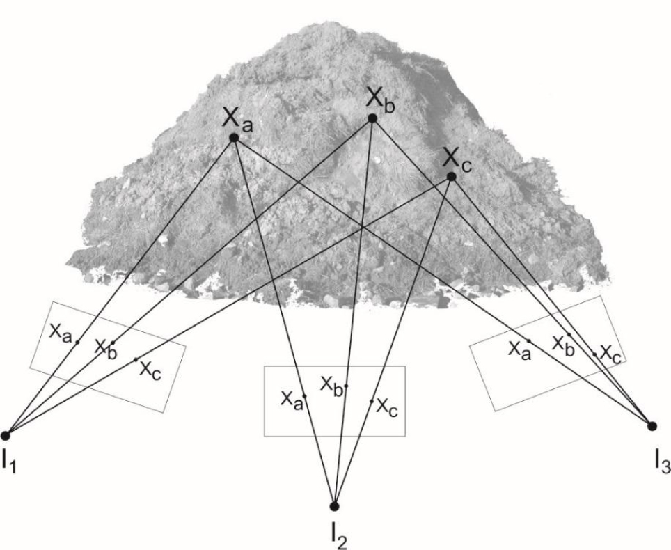
SfM diagram
The fundamental difference between stereoscopic photogrammetry and the SfM method is that the calculations necessary to obtain a precise location of a point in three-dimensional space are made fully automatic and precise positioning of the cameras is not necessary. Additionally, it is possible to use video recording, as the change in the camera’s orientation does not influence the reconstruction of points in space. This allows the complete three-dimensional structure of the observed scene to be captured. SfM also uses a highly redundant, iterative bundle adjustment procedure, based on a database of features automatically extracted from multiple overlapping images [35]. To the date, modelling has mostly been based on still image sets [12, 29, 32]. The necessary condition is to use sets of photos with a high cover rate. At present several cloud-processing engines are used, the best-known of which are the following commercial programs: Microsoft Photosynth [1] PhotoModeler [12] and Agisoft Photoscan [28, 36] and free software e.g. Bundler [28] and VisualSFM [37]. These programs use bundle adjustment in the final phase of point position determination to minimise reprojection errors between the photograph and the anticipated point position. Bundle adjustment seeks to minimise a geometric cost function (e.g., the sum of squared reprojection errors) by jointly optimising both the camera and point parameters using non-linear least squares [38, 39]. The point-cloud generated using SfM algorithms is relative and must be calibrated to actual dimensions. Such calibration is carried out using several known ground-control points (GCPs). GCPs should be clearly marked in order to be easily identified against the background of the studied object and the distances between them should be known. SfM is more and more commonly used in scientific research because it is, first of all, a low-cost method. Devices used in everyday life such as digital cameras, camcorders or smartphones with cameras as well as free software and home computers can be used in this method. However, it must be noted that more time and, more importantly, better skills are necessary to acquire and process the data. Yet, improvements to non-commercial software dedicated for such applications that have been observed in recent years allow even non-specialists to build three-dimensional models of features which are subjects of scientific research. Wide access to discussion panels which provide significant informal technical support is also of importance.
Tarolli [40] predicted that, in a few years time, to create accurate high-resolution DEMs or DSMs for any application, users will use a simple smartphone camera. Three-dimensional numerical terrain models can be constructed from videos recorded with popular mobile phones, cameras or camcorders. Fonstad et al. [41] indicate that SfM may be useful not only from a cost-savings and ease-of-construction perspective. Carrivick et al. [42] suggest that SfM workflow has significantly more automation and thus is perceived by users as being much more straightforward and simple than photogrammetry. This ease of use has been greatly enhanced in recent years by the development of freely available software. Gienko and Terry [43] show that 3D models created in this way can serve as an accurate and reliable representation of the real objects and that the methodology is advantageous for efficient and precise measurement. Results obtained by Javernick et al. [44] suggest that low-cost, logistically simple SfM method can deliver high-quality terrain datasets competitive with those obtained with significantly more expensive laser scanning, and suitable for geomorphic change detection and hydrodynamic modelling. Westoby et al. [1] compared a SfM derived DEM with a similar model obtained using terrestrial laser scanning and suggested that decimetre-scale vertical accuracy can be achieved using SfM also in areas with complex topography. Golparvar-Fard et al. [45] demonstrated that in laboratory and field experiments, the accuracy of using the image-based point cloud models is slightly less than the point cloud generated by the laser scanner, while both approaches allow the as-built environment to be visualised from different viewpoints. Fonstad et al. [41] showed that the SfM method helps avoid the problems of shadowing and drop-outs common to terrestrial and aerial laser scanning. This article shows how research on micro-topography (100 to 104 mm) of anthropogenic origin can be carried out using SfM.
1.1 Goal of this article
The goal of this article was to show how a low-cost SfM method can be used to calculate the volume of anthropogenic micro-topography. The usability of the SfM method was tested by making measurements using two independent devices: a smartphone (iPhone 5) and a camera (Canon G9) in the laboratory and in the field. Automatically extracted video frames, recorded with a smartphone and a camera, was used to create a 3D model. This demonstrates that equipment used in everyday life (a digital camera and a smartphone) can be used to make measurements in the field and free software can be used to build a Three-dimensional model and to calculate the volume. The research showed the versatility of the SfM method as independent measurement conditions (different recording devices and users) allows obtaining reliable results.
2 Methods
The usefulness of SfM for calculating micro-topography volume was tested in this work. The workflow was divided into four stages (Fig. 2). In the first stage, data acquisition was described. Next, the method of the preliminary data selection (preprocessing) was presented. The third stage included a detailed description of the method of building the DSM using the SfM (processing). In the fourth stage, the methods of model calibration and microtopography volume calculation were presented (postprocessing). Additionally, the results obtained in laboratory measurements using a smartphone and a camera were compared. Finally, the proposed method was tested on the embankment in the field.
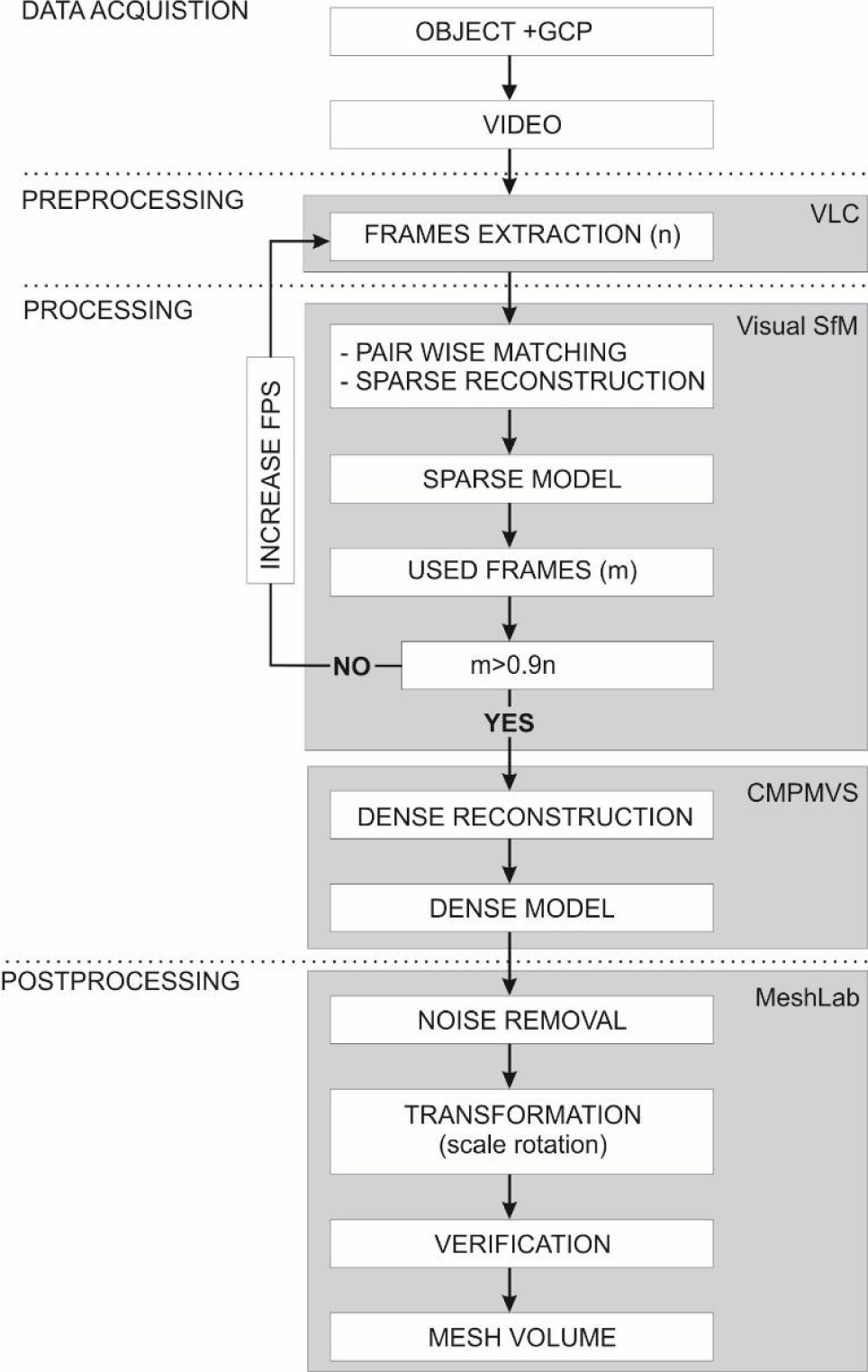
Workflow of the proposed volume measurement method
2.1 Data acquisition
In the laboratory, an embankment was formed from 3000 cm3 of soil of 0.063<d ≤ 2.0 mm granulation. Volume changes due to the possible consolidation of soil were omitted as the irrelevant small values. Two pairs of GCPs were marked around the embankment. The distance between point pairs 1-2 and 3-4 was 200 mm (Fig. 3a). Then, the embankment was filmed using a smartphone and a camera making sure the GCPs were visible. The aim of using independent measurements taken by two independent people with two different recording devices was to check if the method is universal. Table 1 contains detailed technical characteristics of the equipment used.
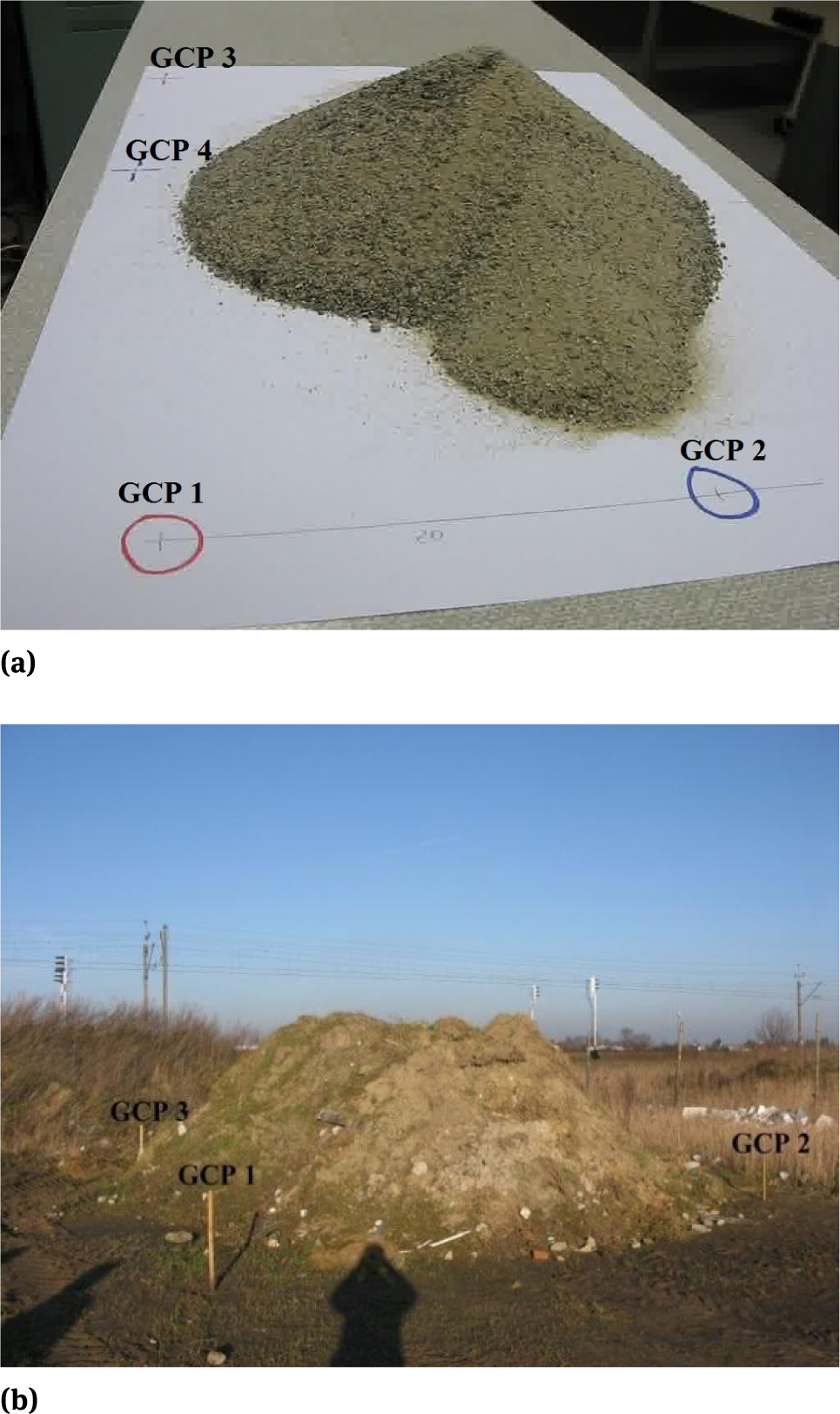
Laboratory test embankment (a), field embankment (b) with GCPs marked
Technical parameters of the devices used in field measurements
| Canon G9 | iPhone 5 | |
|---|---|---|
| Sensor type | CCD | CMOS |
| ChargeCoupled Device | Complementary Metal Oxide Semiconductor | |
| Sensor size | 12.1 Megapixels with a 1/1.7″ | 8.0 Megapixels with a 1/3.2″ |
| (~7.53 x 5.64 mm) sensor | (~4.5 x 3.37 mm) sensor | |
| Movie resolution | 1024x768 | 1920x1080 |
| Movie frame rate | 15 | 30 |
| Video format | AVI [M-JPEG] | MOV [H.264/ MPEG-4 AVC] |
| Pixelsize | 1.87 μm | 1.4 μm |
| Diagonal | 9.41 mm | 5.62 mm |
| Focal length | 7.40 mm | 4.12 mm |
| SurfaceArea | 42.47 mm2 | 15.17 mm2 |
| Aspect Ratio | 16:9 | 16:9 |
The test results are presented in Table 2.
Input data and the characteristics of the built models
| Test 1 | Test 2 | Model 1 | Model 2a | Model 2b | |
|---|---|---|---|---|---|
| Camera | Canon G9 | iPhone5 | Canon G9 | iPhone5 | iPhone5 |
| Movie length (s) | 151 | 201 | 89 | 99 | 99 |
| Frames | 151 | 201 | 89 | 99 | 161 |
| Frame resolution | 1024×768 | 1920×1080 | 1024×768 | 1920×1080 | 1920×1080 |
| Used frames | 151 | 201 | 87 | 85 | 160 |
| Computation time (min) | 57 | 118 | 37 | 63 | 103 |
| Vertices | 828 055 | 2 387 750 | 1 043 579 | 2 453 744 | 2 798 390 |
| Model vertices | 301 096 | 618 108 | 632 516 | 1 352 245 | 1 303 230 |
| Density [p/cm2] | 267 | 539 | 0.9 | 1.9 | 1.8 |
| Volume [cm3] | 2994.46 | 2998.93 | 3.028·107 | 2,863·107 | 3.076·107 |
After successful laboratory assessment of the SfM method for building DSM using video frames acquired with everyday devices, the measurements were made in the field in the same way. A small artificial building embankment was selected. Four GCPs (Fig. 3b) were established around the embankment and then the distances between them were measured with a tape (0.5 cm accuracy). Then the embankment was filmed, while making sure the GCPs were visible. The recordings were 88 and 95 seconds in duration, respectively on the camera and smartphone.
2.2 Preprocessing
In the second stage, the videos from camera and smartphone were copied to a computer. Then, using the VLC media player software (v2.1.3) frames were automatically extracted, with one frame per second (fps) frequency. All the calculations were made using a standard personal computer with the following parameters: Intel(R) Core(TM) i7-3370k CPU with 8GB RAM and Nvidia GeForce GTX 650Ti graphic card.
2.3 Processing
In the third stage, the frames were loaded to VisualSFM. VisualSFM is a GUI application for 3D reconstruction using SfM [37]. Feature detection and full pairwise matching were performed and then sparse reconstruction was carried out. Dense reconstruction was carried out in CMPMVS v.0.6.0 [46], which is a multi-view reconstruction software. The input to this software is a set of perspective images and camera parameters (internal and external camera calibrations) which were imported from VisualSFM software. In this way, a dense model of the embankment in the form of a point cloud and textured mesh in the .ply and .wrl formats was obtained. DSM of the embankment made in the laboratory was created using VisualSFM (v0.5.23) and CMPMVS (v0.6.0), called Test 1 (smartphone) and Test 2 (camera). Using the same methodology DSM of the embankment measured in the field were made and called Model 1 (smartphone) and Model 2 (camera).
2.4 Postprocessing
In the fourth stage, the embankment models, as a point-cloud from CMPMVS, were processed using the MeshLab (v1.3.2) software [47]. The points identified as reflections from adjacent objects were discarded. The filtered point-clouds were calibrated in MeshLab using the scale and rotate function on the basis of the GCPs. The first GCP pair (12) was used for scaling purpose and second GCP pair (3-4) for verification. When building DSM of embankments only for the purpose of calculating the volume, it is not necessary to use full georeference. A transform from a relative local reference system to an absolute and correctly scaled reference system was undertaken. Volume of the embankment was calculated in MeshLab software using the calibrated model.
2.5 Statistical analysis
The open-source CloudCompare (v2.5) software was used to compare the created models. CloudCompare is an application for managing and comparing 3D point-clouds and surface meshes [48]. CloudCompare was used to calculate the differences between the dense point-clouds models. CloudCompare uses Hausdorff distance to calculate the differences [49]. The program can also be used to calculate the basic statistics (min, max and mean distance, standard deviation, distribution fitting: Gauss and Weibull). The differences between the models obtained using CloudCompare were exported to the .txt format and detailed statistical analysis in the Statistica 10 software was made. The differences between the models were presented in the box- and-whisker plot, where the median, 25% and 75% quartile values as well as the range of non-outlying values were shown. Then the set of differences was assessed in terms of the presence of outlying and extreme values by means of the 3-sigma rule. The distributions of differences between the models was tested using the K-S test. The distribution of the outlying and extreme values was analysed. The two-dimensional spherical analysis was used for this purpose. The spherical analysis was made in 36 sections of an identical width of 10 degrees. For each section the following basic statistical parameters were calculated: the maximum, minimum and mean values, the median and the standard deviation. The significance of the differences between the mean values in the next sections was assessed using the F test.
3 Results
The input data used to create DSMs are shown in Table 2. The lengths of films recorded using smartphone and camera were 201 and 150 seconds respectively. The film imported from a smartphone was converted from the Quick Time (.mov) format to the (.avi) format. The videos recorded with the camera were recorded in the .avi format. Frames with the .jpg extension were extracted from both films, with the resolution of 1920×1080 for smartphone and 1024×768 for a camera. Then the collections of frames were loaded into VisualSfM and using the image matching and sparse reconstruction function preliminary sparse models of the embankments were made. The analysis of the number of frames used to build the models from these pre-selected ones showed that all of them were useful (Fig. 4). Therefore, it is not necessary to increase the frequency of extraction from the videos.
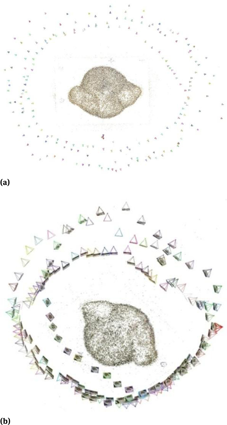
Camera poses computed with VisualSFM Test 1 (a) and Test 2 (b)
In the next stage, the models were dense reconstructed in the CMPMVS software. The dense models Test 1 and Test 2 contained 82.8 104 and 23.8 105 points respectively. The difference between the number of points making up the models resulted mainly from the number of frames used and frame resolution (Table 2). This also affected the computing time necessary to build the DSM, 57 and 118 minutes respectively. The result is a fully Three-dimensional model of the embankment in the form of a point cloud and textured mesh (Fig. 5).
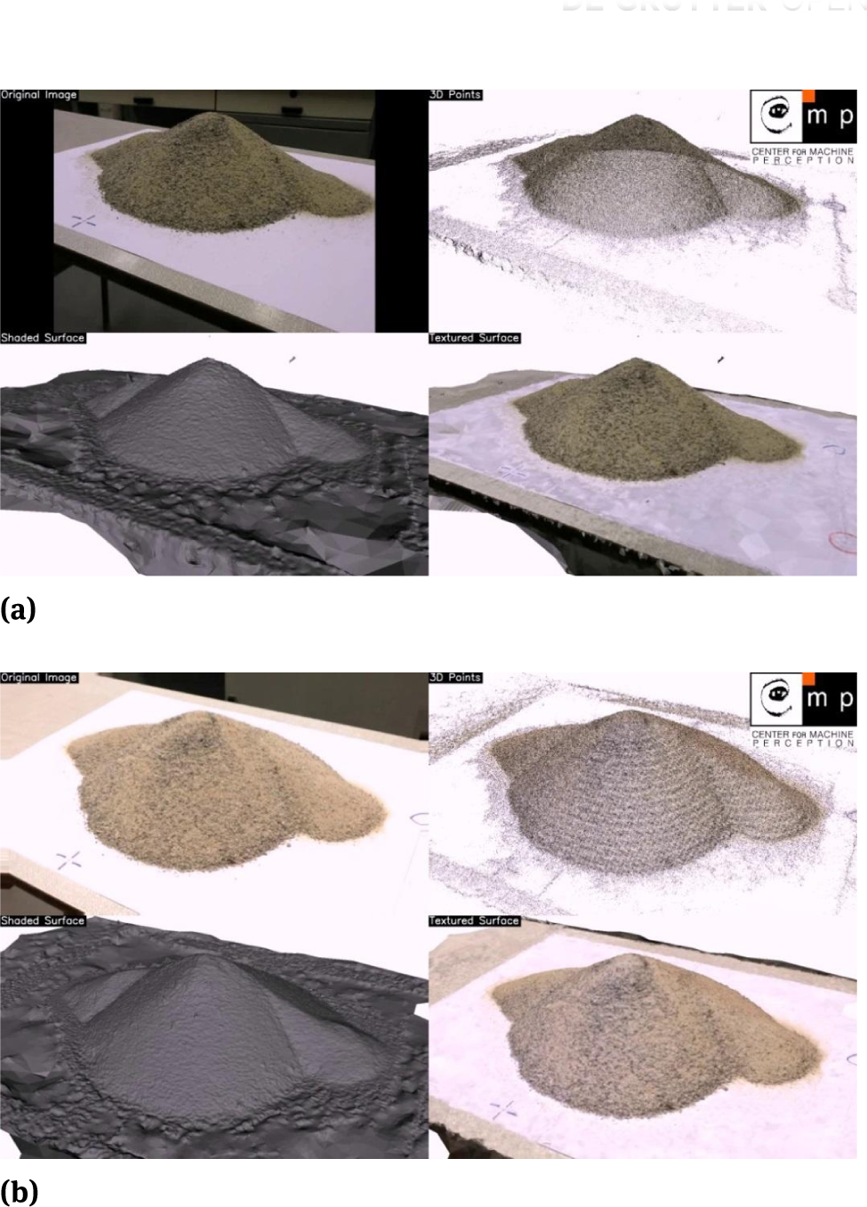
Dense reconstructed model Test 1 (a) and Test 2 (b) - original image, 3D points, shaded surface and textured surface.
Test 1 and Test 2 models were imported to the MeshLab software, where they were turned and re-scaled for the model transformation. The excess data, reflections from adjacent objects, were removed from the models. 63% of the points were removed from the Test 1 model and 74% from the Test 2. The density of the points making up the Test 2 was approximately twice as high as the Test 1 model. The parameters of both models are shown in Table 2. Then, the volumes of Test 1 and Test 2 models were computed using MeshLab. The analysis showed that the models obtained with different devices and by independent users were similar. The volumes of the embankments were 2994 cm3 and 2998 cm3 for the models respectively. These values were very similar to the volume of soil originally used in the lab, the difference was 2‰ and 0.7‰ respectively. In order to verify the quality of the models, the point clouds were exported from MeshLab to CloudCompare. The clouds were compared and the differences between models were computed (Fig. 6).
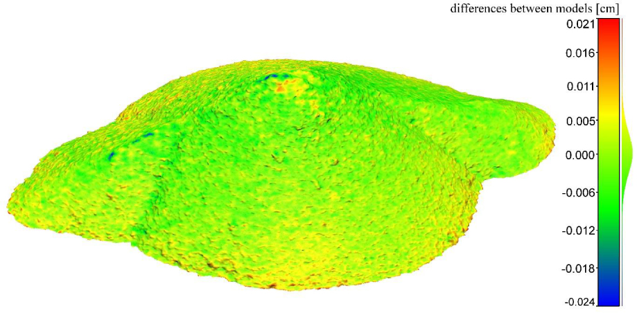
The distribution of differences calculated with CloudCompare (Test 1 minus Test 2)
The results from CloudCompare were exported to the .txt format for statistical analysis in the STATISTICA software. A total of 61.8 104 differences were obtained, shown in a box-and-whisker plot. The differences between the models varied from −2.32 mm to 2.08 mm with the median value of 0.03 mm (Fig. 7a). The differences were assessed in terms of the presence of outlying and extreme values and 10,714 outlying and extreme points, 1.7% of the analysed dataset, were discarded. The outlying observations were marked with dots and the extreme values with crosses on Fig. 7b. It was observed that the greatest differences between the studied models appeared mainly at the bottom of the embankment. A spatial presentation of the outlying and extreme values permits the analysed embankment outline to be reconstructed. The analysis showed that the correspondence of the distribution of the differences in the normal distribution was at the level of 0.05 (Fig. 7c). The differences between Test 1 and Test 2 models were analysed at 10 degrees resolution (Fig. 7d) with the mean difference between the models close to the 0 value. The F test showed that there were no significant differences between mean values. It can be assumed, therefore, that the models built are uniform and the SfM method can be successfully used to create DSM of embankments.
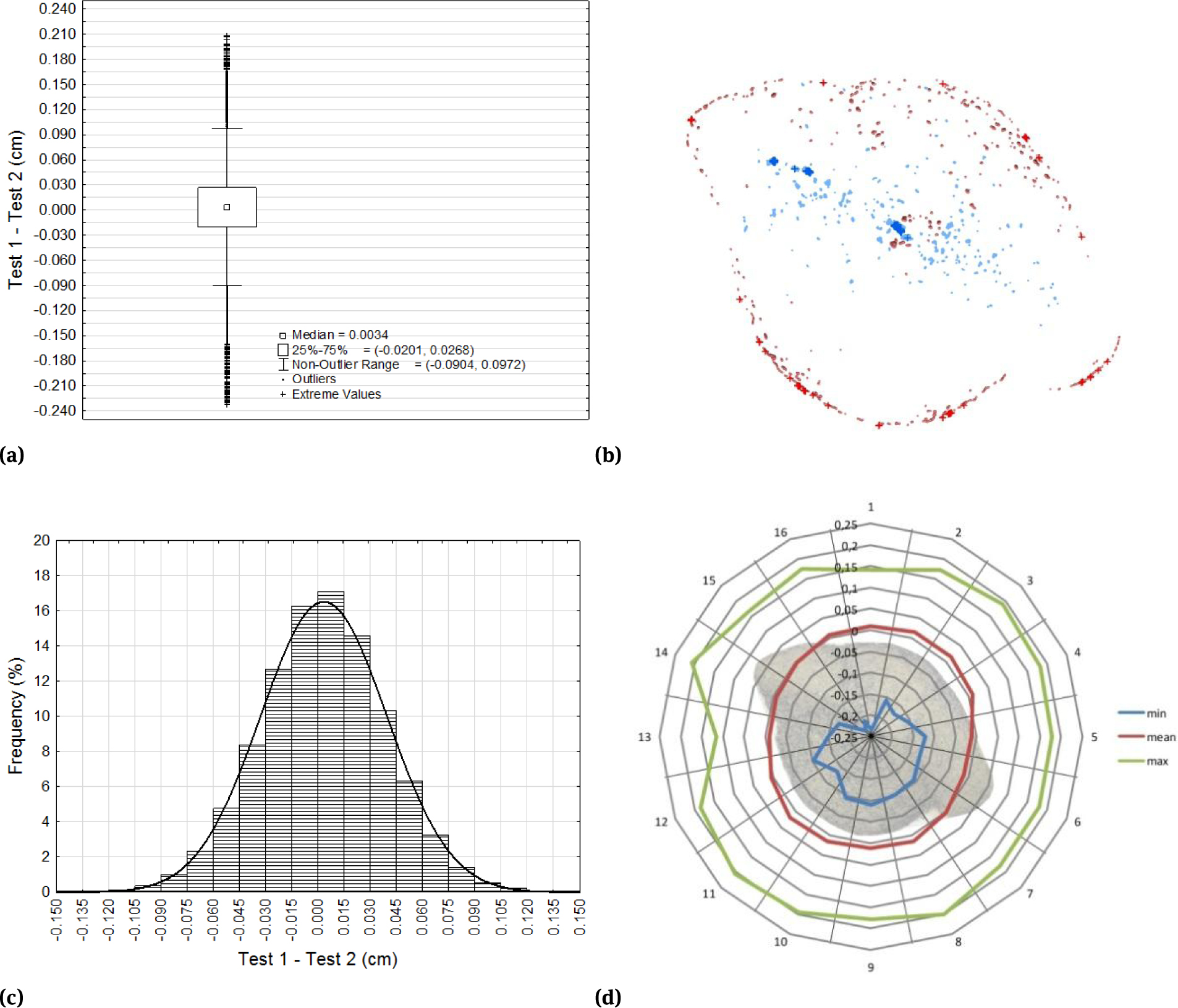
Differences between Test 1 and Test 2 models: box-and-whisker plot (a), distribution of outlying and extreme values (b), histogram (c), and the distribution of minimum, maximum and mean values in sections (d)
3.1 Field tests
Based on field measurement and using the same methods, two models were built. The preliminary verification of the sparse models showed that 87 and 85 extracted frames were used respectively. Only 2% (Fig. 8a) of the pre-selected frames were discarded from the video recorded with a camera and as much as 14% from the video made with a smartphone (Table 2). The quantity of discarded frames exceeded 10% of those pre-selected. Consequently, the model was thoroughly verified. It was observed that all the frames were discarded in one place (Fig. 8b), which was characterised by the greatest degree of shading when taking the measurement. As the sparse model was created, it was called Model 2a and then dense-reconstructed and used for further calculations. In order to improve the uniformity and quality of the model created with a smartphone, in the area where frames were discarded, their extraction frequency was increased to 3 fps. Thanks to the analysis of the results from VisualSfM and the available video from a smartphone, it was easy to locate and select a place from which additional frames could be extracted. A set of 161 new frames was thereby acquired, which was re-imported to VisualSfM. The model built in this way was called Model 2b (Fig. 8c) and was verified.
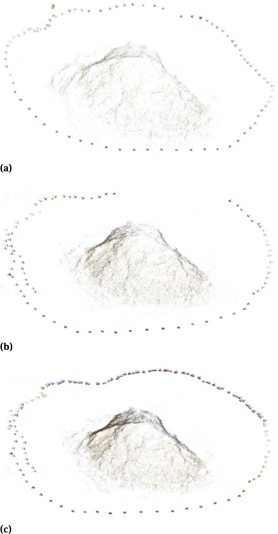
Camera poses computed with VisualSFM Model 1(a), Model 2a (b), Modl 2b (c)
The verification showed that 160 frames out of the 161 were used to build it. Then Model 1 (Fig. 9a), Model 2a (Fig. 9b) and Model 2b (Fig. 9c) were dense-reconstructed in CMPMVS.
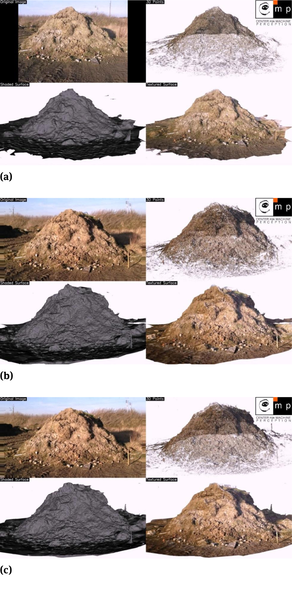
Dense reconstructed Model 1 (a), Model 2a (b), Model 2b (c) - original image, 3D points, shaded surface and textured surface
The model construction times in CMPMVS are shown in Table 2. The number of frames used to build the models and the resolution affected quantity of points which made up the dense models. Model 1 was created using 10.43 105 points while Model 2a and Model 2b contained more than twice that number – 24.5105 and 27.9105 respectively. Thus created dense models in the form of a point cloud were processed and calibrated in MeshLab. The set of points for Model 1 was reduced by 39% while those for Model 2a and Model 2b were reduced by 45% and 53% respectively. Model 2a had the highest density of the points making up the three-dimensional embankment model – 19.03103 p·m−2, for Model 2b the density was slightly lower – 18.08 103 p·m−2, and Model 1 had the lowest density of 9.13 103 p·m−2. The MeshLab computed embankment volume value ranged from 28.63 m3 for Model 2a to 30.76 m3 for Model 2b. The volume of the Model 1 embankment was 30.28 m3. The differences in the computed volumes between the embankments created using the whole frame set (Model 1 and Model 2a) were only 1.5%, and the volume of the Model 2a embankment differed by 7%. However, a decision was made to assess what impact the number of frames discarded during model creation in VisualSfM had on the uniformity and quality of the models. To do that the point clouds were compared in CloudCompare. The highest correspondence was obtained between Model 1 and Model 2b (Fig. 10b). The differences between these models had a normal distribution and ranged from −0.1 m to 0.1 m. Slightly larger differences were obtained for Model 1 and Model 2a (Fig. 10a) and Model 2a and Model 2b (Fig. 10c).
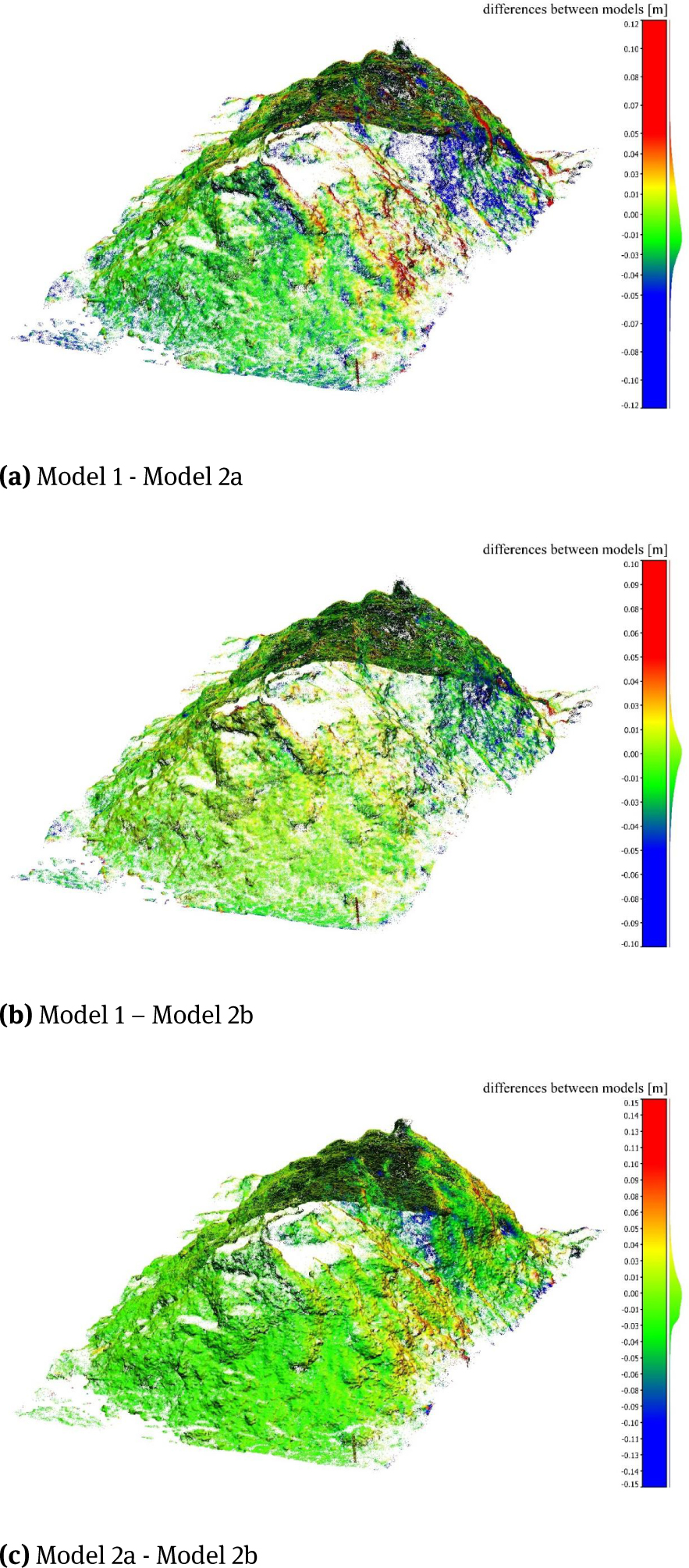
Distribution of differences between point clouds generated with CloudCompare
The difference distributions were other than normal, which may indicate that there exist local non-homogenous areas in the analysed models. Models 2a and 2b were analysed, especially the place where most frames had been discarded (Fig. 11a). It was observed that a large number of discarded frames in this place influenced the point cloud volume in the dense models. (Fig. 11b). The volume of the points making up Model 2a was clearly lower in the analysed area than in Model 2b (Fig. 11c).
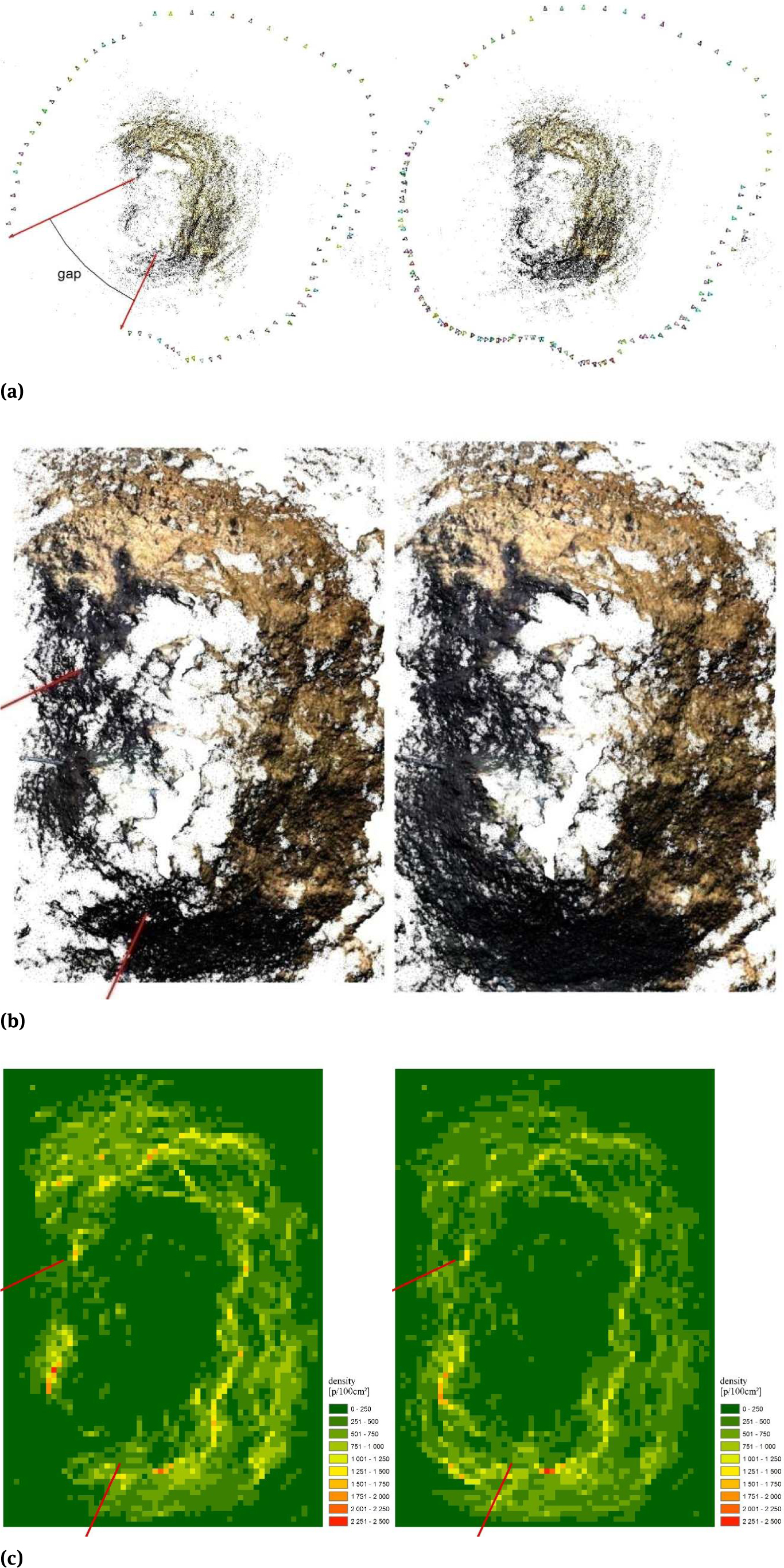
Comparison between Model 2a (left) and Model 2b (right); a) sparse model and camera position, b) dense model, c) point density in 0.1 m grid
Point density in this part of Model 2a was lower than in the corresponding part of Model 2b (Fig. 12a) in some places even by 1000 points per 100 cm2. The fact that frames were missing also influenced the values of the differences between the models calculated using CloudCompare (Fig. 12b).
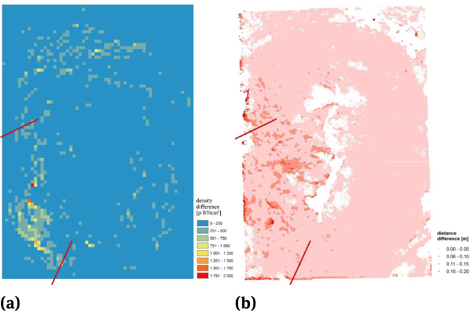
Density difference in 0.1m grid (a) and distance difference computed by CloudCompare (b)
4 Discussion
After building the model with VisualSFM it must be verified how many of the extracted frames were used. If more than 10% of the frames were rejected during model creation the reasons why it occurred and the places where it happened should be thoroughly analysed. In the situation where the model is not completed in its entirety or several successive frames are rejected in order to maintain the homogeneity of the model, the places where frames are missing can easily be identified and frame extraction frequency can be increased in them. However, this necessitates the process to be repeated and a new frame collection to be loaded to VisualSFM. Acquiring additional data can be achieved simply by extracting more frames from the video. While using still photographs, acquiring missing data require additional field measurements. It not only increases the cost of research but it can be even impossible when working with temporary objects. The research described in this article confirmed the results obtained by Gienko and Terry [43] in which it was indicated that SfM programs have a large computational power in terms of the relative orientation of images. It was also showed that they are sensitive to the number of overlapping photographs. If the convergence angles are too large the point cloud density will be visibly smaller. This relationship can be clearly observed between the marked lines in figure 9. However, the research showed that at the moment of increasing amount of images in the areas where the angle between the successive photographs was notably too large the point cloud density increased and the volume difference between models 1 and 2 decreased. The small difference between models 1 and 2b indicates that the surface of the analysed embankment is more precisely reconstructed if image density increased. Hollick et al. [50] showed that it is possible to build 3D models using sets of photograph and movie frames. However, they point out the following challenges connected with camcorder data processing: image quality (lighting, focus issues, blur and image resolution), camera calibration (unstable optics and lack of calibration), non-existent or inaccurate orientation data, large unordered dataset (heterogeneous data acquisition of the object of interest, e.g. sometimes large temporal gaps between sequences of the same object, non-optimal acquisition of data (no wide field of view or still images without sufficient overlapping areas). Additionally, the quality of frames depends on the speed of motion during recording. Hollick et al. [50], Hanif and Seghouane [51] suggest that many of the video frames in the dataset contained motion blur and proposed a method of blur removal which may be able to increase the number of key points that are able to be detected in the dataset we have used and hence improve the number of matching points between affected images. Any processing of the original image/video frame can change the number of key points. Although the authors [28] demonstrate the limitations connected with using video frames (e.g. low sharpness) the research discussed here has shown that the extracted video frames can effectively increase the density of photograph sequences used to build a model. Using videos to build a model has the advantage that, if the model fails to be created in VisualSfM, the extraction frequency can be increased without having to make another field measurement. It is possible to increase frame extraction frequency for the whole video or for selected areas, which reduces the required computational demand and reduces the calculation time. Future versions of SfM software could have modules for automatic extraction of a proper amount of frames from videos, based on quick overlap analysis.
The research has shown that although the video frames are definitely of an inferior quality than normal photographs (blurs) the models are created correctly and the possibility of extracting additional frames, an input data for model creation, proves invaluable especially in the case of temporary features, where the measurements cannot be repeated. James and Robson [52] show that SfM is a convenient technique for frequent acquisition of high-resolution 3D data, from which volumetric or crosssectional changes can be visualised and quantified. As our research has shown, when it is not necessary to provide the created models with a full georeference, their calibration can be performed using the measured distances between just two ground control points.
5 Conclusions
The videos recorded with everyday use compact cameras and smartphones can be used successfully to build DSM with SfM method.
Obtained results show great versatility of the SfM methods. It is possible to achieve reliable results using different recording devices and measurement techniques.
No significant differences between the models were found in the statistical analysis of the obtained results. This confirms that the SfM method can be used in scientific research and in engineering.
If a correct model is not built, the proposed movie-based workflow allows additional input data to be obtained by increasing the frame extraction frequency. Using a photo-based workflow would require an additional site measurement to be made, which may not be possible for temporary objects.
When building a DSM using the SfM method the quantity of and the location of the rejected photographs must be always analysed. If a model is built using a non-uniformly distributed photoset, the density of the cloud point may be non-homogenous, which affects volume calculations.
The laboratory analyses showed that using movie frames, despite their lower quality resulting for example from motion blur, models were built with volumes different from the actual volume by just 2‰ and 0.7‰.
To calculate the volume of temporary objects their models do not have to be fully georeferenced. Just two GCP pairs are sufficient. One pair used to scale the model and the second one to verify the calibration.
The advantages of the workflow proposed in the paper are the low cost resulting from the fact that technologically advanced geodesic equipment does not need to be purchased and the possibility of using free, open-source software. In comparison with geodesic methods, the proposed method reduces the time necessary to make field measurements to several minutes; however, further processing of the material obtained is more time-consuming and more complicated compared with using a dedicated commercial software.
References
[1] Westoby M.J., Brasington J., Glasser N.F., Hambrey M.J., Reynolds J.M. ‘Structure-from-Motion’ photogrammetry: A low-cost, effective tool for geoscience applications. Geomorphology 2012, 179, 300-314, DOI: 10.1016/j.geomorph.2012.08.02110.1016/j.geomorph.2012.08.021Suche in Google Scholar
[2] Singh M. K., Snehmani, Gupta R. D. Bhardwaj A, Joshi P. K., Ganju A., High resolutionDEMgeneration for complex snowcovered Indian Himalayan Region using ADS80 aerial push-broom camera: a first time attempt. Arabian Journal of Geosciences 2015, 8, 1403-1414: DOI: 10.1007/s12517-014-1299-910.1007/s12517-014-1299-9Suche in Google Scholar
[3] Roering J.J., Mackey B.H., Marshall J.A., Sweeney K.E., Deligne N.I., Booth A.M., Handwerger A.L., Cerovski-Darriau C. ‘You are HERE’: Connecting the dots with airborne lidar for geomorphic fieldwork. Geomorphology 2013, 200, 172-183, DOI: 10.1016/j.geomorph.2013.04.00910.1016/j.geomorph.2013.04.009Suche in Google Scholar
[4] Jazayeri I, Rajabifard A, Kalantari M., A geometric and semantic evaluation of 3D data sourcing methods for land and property information. Land Use Policy 2014, 36, 219-230, DOI: 10.1016/j.landusepol.2013.08.00410.1016/j.landusepol.2013.08.004Suche in Google Scholar
[5] McKean J., Roering J., Objective landslide detection and surface morphology mapping using high-resolution airborne laser altimetry. Geomorphology 2004, 57, 331-351, DOI: 10.1016/S0169-555X(03)00164-810.1016/S0169-555X(03)00164-8Suche in Google Scholar
[6] Fuller T. K., Perg L. A., Willenbring J. K., Lepper K., Field evidence for climate-driven changes in sediment supply leading to strath terrace formation. Geology 2009, 37, 467-470, DOI: 10.1130/G25487A.110.1130/G25487A.1Suche in Google Scholar
[7] Van Den Eeckhaut M., Poesen J., Gullentops F., Vandekerckhove L., Hervás J., Regional mapping and characterisation of old landslides in hilly regions using LiDAR-based imagery in Southern Flanders. Quaternary Research 2011, 75, 721-733, DOI: 10.1016/j.yqres.2011.02.00610.1016/j.yqres.2011.02.006Suche in Google Scholar
[8] Ventura G., Vilardo G., Terranova C., Sessa E. B., Tracking and evolution of complex active landslides by multitemporal airborne LiDAR data: The Montaguto landslide (Southern Italy). Remote Sensing of Environment 2011, 115, 3237-3248, DOI: 10.1016/j.res.2011.07.00710.1016/j.res.2011.07.007Suche in Google Scholar
[9] Jerolmack D. J., Ewing R. C., Falcini F., Martin R. L., Masteller C., Phillips C., Reitz M., Buynevich I. Internal boundary layer model for the evolution of desert dune fields. Nature Geoscience 2012, 5, 206–209, DOI: 10.1038/ngeo138110.1038/ngeo1381Suche in Google Scholar
[10] Brunier G., Fleury J., Anthony, E. J., Gardel A., Dussouillez P., Close-range airborne Structure-from-Motion Photogrammetry for high-resolution beach morphometric surveys: Examples from an embayed rotating beach. Geomorphology 2016, 261, 76-88, DOI: 10.1016/j.geomorph.2016.02.02510.1016/j.geomorph.2016.02.025Suche in Google Scholar
[11] Dietrich J. T., Riverscape mapping with helicopter-based Structure-from-Motion photogrammetry. Geomorphology 2016, 252, 144-157, DOI: 10.1016/j.geomorph.2015.05.00810.1016/j.geomorph.2015.05.008Suche in Google Scholar
[12] Barazzetti L., Binda L., Scaioni M., Taranto P., Photogrammetric survey of complex geometries with low-cost software: Application to the ‘G1’ temple in Myson, Vietnam. Journal of Cultural Heritage 2011, 12, 253-262, DOI: 10.1016/j.culher.2010.12.00410.1016/j.culher.2010.12.004Suche in Google Scholar
[13] DorshowW. B., Modeling agricultural potential in Chaco Canyon during the Bonito phase: a predictive geospatial approach. Journal of Archaeological Science 2012, 39, 2098-2115, DOI: 10.1016/j.jas.2012.02.00410.1016/j.jas.2012.02.004Suche in Google Scholar
[14] Hesse R., Combining Structure-from-Motion-with high and intermediate resolution satellite images to document threats to archaeological heritage in arid environments. Journal of Cultural Heritage 2016, 2, 192–201, DOI: 10.1016/j.culher.2014.04.00310.1016/j.culher.2014.04.003Suche in Google Scholar
[15] Zhang P., Arre T. J., Ide-Ektessabi A., A line scan camera-based structure from motion for high-resolution 3D reconstruction. Journal of Cultural Heritage 2016, 5, 656–663, DOI: 10.1016/j.culher.2015.01.00310.1016/j.culher.2015.01.003Suche in Google Scholar
[16] Baier W., Rando C., Developing the use of Structure-from-Motion inmass grave documentation. Forensic science international 2016, 261, 19-25, DOI: 10.1016/j.forsciint.2015.12.00810.1016/j.forsciint.2015.12.008Suche in Google Scholar PubMed
[17] Clapuyt F., Vanacker V., Van Oost K., Reproducibility of UAV-based earth topography reconstructions based on Structure-from-Motion algorithms. Geomorphology 2016, 260, 4-15, DOI: 10.1016/j.geomorph.2015.05.01110.1016/j.geomorph.2015.05.011Suche in Google Scholar
[18] Tsui O. W., Coops N. C., Wulder M. A., Marshall P. L., Integrating airborne LiDAR and space-borne radar via multivariate kriging to estimate above-ground biomass. Remote Sensing of Environment 2013, 139, 340-352, DOI: 10.1016/j.res.2013.08.01210.1016/j.res.2013.08.012Suche in Google Scholar
[19] Huang C., Peng Y., Lang M., Yeo I. Y., McCarty G., Wetland inundation mapping and change monitoring using Landsat and airborne LiDAR data. Remote Sensing of Environment 2014, 141, 231-242, DOI: 10.1016/j.res.2013.10.02010.1016/j.res.2013.10.020Suche in Google Scholar
[20] Reese H., Nyström M., Nordkvist K., Olsson H., Combining airborne laser scanning data and optical satellite data for classification of alpine vegetation. International Journal of Applied Earth Observation and Geoinformation 2014, 27, 81-90, DOI: 10.1016/j.jag.2013.05.00310.1016/j.jag.2013.05.003Suche in Google Scholar
[21] Vousdoukas M. I., Kirupakaramoorthy T., Oumeraci H., de la Torre M., Wübbold F., Wagner B., Schimmels S., The role of combined laser scanning and video techniques in monitoring wave-by-wave swash zone processes. Coastal Engineering 2014, 83, 150-165, DOI: 10.1016/j.costaleng.2013.10.01310.1016/j.costaleng.2013.10.013Suche in Google Scholar
[22] Leon J. X., Roelfsema Ch. M., Saunders M. I., Phinn S. R., Measuring coral reef terrain roughness using ‘Structure-from-Motion’ close-range photogrammetry. Geomorphology 2015, 242, 21-28, DOI: 10.1016/j.geomorph.2015.01.03010.1016/j.geomorph.2015.01.030Suche in Google Scholar
[23] Jay S., Rabatel G., Hadoux X., Moura D., Gorretta N., In-field crop row phenotyping from 3D modeling performed using Structure from Motion. Computers and Electronics in Agriculture 2015, 110, 70-77, DOI: 10.1016/j.compag.2014.09.02110.1016/j.compag.2014.09.021Suche in Google Scholar
[24] Armesto J., Roca-Pardińas J., Lorenzo H., Arias P., Modelling masonry arches shape using terrestrial laser scanning data and nonparametric methods. Engineering Structures 2010, 32, 607-615, DOI: 10.1016/j.engstruct.2009.11.00710.1016/j.engstruct.2009.11.007Suche in Google Scholar
[25] Bhatla A., Choe S. Y., Fierro O., Leite F., Evaluation of accuracy of as-built 3D modeling from photos taken by handheld digital camera. Automation in Construction 2012, 28, 116–127, DOI: 10.1016/j.autcon.2012.06.00310.1016/j.autcon.2012.06.003Suche in Google Scholar
[26] González-Jorge H., Riveiro B., Arias P., Armesto J., Photogrammetry and laser scanner technology applied to length measurements in car testing laboratories. Measurement 2012, 45, 354-363, DOI: 10.1016/j.measurement.2011.11.01010.1016/j.measurement.2011.11.010Suche in Google Scholar
[27] Remondino F., El-Hakim S., Image-based 3D modeling: a review. The Photogrammetric Record 2006, 21, 269–291, DOI: 10.1111/j.1477-9730.2006.00383.x10.1111/j.1477-9730.2006.00383.xSuche in Google Scholar
[28] Alsadik B., Remondino F., Menna F., Gerke M., Vosselman G., Robust extraction of image correspondences exploiting the image scene geometry and approximate camera orientation. 3D-ARCH 2013 - 3D Virtual Reconstruction and Visualization of Complex Architectures, 2013, Trento, Italy. International Archives of the Photogrammetry, Remote Sensing and Spatial Information Sciences. XL-5/W110.5194/isprsarchives-XL-5-W1-1-2013Suche in Google Scholar
[29] Bryson M., Johnson-Roberson M., Murphy R., Bongiorno J., Kite aerial photography for low-cost, ultra-high spatial resolution multi-spectral mapping of intertidal landscapes. PLoS ONE 2013, 8(9), DOI: 10.1371/journal.pone.007355010.1371/journal.pone.0073550Suche in Google Scholar PubMed PubMed Central
[30] Gomez Ch., Hayakawa Y., Obanawa H., A study of Japanese landscapes using structure from motion derived DSMs and DEMs based on historical aerial photographs: New opportunities for vegetation monitoring and diachronic geomorphology. Geomorphology 2015, 242, 11-20, DOI: 10.1016/j.geomorph.2015.02.02110.1016/j.geomorph.2015.02.021Suche in Google Scholar
[31] Anderson K., Griflths D., DeBell L., Hancock S., Duffy J.P., Shutler J.D., Reinhardt J., A. Griflths A., A Grassroots Remote Sensing Toolkit Using Live Coding, Smartphones, Kites and Lightweight Drones. PLoS ONE 2016, 11(5), DOI: 10.1371/journal.pone.015156410.1371/journal.pone.0151564Suche in Google Scholar PubMed PubMed Central
[32] Niethammer U., James M. R., Rothmund S., Travelletti J., Joswig M., UAV-based remote sensing of the Super-Sauze landslide: Evaluation and results. Engineering Geology 2012, 128, 2-11, DOI: 10.1016/j.enggeo.2011.03.01210.1016/j.enggeo.2011.03.012Suche in Google Scholar
[33] Dandois J. P., Ellis E.C., High spatial resolution Three-dimensional mapping of vegetation spectral dynamics using computer vision. Remote Sensing of Environment 2013, 136, 259–276, DOI: 10.1016/j.rse.2013.04.00510.1016/j.rse.2013.04.005Suche in Google Scholar
[34] Lucieer A., Turner D., King D. H., Robinson S. A., Using an Unmanned Aerial Vehicle (UAV) to capture micro-topography of Antarctic moss beds. International Journal of Applied Earth Observation and Geoinformation 2013, 27, 53-62, DOI: 10.1016/j.jag.2013.05.01110.1016/j.jag.2013.05.011Suche in Google Scholar
[35] Snavely K.N. Scene reconstruction and visualization from Internet photo collections. PhD thesis, University of Washington, USA, 2008Suche in Google Scholar
[36] Tonkin T. N., Midgley N. G., Graham D. J., Labadz J. C., The potential of small unmanned aircraft systems and structure-from-motion for topographic surveys: A test of emerging integrated approaches at Cwm Idwal, North Wales. Geomorphology 2014, 226, 35-43, DOI: 10.1016/j.geomorph.2014.07.02110.1016/j.geomorph.2014.07.021Suche in Google Scholar
[37] Wu C., Towards Linear-time Incremental Structure from Motion. IEEE 2013. International Conference on 3D Vision, 2012, Seattle, WA, USA, 127-134, DOI: 10.1109/3DV.2013.2510.1109/3DV.2013.25Suche in Google Scholar
[38] Szeliski R., Kang S. B., Recovering 3D shape and motion from image streams using nonlinear least squares. Journal of Visual Communication and Image Representation 1994, 5, 10-28, DOI: 10.1006/jvci.1994.100210.1006/jvci.1994.1002Suche in Google Scholar
[39] Wu C., Agarwal S., Curless B., Seitz S. M., Multicore Bundle Adjustment. In: IEEE conference on Computer Vision and Pattern Recognition (CVPR), Colorado Springs, USA, 3057 – 3064, DOI: 10.1109/CVPR.2011.599555210.1109/CVPR.2011.5995552Suche in Google Scholar
[40] Tarolli P., High-resolution topography for understanding Earth surface processes: Opportunities and challenges. Geomorphology 2014, 216, 295-312, DOI: 10.1016/j.geomorph.2014.03.00810.1016/j.geomorph.2014.03.008Suche in Google Scholar
[41] Fonstad M. A., Dietrich J. T., Courville B. C., Jensen J. L., Carbonneau P. E., Topographic structure from motion: a new development in photogrammetric measurement. Earth surface processes and Landforms 2013, 38, 421-430, DOI: 10.1002/esp.336610.1002/esp.3366Suche in Google Scholar
[42] Carrivick J. L., Geilhausen M., Warburton J., Dickson N. E., Carver S. J., Evans A.J., Brown L.E., Contemporary geomorphological activity throughout the proglacial area of an alpine catchment. Geomorphology 2013, 188, 83-95, DOI: 10.1016/j.geomorph.2012.03.02910.1016/j.geomorph.2012.03.029Suche in Google Scholar
[43] Gienko G.A., Terry J.P., Three-dimensional modeling of coastal boulders using multi-view image measurements. Earth surface processes and Landforms 2013, 39, 853-864, DOI: 10.1002/esp.348510.1002/esp.3485Suche in Google Scholar
[44] Javernick L., Brasington J., Caruso B., Modeling the topography of shallow braided rivers using Structure-from-Motion photogrammetry. Geomorphology 2014, 213, 166-182, DOI: 10.1016/j.geomorph.2014.01.00610.1016/j.geomorph.2014.01.006Suche in Google Scholar
[45] Golparvar-Fard M., Bohn J., Teizer J., Savarese S., Peńa-Mora F., Evaluation of image-based modeling and laser scanning accuracy for emerging automated performance monitoring techniques. Automation in Construction 2011, 20, 1143–1155, DOI: 10.1016/j.autcon.2011.04.01610.1016/j.autcon.2011.04.016Suche in Google Scholar
[46] Jancosek M, Pajdla T. Multi-view reconstruction preserving weakly-supported surfaces. In: IEEE conference on Computer Vision and Pattern Recognition (CVPR), Colorado Springs, USA, 2011, 3121 – 3128, DOI: 10.1109/CVPR.2011.599569310.1109/CVPR.2011.5995693Suche in Google Scholar
[47] Cignoni P., Corsini M., Ranzuglia G., Meshlab: an open-source 3d mesh processing system, ERCIM News, 73, 2008, 45-46Suche in Google Scholar
[48] Girardeau-Montaut D. et al. CloudCompere User’s Manual for version 2.1, 2012Suche in Google Scholar
[49] Aspert N., Santa Cruz D., Ebrahimi T., MESH: measuring errors between surfaces using the Hausdorff distance. In Proc of the IEEE International Conference in Multimedia and Expo 2002, Lausanne, Switzerland, 1, 705-708, DOI: 10.1109/ICME.2002.103587910.1109/ICME.2002.1035879Suche in Google Scholar
[50] Hollick J., Moncrieff S., Belton D., Woods A.J., Hutchison A., Helmholz P., Creation of 3d models from large unstructured image and video datasets. ISPRS Hannover Workshop, 2013, Hannover, Germany. International Archives of the Photogrammetry, Remote Sensing and Spatial Information Sciences, Volume XL-1/W110.5194/isprsarchives-XL-1-W1-133-2013Suche in Google Scholar
[51] Hanif M., Seghouane A., Blurred Image Deconvolution Using Gaussian Scale Mixtures Model in Wavelet Domain. IEEE 2012 International Conference on Digital Image Computing Techniques and Applications, 2012, 1-6, DOI: 10.1109/DICTA.2012.641169210.1109/DICTA.2012.6411692Suche in Google Scholar
[52] James M.R., Robson S., Straightforward reconstruction of 3D surfaces and topography with a camera: Accuracy and geoscience application. Journal of Geophysical Research, 117, 2012, 2156-2202, DOI: 10.1029/2011JF00228910.1029/2011JF002289Suche in Google Scholar
© 2017 Rafał Wróżyński et al.
This work is licensed under the Creative Commons Attribution-NonCommercial-NoDerivatives 3.0 License.
Artikel in diesem Heft
- Regular Articles
- Two types of gabbroic xenoliths from rhyolite dominated Niijima volcano, northern part of Izu-Bonin arc: petrological and geochemical constraints
- Regular Articles
- CRSP, numerical results for an electrical resistivity array to detect underground cavities
- Regular Articles
- Magma evolution inside the 1631 Vesuvius magma chamber and eruption triggering
- Regular Articles
- Probabilities of Earthquake Occurrences along the Sumatra-Andaman Subduction Zone
- Regular Articles
- Modelling of carrying capacity in National Park - Fruška Gora (Serbia) case study
- Regular Articles
- Knickzone Extraction Tool (KET) – A new ArcGIS toolset for automatic extraction of knickzones from a DEM based on multi-scale stream gradients
- Regular Articles
- When the display matters: A multifaceted perspective on 3D geovisualizations
- Regular Articles
- Dependence of Gully Networks on Faults and Lineaments Networks, Case Study from Hronska Pahorkatina Hill Land
- Regular Articles
- Environmental Geochemistry of Geophagic Materials from Free State Province in South Africa
- Regular Articles
- Neotectonic interpretations and PS-InSAR monitoring of crustal deformations in the Fujian area of China
- Regular Articles
- Dual-shale-content method for total organic carbon content evaluation from wireline logs in organic shale
- Regular Articles
- The dolerite dyke swarm of Mongo, Guéra Massif (Chad, Central Africa): Geological setting, petrography and geochemistry
- Regular Articles
- Seismic data filtering using non-local means algorithm based on structure tensor
- Regular Articles
- Pore Distribution Characteristics of the Igneous Reservoirs in the Eastern Sag of the Liaohe Depression
- Regular Articles
- Three-dimensional structural model of the Qaidam basin: Implications for crustal shortening and growth of the northeast Tibet
- Regular Articles
- Failure Mode of the Water-filled Fractures under Hydraulic Pressure in Karst Tunnels
- Regular Articles
- Creating a low carbon tourism community by public cognition, intention and behaviour change analysisa case study of a heritage site (Tianshan Tianchi, China)
- Regular Articles
- Mapping Mangrove Density from Rapideye Data in Central America
- Regular Articles
- Marine sediment cores database for the Mediterranean Basin: a tool for past climatic and environmental studies
- Regular Articles
- Retrofitting the Low Impact Development Practices into Developed Urban areas Including Barriers and Potential Solution
- Regular Articles
- Spatial uncertainty of a geoid undulation model in Guayaquil, Ecuador
- Regular Articles
- Structure and Filling Characteristics of Paleokarst Reservoirs in the Northern Tarim Basin, Revealed by Outcrop, Core and Borehole Images
- Regular Articles
- Ground volume assessment using ’Structure from Motion’ photogrammetry with a smartphone and a compact camera
- Regular Articles
- Classification of coal seam outburst hazards and evaluation of the importance of influencing factors
- Regular Articles
- Geochemical characterization of Neogene sediments from onshore West Baram Delta Province, Sarawak: paleoenvironment, source input and thermal maturity
- Regular Articles
- Influence of Social-economic Activities on Air Pollutants in Beijing, China
- Regular Articles
- Spectral properties of weathered and fresh rock surfaces in the Xiemisitai metallogenic belt, NW Xinjiang, China
- Regular Articles
- Geochemistry of sandstones and shales from the Ecca Group, Karoo Supergroup, in the Eastern Cape Province of South Africa: Implications for provenance, weathering and tectonic setting
- Regular Articles
- Petrology and geochemistry of meta-ultramafic rocks in the Paleozoic Granjeno Schist, northeastern Mexico: Remnants of Pangaea ocean floor
- Regular Articles
- Distal turbidite fan/lobe succession of the Late Oligocene Zuberec Fm. – architecture and hierarchy (Central Western Carpathians, Orava–Podhale basin)
- Regular Articles
- Fourier Transform Infrared Spectroscopy of Clay Size Fraction of Cretaceous-Tertiary Kaolins in the Douala Sub-Basin, Cameroon
- Regular Articles
- Optimized AVHRR land surface temperature downscaling method for local scale observations: case study for the coastal area of the Gulf of Gdańsk
- Regular Articles
- New non-linear model of groundwater recharge: Inclusion of memory, heterogeneity and visco-elasticity
- Regular Articles
- “Urban geosites” as an alternative geotourism destination - evidence from Belgrade
- Regular Articles
- A customized resistivity system for monitoring saturation and seepage in earthen levees: installation and validation
- Regular Articles
- Consideration of Landsat-8 Spectral Band Combination in Typical Mediterranean Forest Classification in Halkidiki, Greece
- Regular Articles
- Coda Wave Attenuation Characteristics for North Anatolian Fault Zone, Turkey
- Regular Articles
- Modal composition and tectonic provenance of the sandstones of Ecca Group, Karoo Supergroup in the Eastern Cape Province, South Africa
- Regular Articles
- Quantitative studies of the morphology of the south Poland using Relief Index (RI)
- Regular Articles
- Interpretation of sedimentological processes of coarse-grained deposits applying a novel combined cluster and discriminant analysis
- Regular Articles
- Utilizing borehole electrical images to interpret lithofacies of fan-delta: A case study of Lower Triassic Baikouquan Formation in Mahu Depression, Junggar Basin, China
- Regular Articles
- Grain size statistics and depositional pattern of the Ecca Group sandstones, Karoo Supergroup in the Eastern Cape Province, South Africa
- Regular Articles
- Carbonate stable isotope constraints on sources of arsenic contamination in Neogene tufas and travertines of Attica, Greece
- Regular Articles
- Appreciation of landscape aesthetic values in Slovakia assessed by social media photographs
- Regular Articles
- Geochemistry of Selected Kaolins from Cameroon and Nigeria
- Regular Articles
- Spatial pattern of ASG-EUPOS sites
- Regular Articles
- A Stream Tilling Approach to Surface Area Estimation for Large Scale Spatial Data in a Shared Memory System
- Regular Articles
- A location-based multiple point statistics method: modelling the reservoir with non-stationary characteristics
- Regular Articles
- Water Inrush Analysis of the Longmen Mountain Tunnel Based on a 3D Simulation of the Discrete Fracture Network
- Regular Articles
- A Computer Program for Practical Semivariogram Modeling and Ordinary Kriging: A Case Study of Porosity Distribution in an Oil Field
- Regular Articles
- Imaging and locating paleo-channels using geophysical data from meandering system of the Mun River, Khorat Plateau, Northeastern Thailand
- Regular Articles
- Rare earth element contents of the Lusi mud: An attempt to identify the environmental origin of the hot mudflow in East Java – Indonesia
- Regular Articles
- Is Nigeria losing its natural vegetation and landscape? Assessing the landuse-landcover change trajectories and effects in Onitsha using remote sensing and GIS
- Regular Articles
- Methodological approach for the estimation of a new velocity model for continental Ecuador