Knickzone Extraction Tool (KET) – A new ArcGIS toolset for automatic extraction of knickzones from a DEM based on multi-scale stream gradients
-
Tuba Zahra
 ,
Uttam Paudel
,
Uttam Paudel

Abstract
Extraction of knickpoints or knickzones from a Digital Elevation Model (DEM) has gained immense significance owing to the increasing implications of knickzones on landform development. However, existing methods for knickzone extraction tend to be subjective or require time-intensive data processing. This paper describes the proposed Knickzone Extraction Tool (KET), a new raster-based Python script deployed in the form of an ArcGIS toolset that automates the process of knickzone extraction and is both fast and more user-friendly. The KET is based on multi-scale analysis of slope gradients along a river course, where any locally steep segment (knickzone) can be extracted as an anomalously high local gradient. We also conducted a comparative analysis of the KET and other contemporary knickzone identification techniques. The relationship between knickzone distribution and its morphometric characteristics are also examined through a case study of a mountainous watershed in Japan.
1 Introduction
A knickzone is a locally steep segment along the longitudinal profile of a river, depending on its length often referred to as a knickpoint, considering that the length is short and regarded as a point on the longitudinal profile [1–4]. Knickzones in the form of waterfalls often occur in bedrock rivers [5–7] and are an indicator of channel adjustments to local or regional perturbations [8–10]. The steepening of a river reach occurs as a result of a number of factors and processes including resistant lithology and differential erosion [2, 11, 12], transient response to base level change [13, 14], change in shear stress leading to gully head propagation [15], and changes in sediment loads from tributaries [16]. Knickzones that develop along the stream thalwegs or bedrocks influence the shape and trend of the longitudinal channel profiles. The controls of bedrock geology such as lithology, stratigraphy and structure on knickzone origin, morphology and evolution is a key component in geomorphic research [17].
Morphometric analysis of longitudinal profiles with a knickpoint or knickzone has been used to understand landscape evolution with respect to local anomalies in tectonics and lithology, hydraulics, associated base-level changes, deformation of valley-side slopes and landslide damming, as well as sediment size [e.g. 18–20]. In spite of the widening scope of research in knickzone modeling [21], generating a regional scale map of knickzones remains a challenge. Regional knickzone distribution maps are not only valuable resources for fluvial geomorphology [18, 22] but are recently being incorporated into mass-wasting inventories for improved detection of debris flow [20].
Traditionally, knickzones are identified by visual inspection of river longitudinal profiles or their slope-area relationships [23–25]. Such manual interpretations make the studies subjective. Field observations and surveys for morphologically identifying knickzones [26–28] are also tedious. Therefore, some studies have pursued automated approaches for knickzone extraction. For example, Whipple et al. [29] applied the Stream Profiler Tool (SPT), and Hill and Stewart [30] used local changes in the normalized steepness index (ksn) from upstream to downstream.
Another method of knickzone extraction based on changes in stream gradient with respect to spatial scale was proposed by Hayakawa and Oguchi [3] that used a DEM (Digital Elevation Model) and GIS (Geographical Information System). The method consisted of a vector-based semi-automated procedure that required somewhat time-intensive data processing (c.f. Section 3.3.1 for the processing time taken for each method) because of the independent use of GIS and spreadsheet software. Several studies, however, have applied their approach and found it to be useful [4, 31–33].
To expedite the knickzone identification process, we developed a new raster-based software program called the Knickzone Extraction Tool (KET). Programmed in Python and deployed as an ArcGIS toolset, this tool automates the entire process, making the extraction of knickzones faster and more user-friendly. We also conducted a case study in a mountainous area of central Japan to evaluate the performance of the KET and investigate the relationship between knickzone properties and environmental factors.
2 Methods of automated knickzone extraction
This section briefly explains the existing tools or methods for knickzone extraction and comprises of two parts, Section 2.1 and 2.2. The former explains the existing methods of knickzone extraction that are popularly used and/or are in use, while the later introduces the Knickzone Extraction Tool (KET).
2.1 Existing methods
The existing methods include: the SPT [29, 43] the GIS-Knickfinder [34], and the semi-automatic extraction method of Hayakawa and Oguchi ([3]; hereafter referred to as SAKE). They are based on three distinct geomorphic properties: slope-area, slope-curvature, and stream gradient, respectively.
2.1.1 Stream Profiler Tool (SPT)
Based on the slope-area approach, the SPT uses ArcGIS (9x and 10x) and MATLAB (R2012a and later versions) to analyze the steepness index and concavity of river profiles [29]. The knickzones are thereby determined from an evaluation of the steepness index. The basic equation underlying the tool is:
This relationship is known as the Flint’s Law [35] where S is the local channel slope, A the upstream drainage area, ksthe steepness index, and θ is the dimensionless concavity index of the curve. ks is used to identify knickzones as anomalies (deviations) from the trend of the river longitudinal profile. Although the SPT is widely applied to study the effects of tectonics, it is time intensive. The SPT uses the built-in hydrology and surface tools of ArcGIS (9x and 10x) for extracting the drainage components of flow direction, flow accumulation, catchment area, and other attributes such as channel slope, followed by visually interpreting plots of channel parameters to demarcate knickzones.
2.1.2 GIS-Knickfinder (GKF)
Based on ArcGIS (10x) and Python libraries, the GKF uses the slope-curvature approach applied to the entire raster layer instead of analyzing stream profiles individually [34]. The tool contains a set of algorithms related to drainage area and plan curvature. Knickzones (referred to as headcuts in the tool) are identified as pixels with a curvature less than a certain threshold and a drainage area greater than a certain threshold.
The curvature threshold is the key to identifying knickzones based on terrain shape, whereas the drainage area threshold is used to exclude knickzones that are not along the main channel. The curvature values for a hilly area with moderate relief vary between −0.5 and 0.5, whereas for steep, rugged mountains (extreme relief), the values vary between −4 and 4 ([7]; Francis Rengers, personal communication). Curvature values may exceed these ranges for different areas depending on the topographical characteristics. The knickzones for each bedrock river can then be extracted by overlaying the vector line data showing the distribution of bedrock rivers.
2.1.3 Semi-Automatic Extraction (SAKE) Method
The SAKE method [3] is based on the assumption that the slope gradient along a river changes with measurement length, and a locally steep segment of the riverbed is considered a knickzone. The gradient of a river reach is:
where e1 is the riverbed elevation d/2 upstream of a measuring point along a stream, e2 is the riverbed elevation d/2 downstream, Gd (m m−1) is the stream gradient at the measuring point, and d (m) is the variable measurement distance (Fig. 1a). SAKE calculates the scale-dependent change in Gd (m m−1) by solving a linear regression equation:

Illustrated explanation highlighting the difference between SAKE and KET methods. SAKE considers both the upstream (e1) and the downstream (e2) elevations that are d/2 apart, whereas KET uses the elevation at the point e0 and d downstream at point e3
where d is the multi-scale measurement length, a is the regression coefficient, and b is the intercept.
The relative steepness index Rd is then defined as:
which represents the rate of gradient decrease with increasing d. Rd shows how steep the point is locally compared to the trend of the stream gradient averaged over a longer d, and a threshold of Rd can be defined for identification of knickzones. An average of the standard deviations of Rd for all the rivers in a region is then used as the threshold [3].
SAKE has been applied for a regional scale analysis, and it has also been used to provide data on knickzone properties such as height, length, and gradient. These properties have been studied in relation to the altitude, upstream distance, drainage area, and geology to understand factors controlling knickzone formation [3, 33, 36, 37]. However, wider application of SAKE requires technical improvement, because it requires time-intensive data processing resulting from the separate use of ArcGIS (10x) and spreadsheet software.
2.2 New method: Knickzone Extraction Tool (KET)
The KET, a new raster-based Python script deployed in the form of an ArcGIS toolset, is proposed in this study. The KET intends to automate the process of SAKE for faster and more user-friendly knickzone extraction, but there are some differences from SAKE for technical reasons. For example, KET calculates Gd using the following equation:
SAKE considers both the upstream and downstream elevations d/2 apart (Figure 1a, Equation 2), whereas KET uses the elevation at the point e0 and d downstream at point e3 (Figure 1b). The method of SAKE considers both the upstream and downstream elevations for detecting a locally steep segment; this method, however, is inapplicable to the uppermost section of the river. KET is applicable from the top of the river, so it requires a simple algorithm that follows the flow direction and is free from the ambiguity of determining the uppermost point of the river. This program, available as an ArcGIS toolset, utilizes the built-in spatial analyst functions in ArcGIS [38] for creating a hydrologically corrected (sink-filled) DEM and extracting the flow direction. Terrain analysis using DEM (TauDEM; [39]), is used for computing slope averaged over a selected distance (SLPD) along the direction of flow. Figure 2 shows the flow chart of the KET algorithm that calculates SLPD for different d values from dmin to dmax (the range of the gradient analysis) and represents the data as raster layers. The SLPD raster layers are used in the following equation for the calculation of Rd as a negative product of the regression coefficient signifying the decrease in gradient.

Flow chart of the algorithm used for Knickzone Extraction Tool (KET). The mathematical expression of Rd is explained in Equation 6.
where n = (dmax − dmin) / f (d), xi = i × f (d) n, SLPDi is the i-th SLPD with f (d) being a function of d that expresses the change in the multi-scale measurement distance from xi to xi+1. While Equation 4 provides numerical values of Rd for the downstream river gradient over a larger distance using elevation values, Equation 6 represents this value by averaging slope over marginal distances, resulting in raster layers. This raster-based approach that provides a regional raster layer of Rd values is advantageous compared to the manual calculation of Rd within individual river profiles. Using a threshold of Rd for extracting knickzones, KET identifies knickzones along with their height, length, distance from the stream top, and distance from the river mouth like SAKE.
3 Case study
This section comprises of three subsections that include a description of the study area (Section 3.1), the applications of the new and existing methods of knickzone extraction with parameter values for the study area (Section 3.2), and the results of comparison of these methods (Section 3.3). We demonstrate this case study for a mountainous watershed with diverse topographic and geologic conditions in central Japan, providing an opportunity to assess the validity of the knickzone extraction methods with certain parameters.
3.1 Study area and data used
The study area (Figure 3) is a mountainous region of the southwestern side of the Northern Japanese Alps, Gifu Pre fecture, Japan. The study area consists of regular volcanic, plutonic and accretionary rocks in a region of varying topographies [40, 41]. The precipitation data from the nearest station (Takayama City; Japan Meteorological Agency) shows that the region receives average annual rainfall of 1700 mm (1981–2010). A number of waterfalls such as the Neo-no-taki Falls and the Mitsudaki Falls exist within the watershed that are less accessible and are limited to direct anthropogenic effects. Therefore, the watershed seems to be suitable for knickzone analysis.

Case study area; Inset - map of Japan with the Gifu Prefecture and the study area.
We used a 10-m DEM from the Hokkaido Chizu Corporation, Asahikawa, Japan with a UTM Projection (zone 53N) and a vector map of all the bedrock rivers in Japan (National Institute of Industrial Science and Technology, 2012). As measured from the later, the total length of the bedrock rivers studied was 742 km. A digital vector map of dam locations in Japan (National Land Numerical Information, 2009) was also used to avoid misidentification of dams as knickzones. In addition, a database of knickzone distribution based on a 50-m DEM [3, 4] was also used to extract knickzones inthe study area.
3.2 Application of the knickzone extraction methods
The four knickzone extraction methods described in Section 2 were applied to the case study area to obtain knickzone distribution maps. Knickzones with a length > 30 m and height ≥ 15 m were identified as well-defined knickzones. The range of stream length for gradient analysis using SAKE and KET (dmin to dmax) is 30 to 1500 m based on the spatial resolution of the DEM and varies with a step of 30 m. The height threshold of ≥ 15 m reflects the vertical accuracy of the DEM (originally prepared using topo-map contours with 10 m intervals) and the existence of small check dams that are not included in the dam data.
To extract knickzones with the SPT method, a concavity index (θ) for all the bedrock reaches is required (Equation 1). The calculated concavity index of 0.5 is used. Similarly, for GKF a mean curvature value is required and was calculated to be −0.49. A curvature threshold of −4 was used for this study because a threshold of −5 led to under-extraction of knickzones. Since the area has varying topography the value of channel curvature (θ) of the longitudinal profile from the head to the watershed outlet is the same for the entire length of the channel. But difference in gradient produces very different channel forms that influence the local curvatures values. Underestimates of knickzones might occur because the same curvature values (here −5) can exist for bedrock rivers having different gradients. The trend gradient threshold used for the SAKE method is 1.92 × 10⁻⁴ m−1, based on the sum of mean and standard deviation of Rd for all the bedrock reaches in the study area, following the guideline of Hayakawa and Oguchi [3]. This threshold was also applied for extracting well-defined knickzones using KET (hereafter referred to as KET2), thereby reducing the number of ambiguous knickzones. For comparison, the threshold value 1.42 × 10⁻⁵ m−1 from Hayakawa and Oguchi [4] was also used (hereafter known as KET1).
The general properties of knickzones, such as their frequency (the total number of knickzones divided by the total length of bedrock reaches), density (the total length of knickzones divided by the total length of bedrock reaches), and forms including the average height, length and gradient (height divided by length) were calculated for knickzones using the four methods. Although the original version of the GKF only provides concavity values of knickzones, we also extracted the height, length, and gradient properties.
Note that knickpoints from SPT are point data (knickpoints) along the river profile. As such, knickzone form characteristics like height, length, and gradient are not available. Characteristics like distance of the knickpoints from the river head and the watershed outlet were calculated from vector data of bedrock rivers because SPT does not provide them automatically. Alternatively, ks (from SPT) indicates the scaling between drainage area and channel slope and the parameters of the Flint’s Law (Equation 1) morphological characteristics of the river profiles. Similarly, morphological indices like mean concavity (from GKF) and Rd values (from SAKE and KET) were obtained for each knickzone.
Furthermore, we analyzed the locational intersection between knickzones based on whether a knickzone identified using one method exists within a certain distance of one identified using another method. In other words, an analysis of the intersection of knickzones within a certain distance is conducted. For the intersection distance, six values are used: 15, 30, 45, 60, 75, and 90 m. This analysis gives information about over- and under-extraction of knickzones using a certain method.
The results from the four methods using a 10-m DEM are also compared with the knickzones identified by Hayakawa and Oguchi [4] who used the SAKE method and a 50-m DEM. SAKE using a 10-m DEM is hereafter referred to as SAKE10, and SAKE using the 50-m DEM is referred to as SAKE50. It should be noted that SAKE50 is also used for the validation of knickzones since field validation of knickzones was difficult and SAKE50 includes some validated knickpoints from previous studies [42]. Additionally, the KET was run on the 50-m DEM (hereafter KET50) with the same threshold value as in Hayakawa and Oguchi [4] to test the influence of grid resolution on the distribution of knickzones. Trial runs were conducted with SAKE and KET (using a 64-bit operating system with a processing speed of 3.40 GHz and a 16 Gb RAM) to compare the time required for extracting knickzones using each method.
In addition, the frequency of knickzones was also computed for each bin of locational factors such as altitude, distance from watershed outlet, drainage area and the stream gradient for d = 750 m. This value of d was selected based on a gradient analysis conducted using the SAKE method, where the stream length gradient of all streams indicated changes at d = 750 m, thus demarcating it as the trend gradient for streams in the study area.
3.3 Results
This section comprises of results from the comparative analyses of the new and existing methods of knickzone extraction, and has been grouped into three subsections: the spatial distribution of the knickzones extracted (Section 3.3.1), their intersections (Section 3.3.2), and their properties and morphometric characteristics (Section 3.3.3).
3.3.1 Distribution and basic properties of knickzones
Distribution maps of the knickzones extracted based on the aforementioned methods depict high knickzone concentrations in the mountainous areas and southwestern slopes of Mount Ontake (Figure 4). The spatial distribution of knickzones in the study area determine their locational properties and the morphometric characteristics of knickzones and have been discussed briefly in Section 3.3.3.

Distribution maps of knickzones extracted using the methods in Section 2: a. STP; b. GKF; c. SAKE10; d. SAKE50; e. KET1; f. KET2, and g. KET50 (c.f. Section 3.2)
Using SPT, a total of 113 knickzones were extracted (Figure 4a). The frequency of the knickzones was 0.15 km−1, with a mean upstream drainage area of 284.49 km2 and a mean ks of 148.57. Individual extraction of 15 bedrock river longitudinal profiles and their knickzone extraction using the interactive profile and slope-area graphs in MATLAB and ArcGIS requires approximately one day. This time requirement, however, is dependent on the study area and the number of longitudinal profiles observed.
With the GKF tool, a total of 16 knickzones were extracted (Figure 4b). The mean concavity of all the bedrock streams was −0.49. The frequency of the knickzones was 0.02 km−1, with a mean concavity of −7.93 indicating a high overall concavity. The percentage of knickzones in terms of length, in other words, density of knickzones was very low (0.33%). The time required to run the GKF tool on a 10-m DEM was approximately one day.
SAKE10 resulted in 141 knickzones (Figure 4c) with a frequency of 0.2 km−1. The density of knickzones was 1.3%. The mean height of the knickzones was 27.47 m, the mean length was 69.68 m, the average gradient was 0.38 m m−1, and the mean relative steepness index (Rd) was 5.8 × 10⁻³ m−1. SAKE50 extracted 58 knickzones (Figure 4d) for the study area with a frequency of 0.08 km−1. The density of knickzones was 2.4% while the mean height, length, and gradient were 68.51 m, 311.72 m, and 1.73 m m−1, respectively. The mean Rd was 3.58 × 10⁻⁵ m−1. SAKE took less than 2 h to calculate Rd values for each longitudinal profile, but extracting the knickzones and their properties using spreadsheets took more than one day.
KET1 resulted in a total of 189 knickzones (Figure 4e). The knickzone frequency is 0.25 km−1. The density of knickzones was very high (8.14%) because each knickzone was long. The mean height, length, and gradient of the knickzones were 33.83 m, 319.68 m, and 0.14 m m−1 respectively. The average relative steepness was −0.68 × 10⁻⁴ m−1. KET2 extracted 20 knickzones (Figure 4f). The knickzone frequency was 0.02 km−1 and the knickzone density was 0.32%. The mean value of knickzone length, height, and gradient were 48.43 m, 120 m, and 0.47 m m−1 respectively. The average relative steepness was −2.71 × 10⁻⁴ m−1. KET50 resulted in 111 knickzones (Figure 4g), with the knickzone frequency of 0.15 km−1. The knickzone density is high (7.5%). The mean height, length, and gradient of the knickzones were 97.92 m, 501.22 m, and 0.16 m m−1, respectively. The average relative steepness was −2.78 × 10⁻⁵ m−1. The average time required for trial runs of KET using a 50-m DEM in the study area was 15-20 minutes, while that for a 10-m DEM was 45-50 minutes. For comparison, the basic statistical values from the four methods with the results from different grid resolution DEMs and SAKE50 are shown in Table 1.
General statistical properties of knickzone forms
| Statistics of form properties | ||||||
|---|---|---|---|---|---|---|
| Methods | Properties | Units | Mean | Standard Deviation | Minimum | Maximum |
| GKF | Height | m | 31.37 | 20.49 | 16.36 | 96.85 |
| Length | m | 81.62 | 53.68 | 22.60 | 200.36 | |
| Gradient | m m−1 | 0.50 | 0.30 | 0.10 | 1.28 | |
| Concavity | −7.93 | 1.44 | −10.71 | −5.99 | ||
| SAKE10 | Height | m | 27.47 | 13.92 | 15.05 | 89.12 |
| Length | m | 69.68 | 19.52 | 45.00 | 165.00 | |
| Gradient | m m−1 | 0.38 | 0.15 | 0.14 | 0.99 | |
| Mean Rd | ×10−3 m−1 | 0.58 | 0.26 | 0.24 | 2.21 | |
| KET1 | Height | m | 33.83 | 20.73 | 15.00 | 97.00 |
| Length | m | 319.68 | 258.16 | 50.00 | 1770.00 | |
| Gradient | m m−1 | 0.14 | 0.08 | 0.02 | 0.5 | |
| Mean Rd | ×10−4 m−1 | −0.68 | 0.30 | −1.97 | −0.25 | |
| KET2 | Height | m | 48.43 | 21.94 | 20.13 | 106.51 |
| Length | m | 120 | 59.03 | 40 | 240 | |
| Gradient | m m−1 | 0.47 | 0.26 | 0.2 | 1.15 | |
| Mean Rd | ×10−4 m−1 | −2.71 | 5.82 | −4.28 | −2.02 | |
| KET50 | Height | m | 97.92 | 130.43 | 5.54 | 952.56 |
| Length | m | 501.22 | 450.69 | 60 | 2985 | |
| Gradient | m m−1 | 0.16 | 0.08 | 0.03 | 0.36 | |
| Mean Rd | ×10−5 m−1 | −2.78 | 0.96 | −6.22 | −1.65 | |
| SAKE50 | Height | m | 68.51 | 64.61 | 11.10 | 355.10 |
| Length | m | 311.72 | 137.91 | 160.00 | 880.00 | |
| Gradient | m m−1 | 1.73 | 1.29 | 0.92 | 7.86 | |
| Mean Rd | ×10−5 m−1 | 3.58 | 2.00 | 1.63 | 10.81 | |
NOTE: Knickpoints from STP are point data only, therefore form properties are not available.
3.3.2 Intersection of knickzones
Regarding the intersection of knickzones (Table 2), 36.28% of knickzones from KET1 were found within 90 m of knickzones extracted using the SAKE10 method. Interestingly, 76.25% of knickzones from SAKE10 were within 90 m of SPT knickzones, which was closely followed by 74.65% within 90 m of GKF knickzones; 59.32% of knickzones from SPT also intersected with KET1 at a distance of 90 m and the highest rate of intersection was 84.51% with respect to SAKE50. In contrast, the degree of intersection between KET1 and SAKE50 accounts for only 35.02% of knickzones. While intersection of knickzones of KET1 and GKF was 10.50% while those for SPT was 18.60%. At a distance of 45 m, 30.32 and 24.75% of knickzones from KET1 intersect with SAKE50 and SAKE10, respectively. In comparison, 80.00 and 86.54% of knickzones from KET2 intersect with knickzones from SAKE50 and SAKE10 at 45 m, respectively (Table 3).
Proximity of knickzones from KET1, SAKE, GKF, and SPT
| Degree of intersection in % AAA_BBB shows the percentage of ’BBB’ knickzones within the buffer distance of ’AAA’ knickzones | ||||||
|---|---|---|---|---|---|---|
| Distance | SAKE10_KET1 | KET1_SAKE50 | KET1_SAKE10 | KET1_GKF | KET1_SPT | SAKE50_KET1 |
| 15 | 15.84 | 72.18 | 67.63 | 40.13 | 41.53 | 10.93 |
| 30 | 20.26 | 75.00 | 71.88 | 66.91 | 53.39 | 22.55 |
| 45 | 24.75 | 78.52 | 73.75 | 72.74 | 54.24 | 30.32 |
| 60 | 29.04 | 80.63 | 74.38 | 73.42 | 55.08 | 31.83 |
| 75 | 33.02 | 82.04 | 75.38 | 74.04 | 57.63 | 33.51 |
| 90 | 36.28 | 84.51 | 76.25 | 74.65 | 59.32 | 35.02 |
Proximity of knickzones from KET2 and SAKE
| Degree of intersection in % AAA_BBB shows the percentage of ’BBB’ knickzones within the buffer distance of ’AAA’ knickzones | ||||||
|---|---|---|---|---|---|---|
| Distance | SAKE10_KET2 | SAKE10_SAKE50 | KET2_SAKE10 | KET2_SAKE50 | SAKE50_SAKE10 | SAKE50_ KET2 |
| 15 | 53.46 | 21.83 | 11.13 | 9.51 | 12.38 | 32.69 |
| 30 | 68.46 | 29.58 | 13.38 | 11.97 | 26.13 | 66.15 |
| 45 | 80.00 | 34.15 | 15.38 | 13.38 | 35.63 | 86.54 |
| 60 | 90.00 | 39.08 | 16.50 | 15.85 | 36.63 | 87.69 |
| 75 | 94.62 | 45.07 | 16.75 | 17.61 | 38.00 | 88.08 |
| 90 | 97.69 | 51.41 | 16.88 | 18.66 | 38.88 | 88.85 |
At a distance of 90 m, 97.69% of knickzones from KET2 intersect knickzones from SAKE10, and 51.41% of knickzones from SAKE50 are within 90 m of the SAKE10 knickzones. Of the total knickzones extracted using SAKE10, 16.88% of the knickzones intersect with knickzones from KET2. Though the degree of intersection is highest for distances of 90 m, considerably good results are also found at 45 m. The rates of increase of the percentage of intersection from 45 to 60 m, 60 to 75 m, and 75 to 90 m distance are approximately 1.15%, 0.39%, and 0.77%, respectively (Table 2, Column: SAKE50_KET2).
The degree of intersection between SPT and SAKE10 (Table 4) at 90 m distance is 33.05%, which is much less than that for GKF (85.47%). This signifies that some knickzones from GKF, SAKE10, KET1, and KET2 intersect one another and also overlap knickzones from SAKE50 at different degrees of intersection. At 15 m, SPT has very low values of intersection with all other methods, because the knickpoints are available as point data (refer to Figure 4a), which reduces the possibility of intersection with knickzones extracted using other methods.
Proximity of knickzones from GKF, SPT, and SAKE
| Degree of intersection in % AAA_BBB shows the percentage of ’BBB’ knickzones within the buffer distance of ’AAA’ knickzones | ||||||||
|---|---|---|---|---|---|---|---|---|
| Distance | GKF_SAKE10 | GKF_SAKE50 | SAKE10_GKF | SAKE50_GKF | SPT_SAKE10 | SPT_SAKE50 | SAKE10_SPT | SAKE50_SPT |
| 15 | 5.75 | 4.93 | 20.14 | 7.94 | 1.50 | 2.11 | 6.78 | 5.08 |
| 30 | 13.00 | 10.56 | 47.94 | 39.15 | 7.50 | 8.10 | 18.64 | 19.49 |
| 45 | 17.00 | 17.25 | 61.76 | 67.86 | 12.50 | 13.38 | 22.88 | 27.12 |
| 60 | 19.00 | 19.72 | 70.23 | 71.59 | 15.50 | 15.14 | 24.58 | 28.81 |
| 75 | 20.50 | 21.13 | 78.88 | 72.81 | 18.13 | 20.77 | 27.97 | 29.66 |
| 90 | 21.88 | 21.83 | 85.47 | 74.26 | 21.13 | 25.70 | 33.05 | 29.66 |
At 15 m, the degree of intersection between KET50 and KET2 was 100%, whereas the degree of intersection between KET50 and KET1 was only 67.23%. This is because the knickzones from KET50 are longer than the well-defined knickzones with shorter lengths from KET1 and KET2. This is also the reason why the degree of intersection was highest with KET50 was highest at a distance of 15 m for knickzones from all the methods (Table 5). Another reason is the small number of knickzones from KET2.
Proximity of knickzones from KET50
| Degree of intersection in % AAA_BBB shows the percentage of ’BBB’ knickzones within the buffer distance of ’AAA’ knickzones | |||||||
|---|---|---|---|---|---|---|---|
| Distance | KET50_SPT | KET50_GKF | KET50_SAKE10 | KET50_SAKE50 | SAKE50_KET50 | KET1_KET50 | SAKE10_KET50 |
| 15 | 31.86 | 48.20 | 64.50 | 72.18 | 10.32 | 63.51 | 15.53 |
| 30 | 19.47 | 36.88 | 3.50 | 3.17 | 10.45 | 3.77 | 5.32 |
| 45 | 2.65 | 2.88 | 2.82 | 8.25 | 3.09 | 5.13 | |
| 60 | 0.88 | 1.88 | 1.41 | 1.70 | 2.72 | 5.68 | |
| 75 | 2.65 | 1.63 | 3.17 | 1.83 | 2.36 | 5.00 | |
| 90 | 3.54 | 1.13 | 1.41 | 1.81 | 1.94 | 4.14 | |
However, the degree of intersection between SAKE50 and KET50 (10.32%) is much lower than the degree of intersection between SAKE10 and KET50 (15.53%). In the former case, the same threshold was used on a 50-m DEM, whereas the latter used a 10-m DEM with a different threshold for knickzone extraction. The intersection of knick zones KET50 and those from SPT and GKF was limited to distances of 15 and 30 m, and very few or no intersection was found at higher distances. This is because knickpoints from SPT are point data, whereas knickzones from GKF are small in number and located in the upstream areas.
3.3.3 Knickzone properties and morphometric characteristics
Analysis of the frequency of knickzones computed for each class of elevation, distance from the watershed outlet, drainage area and stream gradient for all the rivers (Figure 5) reveals high frequency in two elevation zones: moderate elevations of 1600–2000 m and the other at higher elevations of 2200–2400 m (Figure 5a). The high elevation region lies within approximately 10–15 km of the river head. Knickzone frequency also shows local maxima at about 50–70 km distance from the watershed outlet (Figure 5b) for all the methods.
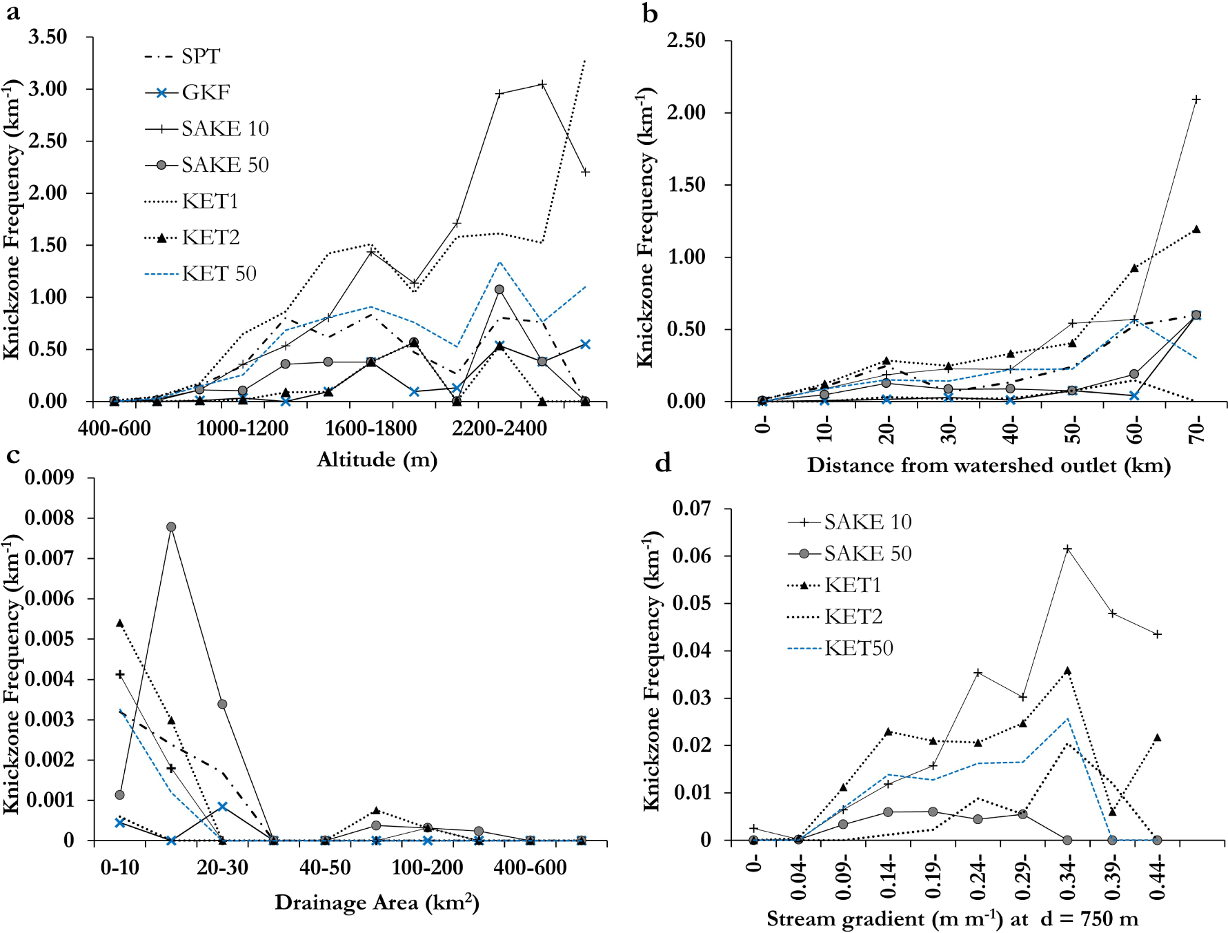
Knickzone frequency for different classes of a) altitude, b) distance from watershed outlet, c) drainage area, and d) stream gradient at location d for all bedrock rivers analyzed.
The frequency of knickzones for most methods reveals an abundance of knickzones in the smallest drainage area (10 km2; Figure 5c), although SAKE10 gives the most abundant knickzones between 10–20 km2, and KET2 does not give a clear trend because the number of knickzones is small. With an increase in stream gradient (Figure 5d), the SAKE10 result shows increasing knickzone frequency until 0.24 m m−1 but a distinct decreasing trend in reaches steeper than 0.34 m m−1. This trend is closely followed by KET2, with the highest frequency at 0.34 m m−1. In comparison, knickzones from SAKE50 increase at 0.14, 0.19, and 0.29 m m−1, respectively. The results from KET1 are similar to those from SAKE10 and SAKE50. The same is true for KET50, which follows the same trend as KET1 and uses the same scale range for the stream gradient calculation despite different DEM resolutions. In Figure 5d, KET50 follows the same trend as SAKE50 at 0.19 m m−1 and at 0.34 m m−1, respectively but both the results use a different scale range for the stream gradient calculation despite using the same DEM resolution.
4 Discussion
The knickzone distribution maps with their morphological properties with respect to bedrock rivers, such as normalized steepness index, curvature, and relative steepness index, are not only useful for landscape evolution studies but are also important to studies that (1) rely upon tectonic and climatic signals stored in stream longitudinal profiles, (2) evaluate the parameters of stream incision, and (3) examine the effects of natural barriers upon aquatic biota. Though the SPT method is time-intensive, the resulting knickzones are used in tectonic uplift studies because the exponent of drainage-area and slope relationship includes parameters that represent uplift and erosion processes [43, 44]. The channel steepness (ks), a useful index for tectonic geomorphic studies [45, 46] has been found to correlate with rates of rock uplift, exhumation, and stream incision [47]. The GKF tool is still under development. Although it can be used for analyzing and modeling gully head cut dynamics [48], it has not been fully implemented for extracting knickzones on a regional scale (Rengers, personal communication). Though SAKE calculates knickzone form parameters semi-automatically and has been used in applied studies [33, 37, 49], using SAKE over large datasets will increase computational time because of its dependence on spreadsheet software for data analysis. Moreover, increasing use of high-resolution DEMs for geomorphological studies leads to increasing calculation times and computational bottlenecks [50]. As such, improved methods of mapping and modelling of landforms are becoming a prerequisite for analyzing processes using high-resolution DEMs. Thus, the development of a fast and automated process for regional knickzone mapping is therefore significant. KET is advantageous over all other methods because it is faster and more automated, as shown by the time required for runs using both 50-m and 10-m DEMs to process large datasets as well as datasets of varying grid sizes and resolutions. In addition, increased availability of high-resolution airborne Li-DAR DEMs may increase the possibilities of false detection of knickzones. In this study KET yielded high Rd values for false knickzones especially at dam locations along the bedrock profile, which were manually eliminated.
One of the drawbacks of KET is that, similar to the SAKE method, its initial input parameters (the range of the stream gradient calculation and the threshold of Rd) used for the determination of the knickzones are defined separately with a certain criteria. Because different thresholds for knickzone extraction result in different numbers of well-defined knickzones (Figure 4e and 4f), they influence the knickzone frequency values which are essential for comparison with morphometric characteristics. For example, in Figure 5, knickzones from KET1 reveal the frequency of occurrence with respect to form properties more explicitly than the knickzones from KET2. Options for objective determination of thresholds will increase the usability of the KET for knickzones extraction and applied studies.
In addition, the scale of the initial input parameters plays a significant role in determining the accurate location of knickzones along the bedrock rivers. The minimum distance for the calculation of Gd and Rd was 30 m for the 10-m DEM but 80 m for the 50-m DEM (Table 1). If the threshold of Rd is within the input scale range for stream gradient calculation, the results are similar, even if different grid resolution DEMs are used (Figure 5d). Grid resolution, however, influences DEM derivative products such as slope and flow direction on a cell-by-cell basis [51]. In the case of knickzones extracted using a 50-m grid resolution, the aggregation of flow accumulation values have led to differences in the derivation of geomorphological properties; for example, concentrations of flow accumulation at each pixel (referred here as drainage area) increases compared to knickzones in 10-m grid resolution (Figure 5c). Advancements in mapping spatial patterns of streams, their morphometric parameters and related uncertainties [52, 53] highlight the need to measure and analyze channel forms at different grid resolutions. In this study, the ability of the grid resolutions to capture the variability in the stream gradient (Figure 5d), an important aspect that varies spatially along the river, represents the influence of multi-resolution DEMs on knickzone extraction. Moreover, the Rd values derived from stream gradients that are used for thresholding and determining knickzones are also affected. This is because the suitability of the grid size for each type of terrain and the size of the area of interest influence the lengths of the streamlines and channel slopes [54, 55], which subsequently alter not only the locations of knickzones but also their properties (Figure 5). This leads to uncertainty in the location of knickzones and their resulting distribution maps. This fact is illustrated in Figure 6, where knickzones extracted using all methods occur at similar locations, along a selected bedrock river profile, exemplifying the importance of studying the influence of multi-resolution DEMs and the locational uncertainty of knickzone distribution in the future.
![Figure 6 Comparison of results from SAKE and KET. a. Knickzone locations from the 50-m DEM (KET50 and SAKE50) and the 10-m DEM (KET1, KET2 and SAKE10) along a selected bedrock river. b. The gradient for d = 750 m derived from KET is almost the same for all grid resolutions. c. Selected profile along the study area. Note: Gradient information for SAKE50 was not available for d = 750 m because the scale range for trend gradient analysis used by Hayakawa and Oguchi [4] is different from that used in this study.](/document/doi/10.1515/geo-2017-0006/asset/graphic/j_geo-2017-0006_fig_006.png)
Comparison of results from SAKE and KET. a. Knickzone locations from the 50-m DEM (KET50 and SAKE50) and the 10-m DEM (KET1, KET2 and SAKE10) along a selected bedrock river. b. The gradient for d = 750 m derived from KET is almost the same for all grid resolutions. c. Selected profile along the study area. Note: Gradient information for SAKE50 was not available for d = 750 m because the scale range for trend gradient analysis used by Hayakawa and Oguchi [4] is different from that used in this study.
5 Conclusion
This study applied the newly developed KET to central Japan and compared the results with other existing methods of knickzone extraction like STP, GKF and SAKE. The results indicate that KET is useful for extracting knickzones by detecting anomalies in the stream length gradient. The KET performs well in detecting prominent knickzones in the upstream areas, although it is dependent on the applied threshold values, as is the case for the SAKE method. The KET is more automated and requires less time to run than the previous methods. Our analysis suggests that DEM resolutions do not significantly affect the detection of prominent knickzones, although they affect the values of some morphometric parameters. Future research should include accuracy assessments based on field validated knickzone locations. This is because KET was used for the first time in comparison with other tools, so all the methods were applied to a single study area. Currently, the tool is being applied to an ongoing research on another geologically different study area in Japan to test the transferability of the toolset in different geological settings (Figure 7).
![Figure 7 Distribution of 13 prominent knickzones extracted using KET with a threshold value of 1.42 × 10⁻⁵ m−1 from Hayakawa and Oguchi [4] on a 10-m DEM in the Kii peninsula of Japan](/document/doi/10.1515/geo-2017-0006/asset/graphic/j_geo-2017-0006_fig_007.png)
Distribution of 13 prominent knickzones extracted using KET with a threshold value of 1.42 × 10⁻⁵ m−1 from Hayakawa and Oguchi [4] on a 10-m DEM in the Kii peninsula of Japan
The recent version of the KET with a tutorial and sample data are accessible from this link: http://topography.csis.u−tokyo.ac.jp/resources/tools_ket/index.html. Any future updates of the tool and references to its applications in future studies will also be available at the above address.
Acknowledgements
This research is the result of the joint research in CSIS, The University of Tokyo (No. 591) and was supported by JSPS KAKENHI Grant Numbers 15H01782, 15K12452 and 16H01830. Timely answered queries and personal communication 15 with Francis Rengers also helped clarify concepts regarding the GIS Knickfinder tool. Constructive comments from the reviewers are highly appreciated.
Authors’ Contribution
The first author and Yuichi S. Hayakawa conceptualized KET. The first author drafted the manuscript and performed the comparative analysis. Uttam Paudel programmed KET and performed part of the comparative analysis. Takashi Oguchi and all the authors contributed to the completion of the manuscript.
References
[1] Gardner, T.W., Experimental study of knickpoint and longitudinal profile evolution in cohesive, homogeneous material. Geol Soc Am Bull, 1983, 10.1130/0016-7606 (1983) 94<664:ESOKAL>2.0.COSearch in Google Scholar
[2] Miller, J.R., The influence of bedrock geology on knickpoint development and channel-bed degradation along downcutting Streams in South-Central Indiana. J Geol, 1991, 10.1086/629519Search in Google Scholar
[3] Hayakawa, Y.S., Oguchi, T., DEM-based identification of fluvial knickzones and its application to Japanese mountain rivers. Geomorphology, 2006, 78, 90–106, 10.1016/j.geomorph.2006.01.018Search in Google Scholar
[4] Hayakawa, Y.S., Oguchi, T., GIS analysis of fluvial knickzone distribution in Japanese mountain watersheds. Geomorphology 2009, 111, 27–37, 10.1016/j.geomorph.2007.11.016Search in Google Scholar
[5] Alexandrowicz, Z., Geologically controlled waterfall types in the Outer Carpathians. Geomorphology 1994, 9, 155–165, 10.1016/0169-555X(94)90073-6Search in Google Scholar
[6] Wohl, E.E., Bedrock channel morphology in relation to erosional processes. in Tinkler, K.J., and Wohl, E.E., eds., Rivers over rock: Fluvial processes in bedrock channels: American Geophysical Union Geophysical Monograph, 1998, 107, 133–15110.1029/GM107p0133Search in Google Scholar
[7] Whipple, K.X., Bedrock rivers and the geomorphology of active orogens. Annu Rev Earth Pl Sc, 2004, 10.1146/annurev.earth.32.101802.120356Search in Google Scholar
[8] Wohl, E.E., Ikeda, H., Patterns of bedrock channel erosion on the Boso Peninsula, Japan. J Geol, 1998, 106(3), 331–34610.1086/516026Search in Google Scholar
[9] Phillips, J.D., McCormack, S., Duan, J., Russo, J.P., Schumacher, A.M., Tripathi, G.N., et al., Origin and interpretation of knickpoints in the Big South Fork River basin, Kentucky–Tennessee. Geomorphology, 2010, 114, 188–19810.1016/j.geomorph.2009.06.023Search in Google Scholar
[10] Ortega, J.A., Wohl, E., Livers, B., Waterfalls on the eastern side of Rocky Mountain National Park, Colorado, USA. Geomorphology, 2013, 198, 37–4410.1016/j.geomorph.2013.05.010Search in Google Scholar
[11] Hack, J.T., Studies of longitudinal stream profiles in Virginia and Maryland. United States Geological Survey Professional Paper, 195710.3133/pp294BSearch in Google Scholar
[12] Hack, J.T., Stream-profile analysis and stream-gradient index: U.S. Geological Survey Journal of Research, 1973, v. 1, 421–429Search in Google Scholar
[13] Bishop, P., Hoey, T.B., Jansen, J.D., Artza, I.L., Knickpoint recession rate and catchment area: The case of uplifted rivers in eastern Scotland. Earth Surf Proc Land, 2005, 30, 767–77810.1002/esp.1191Search in Google Scholar
[14] Castillo, M., Bishop, P., Jansen, J.D., Knickpoint retreat and transient bedrock channel morphology triggers by base-level fall in small bedrock river catchments: The case of the Isle of Jura, Scotland. Geomorphology, 2013 1-9, 180–18110.1016/j.geomorph.2012.08.023Search in Google Scholar
[15] Flores-Cervantes, J. H., Istanbulluoglu, E. and Bras, R.L., Development of Gullies on the Landscape: A Model of Headcut Retreat Resulting from Plunge Pool Erosion. J Geophys Res, 2006 111(F1), 1–14,10.1029/2004JF000226Search in Google Scholar
[16] Jansen, J.D., Fabel, D., Bishop, P., Xu, S., Schnabel, C., Codilean, A.T., Does decreasing paraglacial sediment supply slow knickpoint retreat? Geology, 2011, 39, 543–54610.1130/G32018.1Search in Google Scholar
[17] Pederson, J.L., Tresslor, C., Colorado River long-profile netrics, knickzones and their meaning. Earth and Planetary Science Letters, 2012, 345-348, 171-17910.1016/j.epsl.2012.06.047Search in Google Scholar
[18] Hayakawa, Y., Matsukura, Y., Recession rates of waterfalls in Boso Peninsula, Japan, and a predictive equation. Earth Surf Proc Land, 2003, 28, 675–68410.1002/esp.519Search in Google Scholar
[19] Wobus, C.W., Crosby, B.T., Whipple, K.X., Hanging valleys in fluvial systems: Controls on occurrence and implications for landscape evolution. J Geophys Res-Earth, 2006a, 111, 2003–201210.1029/2005JF000406Search in Google Scholar
[20] Lyons, N.J., Mitasova, H., Wegmann, K.W., Improving mass-wasting inventories by incorporating debris flow topographic signatures. Landslides, 2014, 11, 385–397, 10.1007/s10346-013-0398-0Search in Google Scholar
[21] Bressan, F., Papanicolaou, A., Thomas, J., Wilson, C., Elhakeem, M., Knickpoint Migration and Evolution in the Deep Loess Region of Western Iowa. In: World Environmental and Water Resources Congress, 2013, 1971–1980, 10.1061/9780784412947.193Search in Google Scholar
[22] Heimsath, A.M., Chappel, J., Dietrich, W.E., Nishiizumi, K., Finkel, R, C., Late Quaternary erosion in southeastern Australia: a field example using cosmogenic nuclides. Quaternary International, 2001, 83–85, 169–18510.1016/S1040-6182(01)00038-6Search in Google Scholar
[23] Whipple, K.X., Tucker, G.E., Dynamics of the stream-power river incision model: Implications for height limits of mountain ranges, landscape response timescales, and research needs, J Geophys Res, 1999, 104, 10.1029/1999JB900120Search in Google Scholar
[24] Ambili, V., Narayana, A.C., Tectonic effects on the longitudinal profiles of the Chaliyar River and its tributaries, southwest India. Geomorphology 2014, 217, 37–4710.1016/j.geomorph.2014.04.013Search in Google Scholar
[25] Antón, L., De Vicente, G., Muñoz-Martín, A., Stokes, M., Using river long profiles and geomorphic indices to evaluate the geomorphological signature of continental scale drainage capture, Duero basin (NW Iberia). Geomorphology 2014, 206, 250–261, 10.1016/j.geomorph.2013.09.028Search in Google Scholar
[26] Sakai, H., Causes of high-density waterfall distribution. Nature of Tokyo Metropolis, 24. Takao Natural Science Museum, Tokyo, 1998, 1–21 (In Japanese)Search in Google Scholar
[27] Zaprowski, B.J., Evenson, E.B., Pazzaglia, F.J., Epstein, J.B., Knickzone propagation in the Black Hills and northern High Plains: A different perspective on the late Cenozoic exhumation of the Laramide Rocky Mountains. Geology, 2001, 29, 547–55010.1130/0091-7613(2001)029<0547:KPITBH>2.0.CO;2Search in Google Scholar
[28] Crosby, B.T., Whipple, K.X., Knickpoint initiation and distribution within fluvial networks: 236 waterfalls in the Waipaoa River, North Island, New Zealand. Geomorphology, 2006 82, 16–3810.1016/j.geomorph.2005.08.023Search in Google Scholar
[29] Whipple, K.X., Wobus, C., Crosby, B., Kirby, E., Sheehan, D., New tools for quantitative geomorphology: extraction and interpretation of stream profiles from digital topographic data. In: Geological Society of America, Annual Meeting. NSF Geomorphology and Land Use Dynamics, Boulder Colorado, 2007Search in Google Scholar
[30] Hill, J.S., Stewart, K.G., Automatic selection of knickpoints in longitudinal river profiles using open-source R script and a combination of normalized steepness, smoothed slope, and sum of the differences. GSA Annual Meeting, 2014 (Abstract only)Search in Google Scholar
[31] Zhang, H.P., Zhang, P.Z., Fan, Q.C., Initiation and recession of the fluvial knickpoints: A case study from the Yalu River-Wangtian’e volcanic region, northeastern China. Science China Earth Sciences, 2011, 54, 1746–1753, 10.1007/s11430-011-4254-6Search in Google Scholar
[32] Wei, Z., Bi, L., Xu, Y., He, H., Evaluating knickpoint recession along an active fault for paleoseismological analysis: The Hushan Piedmont, Eastern China, Geomorphology, 2015, 235, 63–75, 10.1016/j.geomorph.2015.01.013Search in Google Scholar
[33] Yunus, A. P., Morphometric analysis of Drainage basin in Western Arabian Peninsula. Doctoral thesis for the Department of Natural Environmental Studies. Graduate School of Frontier Science, The University of Tokyo, 2015Search in Google Scholar
[34] Rengers, F., GISKnickFinder, 2012Search in Google Scholar
[35] Flint JJ. 1974. Stream Gradient as a Function of Order, Magnitude, and Discharge. Water Resources Research 10: 969-973.10.1029/WR010i005p00969Search in Google Scholar
[36] Yunus, A. P., Geomorphic and lithologic control on bedrock channels in drainage basins of the Western Arabian Peninsula. Arab J Geosci, 2016a, 9(133), 10.1007/s12517-015-2179-7Search in Google Scholar
[37] Yunus, A. P., Remote identification of fluvial knickzones and their imprints on landscape morphology in the passive margins of Western Arabia. J Arid Environ, 2016b, 130, 14–2910.1016/j.jaridenv.2016.02.016Search in Google Scholar
[38] ESRI, ArcGIS® Desktop, 2011Search in Google Scholar
[39] Tarboton, D., Terrain analysis using digital elevation models in hydrology. In: 23rd ESRI International Users Conference. San Diego, California, 2003, 1–13Search in Google Scholar
[40] Sohma, T., Kunugiza, K., The formation of the Hida nappe and the tectonics of Mesozoic sediments: the tectonic evolution of the Hida region, central Japan. Memoirs of the Geological Society of Japan, 1993, 42, 1–20Search in Google Scholar
[41] Ide, S., Complex source processes and the interaction of moderate earthquakes during the earthquake swarm in the Hida-Mountains, Japan, 1998. Tectonophysics, 2001, 334(1), 35–5410.1016/S0040-1951(01)00027-0Search in Google Scholar
[42] Hayakawa, Y.S., Spatial distribution and formation of fluvial knickzones in Japanese mountain watersheds, 2007, PhD Dissertation, Department of Earth and Planetary Science, Graduate School of Science, the University of Tokyo.Search in Google Scholar
[43] Kirby, E., Whipple, K., Quantifying differential rock-uplift rates via stream profile analysis. Geology, 2001, 29, 415–41810.1130/0091-7613(2001)029<0415:QDRURV>2.0.CO;2Search in Google Scholar
[44] Wobus, C., Whipple, K.X., Kirby, E., Snyder, N., Johnson, J., Spyropolou, K., Crosby, B., and Sheehan, D., 2006, Tectonics from topography: Procedures, promise, and pitfalls: Geological Society of America Special Papers, v. 398, p. 55-74, 10.1130/2006.2398(04)Search in Google Scholar
[45] Hoke, G.D., Graber, N.R., Mescua, J.F., Giambiagi, L.B., Fitzgerald, P.G., Metcalf, J.R., Near pure surface uplift of Argentine Frontal Cordillera: insights from (U-Th)/He thermochronometry and geomorphic analysis. From: Sepú lveda, S. A., Giambiagi, L. B., Moreiras, S. M., Pinto, L., Tunik, M., Hoke, G. D. & Farı´as, M. (eds), Geodynamic Processes in the Andes of Central Chile and Argentina. Geological Society, London, Special Publications, 2015, 399, 383–399, http://dx.doi.org/10.1144/SP399.410.1144/SP399.4Search in Google Scholar
[46] Sembroni, A., Molin, P., Pazzaglia, F.J., Faccenna, C., Abebe, B., Evolution of continental-scale drainage in response to mantle dynamics and surface processes: An example from the Ethiopian Highlands. Geomorphology, 2016, 261, 12–29, 10.1016/j.geomorph.2016.02.022Search in Google Scholar
[47] Andreani, L., Stanek, K.P., Gloaguen, R., Krentz, O., Domínguez, L. G., DEM-Based Analysis of Interactions between Tectonics and Landscapes in the Ore Mountains and Eger Rift (East Germany and NW Czech Republic). Remote Sensing, 2014, 6(9), 7971–8001, 10.3390/rs6097971Search in Google Scholar
[48] Rengers, F., Tucker, G.E., Analysis and modeling of gully headcut dynamics, North American high plains. J Geophys Res-Earth, 2014, 119, 10.1002/2013JF002962Search in Google Scholar
[49] Vatne, G., Irvine-Fynn, T.D.L., Morphological dynamics of englacial channel, Hydrol Earth Syst Sc Discuss, 2015, 12, 7615– 7664, 10.5194/hessd-12-7615-2015Search in Google Scholar
[50] Liu, K., Tang, G., Jiang, L., Zhu, A.X., Yang, J., Song, X., Regional-scale calculation of the LS factor using parallel processing. Comput Geosci, 2015, 78, 110–122, 10.1016/j.cageo.2015.02.001Search in Google Scholar
[51] Hengl, T., Finding the right pixel size. Comput Geosci, 2006, 32(9), 1283–1298, 10.1016/j.cageo.2005.11.008Search in Google Scholar
[52] Lea, D.M., Legleiter, C.J., Mapping spatial patterns of stream power and channel change along a gravel-bed river in northern Yellowstone. Geomorphology, 2016, 252, 66–79, 10.1016/j.geomorph.2015.05.033Search in Google Scholar
[53] Tantasirin, C., Nagai, M., Tipdecho, T., Tripathi, N.K., Reducing hillslope size in digital elevation models at various scales and the effects on slope gradient estimation, Geocarto International, 2016, 31(2), 140–157, 10.1080/10106049.2015.1004133Search in Google Scholar
[54] Buakhao, W., Kangrang, A., DEM Resolution Impact on the Estimation of the Physical Characteristics of Watersheds by Using SWAT. Advances in Civil Engineering, 2016, Article ID 8180158. http://dx.doi.org/10.1155/2016/818015810.1155/2016/8180158Search in Google Scholar
[55] Gallen, S.F., Wegmann, K.W., Frankel, K.L., Hughes, S., Lewis, R.Q., Lyons, N., et al., Hillslope response to knickpoint migration in the Southern Appalachians: implications for the evolution of post-orogenic landscapes. Earth Surface Processes and Landforms, 2011, 10.1002/esp.2150Search in Google Scholar
© 2017 T. Zahra et al.
This work is licensed under the Creative Commons Attribution-NonCommercial-NoDerivatives 3.0 License.
Articles in the same Issue
- Regular Articles
- Two types of gabbroic xenoliths from rhyolite dominated Niijima volcano, northern part of Izu-Bonin arc: petrological and geochemical constraints
- Regular Articles
- CRSP, numerical results for an electrical resistivity array to detect underground cavities
- Regular Articles
- Magma evolution inside the 1631 Vesuvius magma chamber and eruption triggering
- Regular Articles
- Probabilities of Earthquake Occurrences along the Sumatra-Andaman Subduction Zone
- Regular Articles
- Modelling of carrying capacity in National Park - Fruška Gora (Serbia) case study
- Regular Articles
- Knickzone Extraction Tool (KET) – A new ArcGIS toolset for automatic extraction of knickzones from a DEM based on multi-scale stream gradients
- Regular Articles
- When the display matters: A multifaceted perspective on 3D geovisualizations
- Regular Articles
- Dependence of Gully Networks on Faults and Lineaments Networks, Case Study from Hronska Pahorkatina Hill Land
- Regular Articles
- Environmental Geochemistry of Geophagic Materials from Free State Province in South Africa
- Regular Articles
- Neotectonic interpretations and PS-InSAR monitoring of crustal deformations in the Fujian area of China
- Regular Articles
- Dual-shale-content method for total organic carbon content evaluation from wireline logs in organic shale
- Regular Articles
- The dolerite dyke swarm of Mongo, Guéra Massif (Chad, Central Africa): Geological setting, petrography and geochemistry
- Regular Articles
- Seismic data filtering using non-local means algorithm based on structure tensor
- Regular Articles
- Pore Distribution Characteristics of the Igneous Reservoirs in the Eastern Sag of the Liaohe Depression
- Regular Articles
- Three-dimensional structural model of the Qaidam basin: Implications for crustal shortening and growth of the northeast Tibet
- Regular Articles
- Failure Mode of the Water-filled Fractures under Hydraulic Pressure in Karst Tunnels
- Regular Articles
- Creating a low carbon tourism community by public cognition, intention and behaviour change analysisa case study of a heritage site (Tianshan Tianchi, China)
- Regular Articles
- Mapping Mangrove Density from Rapideye Data in Central America
- Regular Articles
- Marine sediment cores database for the Mediterranean Basin: a tool for past climatic and environmental studies
- Regular Articles
- Retrofitting the Low Impact Development Practices into Developed Urban areas Including Barriers and Potential Solution
- Regular Articles
- Spatial uncertainty of a geoid undulation model in Guayaquil, Ecuador
- Regular Articles
- Structure and Filling Characteristics of Paleokarst Reservoirs in the Northern Tarim Basin, Revealed by Outcrop, Core and Borehole Images
- Regular Articles
- Ground volume assessment using ’Structure from Motion’ photogrammetry with a smartphone and a compact camera
- Regular Articles
- Classification of coal seam outburst hazards and evaluation of the importance of influencing factors
- Regular Articles
- Geochemical characterization of Neogene sediments from onshore West Baram Delta Province, Sarawak: paleoenvironment, source input and thermal maturity
- Regular Articles
- Influence of Social-economic Activities on Air Pollutants in Beijing, China
- Regular Articles
- Spectral properties of weathered and fresh rock surfaces in the Xiemisitai metallogenic belt, NW Xinjiang, China
- Regular Articles
- Geochemistry of sandstones and shales from the Ecca Group, Karoo Supergroup, in the Eastern Cape Province of South Africa: Implications for provenance, weathering and tectonic setting
- Regular Articles
- Petrology and geochemistry of meta-ultramafic rocks in the Paleozoic Granjeno Schist, northeastern Mexico: Remnants of Pangaea ocean floor
- Regular Articles
- Distal turbidite fan/lobe succession of the Late Oligocene Zuberec Fm. – architecture and hierarchy (Central Western Carpathians, Orava–Podhale basin)
- Regular Articles
- Fourier Transform Infrared Spectroscopy of Clay Size Fraction of Cretaceous-Tertiary Kaolins in the Douala Sub-Basin, Cameroon
- Regular Articles
- Optimized AVHRR land surface temperature downscaling method for local scale observations: case study for the coastal area of the Gulf of Gdańsk
- Regular Articles
- New non-linear model of groundwater recharge: Inclusion of memory, heterogeneity and visco-elasticity
- Regular Articles
- “Urban geosites” as an alternative geotourism destination - evidence from Belgrade
- Regular Articles
- A customized resistivity system for monitoring saturation and seepage in earthen levees: installation and validation
- Regular Articles
- Consideration of Landsat-8 Spectral Band Combination in Typical Mediterranean Forest Classification in Halkidiki, Greece
- Regular Articles
- Coda Wave Attenuation Characteristics for North Anatolian Fault Zone, Turkey
- Regular Articles
- Modal composition and tectonic provenance of the sandstones of Ecca Group, Karoo Supergroup in the Eastern Cape Province, South Africa
- Regular Articles
- Quantitative studies of the morphology of the south Poland using Relief Index (RI)
- Regular Articles
- Interpretation of sedimentological processes of coarse-grained deposits applying a novel combined cluster and discriminant analysis
- Regular Articles
- Utilizing borehole electrical images to interpret lithofacies of fan-delta: A case study of Lower Triassic Baikouquan Formation in Mahu Depression, Junggar Basin, China
- Regular Articles
- Grain size statistics and depositional pattern of the Ecca Group sandstones, Karoo Supergroup in the Eastern Cape Province, South Africa
- Regular Articles
- Carbonate stable isotope constraints on sources of arsenic contamination in Neogene tufas and travertines of Attica, Greece
- Regular Articles
- Appreciation of landscape aesthetic values in Slovakia assessed by social media photographs
- Regular Articles
- Geochemistry of Selected Kaolins from Cameroon and Nigeria
- Regular Articles
- Spatial pattern of ASG-EUPOS sites
- Regular Articles
- A Stream Tilling Approach to Surface Area Estimation for Large Scale Spatial Data in a Shared Memory System
- Regular Articles
- A location-based multiple point statistics method: modelling the reservoir with non-stationary characteristics
- Regular Articles
- Water Inrush Analysis of the Longmen Mountain Tunnel Based on a 3D Simulation of the Discrete Fracture Network
- Regular Articles
- A Computer Program for Practical Semivariogram Modeling and Ordinary Kriging: A Case Study of Porosity Distribution in an Oil Field
- Regular Articles
- Imaging and locating paleo-channels using geophysical data from meandering system of the Mun River, Khorat Plateau, Northeastern Thailand
- Regular Articles
- Rare earth element contents of the Lusi mud: An attempt to identify the environmental origin of the hot mudflow in East Java – Indonesia
- Regular Articles
- Is Nigeria losing its natural vegetation and landscape? Assessing the landuse-landcover change trajectories and effects in Onitsha using remote sensing and GIS
- Regular Articles
- Methodological approach for the estimation of a new velocity model for continental Ecuador