Exact and numerical solutions of the fractional Sturm–Liouville problem
-
Malgorzata Klimek
 ,
Mariusz Ciesielski
,
Mariusz Ciesielski

Abstract
In the paper, we discuss the regular fractional Sturm-Liouville problem in a bounded domain, subjected to the homogeneous mixed boundary conditions. The results on exact and numerical solutions are based on transformation of the differential fractional Sturm-Liouville problem into the integral one. First, we prove the existence of a purely discrete, countable spectrum and the orthogonal system of eigenfunctions by using the tools of Hilbert-Schmidt operators theory. Then, we construct a new variant of the numerical method which produces eigenvalues and approximate eigenfunctions. The convergence of the procedure is controlled by using the experimental rate of convergence approach and the orthogonality of eigenfunctions is preserved at each step of approximation. In the final part, the illustrative examples of calculations and estimation of the experimental rate of convergence are presented.
1 Introduction
In the paper, we study (from a theoretical and numerical point of view) the fractional Sturm-Liouville problem (FSLP) with the homogeneous mixed boundary conditions. The Sturm-Liouville problem in a fractional version can be derived by using different approaches. The first one consists of replacing the integer order derivative in the classical Sturm-Liouville problem by a fractional order derivative [1, 14]. However, this approach does not lead to orthogonal systems of eigenfunctions. The second approach is connected with the application of the calculus of variations [16, [17]. In this case, the obtained fractional differential equations can be interpreted as fractional Euler-Lagrange equations [2, 16, 18, 21, 22, 27]. They contain the differential operator, which is a composition of the left and the right fractional derivative [16, 17]. This feature leads to fundamental difficulties in calculating eigenvalues and deriving the exact solutions in a closed form, even in a simple case of a fractional oscillator problem in a bounded domain. Explicit solutions and eigenvalues are known, so far, only for a few FSLP, like fractional oscillator problem on unbounded domain [28], and for some singular cases like fractional Legendre and Jacobi problems [17, 31, 32], and fractional Bessel equation [23].
The FSLP, along with its eigenfunction’s system and eigenvalues, is connected to a fractional diffusion [19, 20] in a bounded domain. The term ‘fractional diffusion’ is to be understood as the application of fractional derivatives in description of processes of anomalous diffusion. Such diffusive processes appear in many fields of science and engineering, e.g., heat conduction in materials, fluid pressure in porous media, human migration, movement of proteins in cells, transport of lipids on cell membranes, transport on social networks, bacterial motility, and others. Classical results show that in order to solve diffusion equations in a bounded domain, one needs to apply the suitable orthogonal systems of functions, usually connected to a respective Sturm-Liouville problem. Therefore FSLPs, determined in bounded domains, are an emerging meaningful area of the fractional differential equations theory. The orthogonal eigenfunctions’ systems of FSLPs are and will be a useful tool in solving partial fractional differential equations connected to anomalous diffusion processes. Preliminary results are given in papers [17, 18, 19, 20] and show that by applying the eigenfunctions’ systems, we can study fractional diffusion problems with variable diffusivity and calculate the explicit solutions or establish the existence- uniqueness results and analyze the properties of solutions. Similar to the classical Sturm-Liouville theory, it appears that the existence of the purely discrete spectrum and the associated orthogonal eigenfunctions’ system is strongly connected to the singularity of FSLP, or in case of a regular FSLP, to the choice of boundary conditions. In paper [20], the proof was given for the regular FSLP subjected to the homogeneous Dirichlet conditions, now we shall present the result on the regular FSLP subjected to the homogeneous mixed boundary conditions. This new result is developed by converting the differential FSLP to the equivalent integral one and by applying the results of the Hilbert-Schmidt operators theory.
As we have mentioned, the problem of finding analytical solutions of the FSLP, containing both the left and right fractional derivative, is still a challenge for scientists. Therefore, numerical methods of solving the FSLP are being simultaneously developed. During the last few years, several numerical algorithms (based on direct or indirect methods) have been proposed to obtain approximate solutions of the fractional Euler-Lagrange equations [5, 6, 7, 8, 9, 10, 11, 30].
The same problem appears in calculating the eigenvalues of the FSLP. The most common approach to determine eigenvalues and eigenfunctions for Sturm-Liouville operators of integer and fractional order is to use a numerical method. The numerical solution of the Sturm-Liouville problem of integer order can be found in literature i.e. the Pruess, shooting and finite difference methods [4, 26]. In paper [29], the control volume method is used to determine the eigenvalues of the classical Sturm-Liouville problem. However, for FSLPs involving both the left and the right derivative, the adequate set of numerical tools still requires further and extensive work.
In our previous paper [12], we developed the numerical method for solving a fractional eigenvalue problem - the version of the FSLP with the homogeneous mixed boundary conditions. The proposed numerical scheme was based on the discretization of Caputo derivatives involving the boundary conditions. This approach allowed us to approximate the eigenfunctions keeping their orthogonality at each step of approximation. Moreover, the convergence was controlled by using the experimental rates of convergence formulas both for the eigenvalues and for the eigenvectors. The obtained rate of convergence was close to 1.
In paper [3], the FSLP with Dirichlet boundary conditions was considered. The authors analysed two approaches to the FSLP: discrete and continuous. They investigated the numerical solution of the FSLP by using the truncated Grunwald-Letnikov fractional derivative.
Now, we will construct a numerical scheme to calculate the approximate eigenvalues and eigenfunctions, by applying the approach presented in papers [7, 9, 11]. First, we transform the FSLP into an intermediate integral equation and then we discretize the obtained equation by using the numerical quadrature rule.. This method allows us to obtain the numerical scheme for which the experimental rate of convergence in all the considered examples tends to 2α. As we study the FSLP with order α > 1/2, we clearly see that the new numerical method gives better convergence than the one introduced in [12], while the orthogonality of the approximate eigenfunctions is also kept at each step of the procedure.
The paper is organized as follows. Section 2 presents the analyzed problem and recalls basic definitions and main properties of fractional differential and integral operators. In Section 3 the exact solution of the FSLP is depicted, while in Section 4 the numerical solution is given. Finally, in Section 5, we show numerical results for two examples of the FSLP, and we conclude the paper with a section containing brief conclusions.
2 Preliminaries
We recall the left and right Caputo fractional derivatives of order α ∈ (0, 1) (see e.g. [13, 15, 24])
and the left and right Riemann-Liouville fractional derivatives of order α ∈ (0, 1) ([13, 15, 24])
where the operators
We also recall the composition rules of fractional operators for the case of order α ∈ (0, 1]
and for the Riemann-Liouville derivatives
All the above rules are fulfilled for all x ∈ [a, b] when function y is a continuous one.
Now, we shall quote the general formulation of the fractional eigenvalue problem, introduced and investigated in papers [16, 17].
Definition 2.1
Let α ∈ (0, 1). With the notation
consider the fractional Sturm-Liouville equation (FSLE)
where p(x) ≠ 0, w(x) > 0 ∀ x ∈ [a, b] and p, q, w are real-valued continuous functions in [a, b] and boundary conditions are:
with
Let us observe that in the case α = 1 we have:
with the boundary conditions:
The aim of this paper is to study FSLP subjected to a such a set of boundary conditions that leads to a purely discrete countable spectrum and to the orthogonal eigenfunctions’ system constituting the basis in the respective weighted Hilbert space.
3 Exact solutions
In this section, we shall formulate the FSLP with an equation containing the fractional differential operator (2.11). We investigate the eigenvalues and eigenfunctions’ system connected to the FSLE in the case of order α fulfilling condition: 1 ≥ α > 1/2
subject to the mixed boundary conditions in the fractional version and on the space of continuous functions
Let us observe that the above regular FSLP is a special case of the general FSLP given in Definition 2.1 when constants c2 = d1 = 0.
We propose a transformation of the introduced differential Sturm-Liouville problem to the integral one on the subspace of continuous functions defined below:
We start by introducing the following integral operator
and we note that on the CB[a, b], subspace of continuous functions, the following relation is valid
In addition, it is easy to check that
therefore the intermediate integral form of the equation (2.12) looks as follows
In order to invert the integral operator on the left-hand side, we estimate the norm of the Tq operator in the C[a, b] space with the supremum norm ‖ ⋅ ‖ and obtain
Let us denote the parameter ξ as follows:
then the above calculations lead to the following lemma.
Lemma 3.1
Let 1 ≥ α > 1/2 and
When the norm of the Tq-operator is smaller than 1, we can invert operator 1 + Tq.
Lemma 3.2
Let 1 ≥ α > 1/2,
and the function (1 + Tq)−1Twf ∈ CB [a, b], i.e. it obeys boundary conditions (3.2).
Proof
Let us denote
and observe that for any function f ∈ C[a, b] and k ∈ ℕ
Thus, series
and we recall that for any f ∈ C[a, b] we have
and we conclude that
□
For functions f ∈ CB [a, b] we can prove the equivalence of the differential and the integral form of the fractional Sturm-Liouville problem. Namely, the following lemma is valid.
Lemma 3.3
Let 1 ≥ α > 1/2,
Proof
First, assuming that f ∈ CB [a, b] is an eigenfunction corresponding to eigenvalue λ
we obtain the equality
which leads to the integral equation
Because ξ< 1 by assumption we can apply Lemma 3.2 which means we can invert the (1 + Tq)-operator on the CB [a, b]-space
It proves the first part of the equivalence statement.
Now, we assume that the continuous function f ∈ CB [a, b] is an eigenfunction of the integral FSLP corresponding to eigenvalue
We calculate the composition 𝓛qT applying the theorem on integrating of series term by term
From the above result and from equation (3.18) we obtain the implication
Therefore, we conclude that on the CB [a, b] space the equivalence of the differential and integral FSLP (3.14) is valid. □
Next, we extend the T-operator to the
The following lemma is a Straightforward corollary from Lemma 3.2.
Lemma 3.4
Let 1 ≥ α > 1/2 andξ< 1. Then, for any functionu ∈
i.e. Tu ∈ CB[a, b].
Proof
Under assumptions of the lemma, we have Twu ∈ C[a, b] and series
Similar to the proof of Lemma 3.2, we obtain the expression for the left Riemann-Liouville derivative
and the following useful inequality is valid for any function u ∈
Thence, for k ∈ ℕ we have
and we recover the second boundary condition
□
In order to consider the spectral properties of the integral operator T, we shall convert it to the integral Hilbert-Schmidt operator. To this aim we explicitly calculate its kernel. First, we express operators Tq and Tw as integral operators with the corresponding kernels. We obtain the following formula for the kernel Kq of the Tq operator defined by Eq. (3.6)
and
with symmetric part
For the Tw operator defined by Eq. (3.4):
we calculate kernel Kw:
We now estimate the norms and values of the above kernels.
Lemma 3.5
Let 1 ≥ α > 1/2,
Proof
Let us start with the estimation of the absolute values of the Kq-kernel on square [a, b] × [a, b]:
From the above inequality we infer that estimation (3.31) is also valid. □
From the above lemma we obtain |Kw (x, s)| ≤ ξw /(b − a) and Kw ∈
Now, we reformulate the T operator given by Eq. (3.11) in the form of Hilbert-Schmidt operator with kernel K:
The next step is the explicit calculation of the kernel K and examine its properties. It appears that it can be expressed as a series of convolutions described in the lemma below.
Lemma 3.6
Let 1 ≥ α > 1/2, q,
and it fulfills conditionk ∈
Proof
First, by using the convolution properties we prove formulas for operators (Tq)nTw. For n = 1 we obtain
thus it is an integral operator with the kernel given as the convolution of the Kq and Kw kernels. Terms (Tq)nTwu, n > 1 can be expressed analogously:
where we applied the mathematical induction principle with its assumption (Tq)n−1Twu(x) =
and by means of the mathematical induction we have
We observe that at any point (x, s) ∈ [a, b] ×[a, b] we have the following estimation valid
Thence, we infer that series K is absolutely and uniformly convergent on square [a, b] × [a, b]. This fact implies that it also is convergent in the
Now, we are ready to formulate the main theorem on the integral operator T.
Theorem 3.1
Let 1 ≥ α >
Proof
The compactness of the operator T results from Lemma 3.6, i.e. the fact that K ∈
It is easy to check that
Let us now assume that 〈f, (Tq)n−1Twg〉w = 〈 (Tq)n−1Twf, g〉w. We obtain for n ∈ ℕ, by applying the mathematical induction assumption and principle, that the following equality is fulfilled
As the series K is uniformly convergent on square [a, b] ×[a, b] we infer that the partial sums sequence
Thus, from the limit theorem for integrals we get
We note that for any functions f, g ∈
The above theorem on the Hilbert-Schmidt operator T implies the following result on its spectrum and eigenfunctions.
Corollary 3.1
Let 1 ≥ α >
As the eigenfunctions of the operator T belong to the CB[a, b]-space, we can apply Lemma 3.3 on the equivalence of the differential and integral eigenvalue problem to obtain a principal result on the discrete spectrum of the studied FSLP.
Theorem 3.2
Let 1 ≥ α >
Proof
We can assume that eigenfunctions’ basis is orthonormal in the
Assuming ym is an eigenfunction corresponding to eigenvalue λm and applying the orthonormality property of eigenfunctions, we get the relation below
We use the orthonormality of eigenfunctions once again and obtain the explicit formula for coefficients alm:
Now, we can write the kernel K as the series
We know that k ∈
and we infer that (3.38) is valid. □
The assumption
Corollary 3.2
Let
and the series below is convergent
Proof
We again can assume that the basis of eigenfunctions is orthonormal in
Multiplying both sides by yn and integrating over interval [a, b] we get the relation below
which leads to the following formula for eigenvalue λn
Now, we use the fact that each eigenfunction fulfills the homogeneous mixed boundary conditions and by applying the fractional integration by parts rule we arrive at the equality
Clearly, the first term on the right-hand side is positive, therefore the following inequality is valid:
which means
because we have assumed 〈 yn, yn〉w = 1.
The proven inequality means that in the case when function p is positive we have at least a finite number of negative eigenvalues and an infinite number of positive ones tending to infinity. Numbering the negative eigenvalues by n = −n0,…, −1, we get the convergence in Eq. (3.40) from the general formula (3.38). □
The proof of the analogous result for p negative is similar so we just formulate the corollary as follows noting that here we have at least a finite number of positive eigenvalues and an infinite number of the negative ones tending to −∞.
Corollary 3.3
Let
and the series below is convergent
Finally, let us note that the above statements on the regular FSLP with the fractional Sturm-Liouville operator defined in Eq. (2.11) are also valid for its reflected version with FSLO in the form of
and boundary conditions
As the proof of the result on spectrum and eigenfunctions’ system of the reflected FSLP is very simple and based only on the properties of the reflection operator in interval [a, b] we formulate the theorem omitting the proof.
Theorem 3.3
Let
4 Numerical solution
We start the construction of numerical scheme by dividing the considered interval [a, b] into N equidistant subintervals of length Δx = (b − a)/N with the central points xi = a + (i − 0.5)Δx for i = 1,…, N. A value of function y at node xi we denote as yi = y(xi). In addition, we introduce the notation xi ± 0.5 = xi ± 0.5Δx.
The intermediate integral equation Eq. (3.7) can be written as follows
with kernel K1 given by Eq. (3.27). Next, we approximate the above integrals by the quadrature rule
where uk are the weights of the quadrature rule (for the midpoint rectangular rule: uk = Δx).
If we evaluate the equation at every node xi, i = 1,…, N, then we obtain the following system of N linear algebraic equations
which can be written in the short notation for node values of eigenfunctions looks as follows:
where (K1)i, k = K1 (xi, xk).
Now, the above system of equations can be rewritten in the matrix form [25]. We introduce:
two diagonal matrices Q and W:
where
the matrix M:
for i = 1,…., N and k = 1,…., N,
the vector Y:
By using these notations, the system of equations (4.4) takes the following matrix form
and after transformations it is a matrix eigenvalue problem:
where
In order to compute the eigenvalues and eigenvectors of Eq. (4.10) one can use mathematical software. Let us note that the eigenvectors corresponding to distinct eigenvalues are orthogonal in a N-dimensional weighted Hilbert space with the scalar product defined as follows:
In calculations demonstrating the orthogonality of eigenvectors, we apply the fact that matrix M is symmetric. Let eigenvector Yλ correspond to eigenvalue λ and Yρ correspond to eigenvalue ρ. First, we have the following relation valid:
Now, we calculate the scalar products on the left- and right-hand side of the above equality remembering that Yλ and Yρ are eigenvectors of matrix A:
Subtracting the above equalities we arrive at the result
which implies that when eigenvalues are distinct, the corresponding eigenvectors are orthogonal:
In the next step, we construct the approximate eigenfunctions by applying the eigenvectors obtained via the numerical scheme corresponding to the equidistant partition of interval [a, b] into N subintervals:
Let us note that from the orthogonality of eigenvectors the lemma on approximate eigenfunctions results.
Lemma 4.1
Approximate eigenfunctions corresponding to distinct eigenvalues are orthogonal in the
Proof
The orthogonality of approximate eigenfunctions is a straightforward result of the orthogonality of eigenvectors (4.13):
□
If we assume in the considered FSLP the coefficient and weight functions constant: p = w = 1 and q = 0, then matrix A is determined by simple formula
where M = {Mi, k} = {uk(K0)i, k} = {ukK0 (xi, xk)}, for i = 1,…., N, k = 1,…., N. Let us point out that in this case kernel K0 and therefore matrix M−1 can be calculated explicitly.
4.1 The special case for functions
p(x) = w(x) = 1 andq(x) = 0. Now, we consider the mentioned special case which extends the classical harmonic oscillator equation and eigenvalue problem. Namely, we choose q = 0 and we assume that the coefficient and weight functions are constant: p = w = 1. We shall calculate exact values of the kernel and apply them further in calculating the numerical solutions. In this case, Eq. (3.7) reduces to the following form
and the composition of integral operators can be written as
where the kernel K0 (defined by Eq. (3.27) for p = 1) for order 1 ≥ α > 1/2 is of the following explicit form
For x = s (by using properties of the hypergeometric function 2F1) one has
One can see that kernel K0 is a symmetric function on square [a, b] × [a, b]
For order α = 1 we obtain
5 Example of calculations
In order to verify the proposed numerical method, we present two examples of numerical calculations of eigenvalues and eigenfunctions. As the first example we consider the generalization of the classical harmonic oscillator problem with p = w = 1 and q = 0 (this corresponds to the case studied in Subsection 4.1), and in the second example, we assumed the functions to be p(x) = x2 + exp(x), q(x) =
In Tables 1 and 2 we present the numerical values of the first ten eigenvalues for orders α ∈ {1, 0.8, 0.6} and different values of N ∈ {250, 500, 1000, 2000, 4000}. While, in Figures 1 and 2 we show graphs of the approximate eigenfunctions corresponding to the first four eigenvalues for the considered cases, respectively, and N = 4000. The approximate eigenfunctions were normalized by
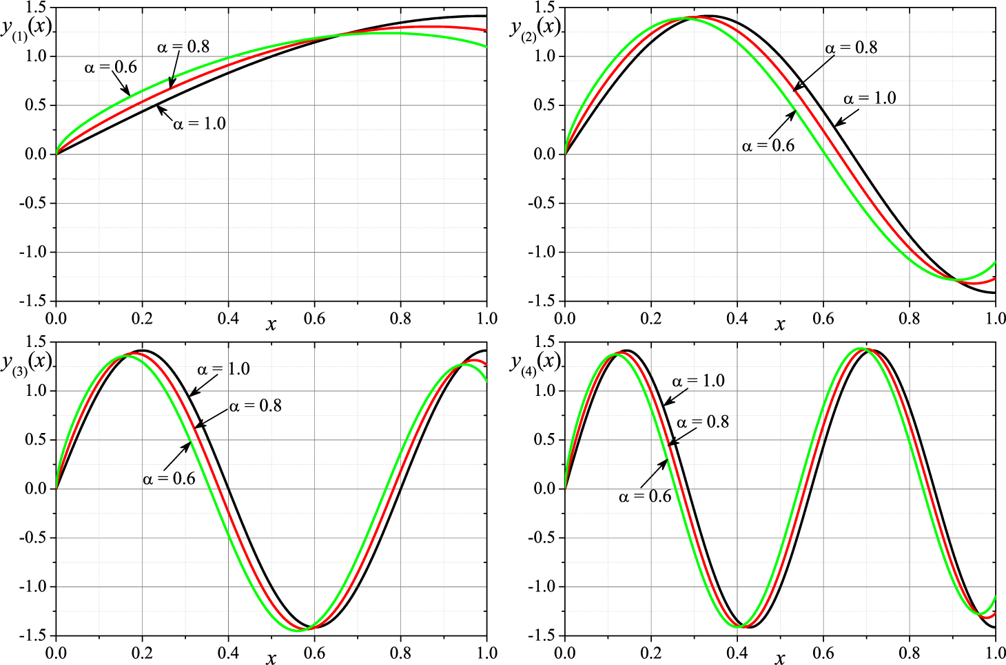
Eigenfunctions for the first 4 eigenvalues for p(x) = 1, q(x) = 0, w(x) = 1 and α ∈ {1, 0.8, 0.6} (a = 0, b = 1) (classical fractional oscillator)
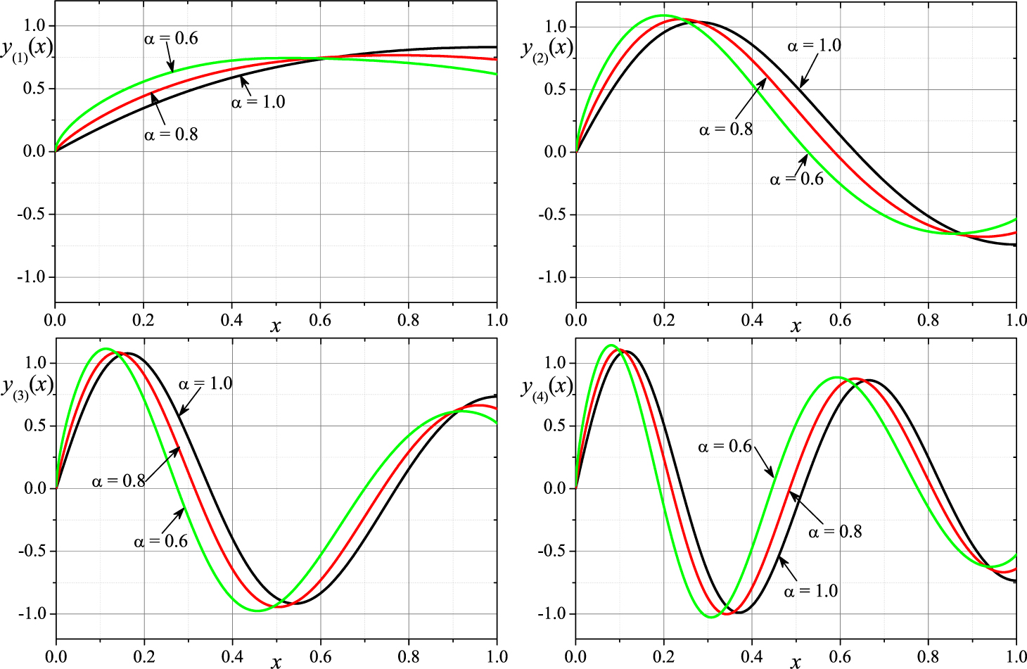
Eigenfunctions for the first 4 eigenvalues for p(x) = x2 + exp(x), q(x) =
Numerical values of the first 8 eigenvalues and the experimental rates of convergence ercλ for α ∈ {1, 0.8, 0.6}, p(x) = 1, q(x) = 0, and w(x) = 1
| α = 1 | α = 0.8 | α = 0.6 | |||||
|---|---|---|---|---|---|---|---|
| k | N | λ(k) | ercλ | λ(k) | ercλ | λ(k) | ercλ |
| 1 | 250 | 2.4673930 | - | 1.9580409 | - | 1.5966035 | - |
| 500 | 2.4673991 | 2.000 | 1.9581331 | 1.607 | 1.5989630 | 1.198 | |
| 1000 | 2.4674006 | 1.995 | 1.9581633 | 1.605 | 1.5999915 | 1.199 | |
| 2000 | 2.4674010 | 1.660 | 1.9581733 | 1.604 | 1.6004394 | 1.200 | |
| 4000 | 2.4674011 | - | 1.9581766 | - | 1.6006344 | - | |
| 2 | 250 | 22.205952 | - | 11.994294 | - | 6.4004171 | - |
| 500 | 22.206446 | 2.000 | 11.997725 | 1.603 | 6.4384921 | 1.189 | |
| 1000 | 22.206569 | 2.000 | 11.998854 | 1.603 | 6.4551977 | 1.195 | |
| 2000 | 22.206600 | 1.997 | 11.999225 | 1.602 | 6.4624940 | 1.198 | |
| 4000 | 22.206607 | - | 11.999348 | - | 6.4656744 | - | |
| 3 | 250 | 61.679954 | - | 26.986045 | - | 11.608982 | - |
| 500 | 61.683759 | 2.000 | 27.003363 | 1.602 | 11.734829 | 1.178 | |
| 1000 | 61.684710 | 2.000 | 27.009070 | 1.602 | 11.790437 | 1.191 | |
| 2000 | 61.684948 | 1.999 | 27.010950 | 1.601 | 11.814799 | 1.196 | |
| 4000 | 61.685008 | - | 27.011570 | - | 11.825433 | - | |
| 4 | 250 | 120.88317 | - | 46.289229 | - | 17.275740 | - |
| 500 | 120.89778 | 2.000 | 46.340141 | 1.600 | 17.555896 | 1.167 | |
| 1000 | 120.90144 | 2.000 | 46.356931 | 1.601 | 17.680642 | 1.186 | |
| 2000 | 120.90235 | 2.000 | 46.362466 | 1.601 | 17.735481 | 1.194 | |
| 4000 | 120.90258 | - | 46.364290 | - | 17.759454 | - | |
| 5 | 250 | 199.80624 | - | 69.085904 | - | 23.092775 | - |
| 500 | 199.84617 | 2.000 | 69.199264 | 1.599 | 23.596078 | 1.156 | |
| 1000 | 199.85616 | 2.000 | 69.236685 | 1.601 | 23.821973 | 1.181 | |
| 2000 | 199.85866 | 2.000 | 69.249025 | 1.601 | 23.921631 | 1.192 | |
| 4000 | 199.85928 | - | 69.253093 | - | 23.965264 | - | |
| 6 | 250 | 298.43670 | - | 95.198549 | - | 29.105802 | - |
| 500 | 298.52582 | 2.000 | 95.413812 | 1.598 | 29.909873 | 1.144 | |
| 1000 | 298.54811 | 2.000 | 95.484937 | 1.600 | 30.273754 | 1.175 | |
| 2000 | 298.55368 | 2.000 | 95.508401 | 1.601 | 30.434883 | 1.189 | |
| 4000 | 298.55507 | - | 95.516137 | - | 30.505545 | - | |
| 7 | 250 | 416.75900 | - | 124.20624 | - | 35.176421 | - |
| 500 | 416.93283 | 2.000 | 124.57277 | 1.596 | 36.357661 | 1.132 | |
| 1000 | 416.97630 | 2.000 | 124.69399 | 1.599 | 36.896741 | 1.170 | |
| 2000 | 416.98716 | 2.000 | 124.73400 | 1.600 | 37.136358 | 1.187 | |
| 4000 | 416.98988 | - | 124.74719 | - | 37.241618 | - | |
| 8 | 250 | 554.75442 | - | 156.01634 | - | 41.335872 | - |
| 500 | 555.06252 | 2.000 | 156.59492 | 1.595 | 42.976638 | 1.119 | |
| 1000 | 555.13956 | 2.000 | 156.78647 | 1.599 | 43.731895 | 1.164 | |
| 2000 | 555.15883 | 2.000 | 156.84971 | 1.600 | 44.068916 | 1.184 | |
| 4000 | 555.16364 | - | 156.87057 | - | 44.217221 | - | |
Numerical values of the first 8 eigenvalues and the experimental rates of convergence ercλ for α ∈ {1, 0.8, 0.6}, p(x) = x2 + exp(x), q(x) =
| α = 1 | α = 0.8 | α = 0.6 | |||||
|---|---|---|---|---|---|---|---|
| k | N | λ(k) | ercλ | λ(k) | ercλ | λ(k) | ercλ |
| 1 | 250 | 1.3584974 | - | 1.1387715 | - | 0.9893191 | - |
| 500 | 1.3584988 | 1.999 | 1.1388057 | 1.606 | 0.9903662 | 1.199 | |
| 1000 | 1.3584992 | 2.007 | 1.1388169 | 1.604 | 0.9908223 | 1.200 | |
| 2000 | 1.3584993 | 1.775 | 1.1388206 | 1.603 | 0.9910208 | 1.200 | |
| 4000 | 1.3584993 | - | 1.1388218 | - | 0.9911072 | - | |
| 2 | 250 | 17.415682 | - | 9.5114080 | - | 5.0943056 | - |
| 500 | 17.416073 | 2.000 | 9.5142567 | 1.602 | 5.1267401 | 1.188 | |
| 1000 | 17.416170 | 2.000 | 9.5151948 | 1.602 | 5.1409749 | 1.195 | |
| 2000 | 17.416195 | 1.998 | 9.5155039 | 1.601 | 5.1471929 | 1.198 | |
| 4000 | 17.416201 | - | 9.5156058 | - | 5.1499036 | - | |
| 3 | 250 | 49.362322 | - | 21.578465 | - | 9.2190735 | - |
| 500 | 49.365493 | 2.000 | 21.592998 | 1.601 | 9.3256384 | 1.178 | |
| 1000 | 49.366286 | 2.000 | 21.597789 | 1.601 | 9.3727246 | 1.191 | |
| 2000 | 49.366485 | 2.000 | 21.599368 | 1.601 | 9.3933541 | 1.196 | |
| 4000 | 49.366534 | - | 21.599888 | - | 9.4023590 | - | |
| 4 | 250 | 97.153196 | - | 37.129314 | - | 13.762621 | - |
| 500 | 97.165512 | 2.000 | 37.172412 | 1.600 | 14.001140 | 1.167 | |
| 1000 | 97.168591 | 2.000 | 37.186630 | 1.601 | 14.107352 | 1.186 | |
| 2000 | 97.169361 | 2.000 | 37.191318 | 1.601 | 14.154046 | 1.194 | |
| 4000 | 97.169554 | - | 37.192864 | - | 14.174459 | - | |
| 5 | 250 | 160.88338 | - | 55.433830 | - | 18.367541 | - |
| 500 | 160.91720 | 2.000 | 55.529924 | 1.599 | 18.795232 | 1.156 | |
| 1000 | 160.92565 | 2.000 | 55.561652 | 1.600 | 18.987191 | 1.181 | |
| 2000 | 160.92777 | 2.000 | 55.572118 | 1.600 | 19.071880 | 1.192 | |
| 4000 | 160.92830 | - | 55.575569 | - | 19.108960 | - | |
| 6 | 250 | 240.52999 | - | 76.439512 | - | 23.143959 | - |
| 500 | 240.60564 | 2.000 | 76.622406 | 1.597 | 23.828700 | 1.144 | |
| 1000 | 240.62455 | 2.000 | 76.682845 | 1.600 | 24.138585 | 1.175 | |
| 2000 | 240.62928 | 2.000 | 76.702787 | 1.600 | 24.275809 | 1.189 | |
| 4000 | 240.63046 | - | 76.709365 | - | 24.335990 | - | |
| 7 | 250 | 336.07766 | - | 99.73969 | - | 27.942888 | - |
| 500 | 336.22542 | 2.000 | 100.05127 | 1.596 | 28.948387 | 1.132 | |
| 1000 | 336.26237 | 2.000 | 100.15432 | 1.599 | 29.407255 | 1.170 | |
| 2000 | 336.27161 | 2.000 | 100.18834 | 1.600 | 29.611222 | 1.187 | |
| 4000 | 336.27391 | - | 100.19956 | - | 29.700823 | - | |
| 8 | 250 | 447.51002 | - | 125.31117 | - | 32.816924 | - |
| 500 | 447.77215 | 2.000 | 125.80346 | 1.595 | 34.214801 | 1.119 | |
| 1000 | 447.83769 | 2.000 | 125.96645 | 1.599 | 34.858243 | 1.164 | |
| 2000 | 447.85408 | 2.000 | 126.02027 | 1.600 | 35.145375 | 1.184 | |
| 4000 | 447.85818 | - | 126.03803 | - | 35.271729 | - | |
Also, in Tables 1 and 2, the experimental rate of convergence (ercλ) of numerical calculations of the k-th eigenvalue is presented. The values of ercλ for fixed parameters α and variable values of N we determined from the following formula ([12])
Analyzing the values in Tables 1 and 2, one can observe that the values of ercλ depends on the fractional order α and does not depend on the various types of functions p, q, and w and it is close to the value of 2 α.
6 Conclusions
In the paper, we studied the regular FSLP in a bounded domain, subjected to the homogeneous mixed boundary conditions. We transformed the analyzed problem into an integral one. Then, we proved the existence of a purely discrete, countable spectrum and the orthogonal system of eigenfunctions by utilizing the Hilbert-Schmidt operators theory. In the numerical approach to the FSLP, we made the discretization of the integral equation by using the numerical quadrature rule to the approximation of the integral. The obtained system of algebraic equations was rewritten as the matrix equation, from which the eigenvalues and eigenvectors are determined by using standard methods. The presented procedure allows us to calculate the approximate eigenvalues and eigenfunctions. We presented the obtained eigenvalues and eigenfunctions, for the selected functions p, q, w and the order α, to show the influence of these parameters on the solution to the considered FSLP. We also determined the experimental rate of convergence of the proposed method. The experimental rate of convergence of the numerical scheme, in all considered examples, is close to 2α. Moreover, orthogonality of the approximate eigenfunctions is kept at each step of the procedure. It should be pointed out that the presented numerical method can be treated as an extension of method used for the solution of the Sturm-Liouville problem of the integer order and, of course, for α = 1 we obtain the approximate eigenvalues and eigenfunctions for the classical Sturm-Liouivlle problem.
References
[1] Q.M. Al-Mdallal, An efficient method for solving fractional Sturm-Liouville problems. Chaos Solitons Fractals40, No 1 (2009), 183–189; 10.1016/j.chaos.2007.07.041.Search in Google Scholar
[2] O.P. Agrawal, M. M. Hasan, X. W. Tangpong, A numerical scheme for a class of parametric problem of fractional variational calculus. J. Comput. Nonlinear Dyn. 7 (2012), # 021005-1–021005-6; 10.1115/1.4005464.Search in Google Scholar
[3] R. Almeida, A.B. Malinowska, M.L. Morgado, T. Odzijewicz, Variational methods for the solution of fractional discrete/continuous Sturm-Liouville problems. J. of Mechanics of Materials and Structures12, No 1 (2017), 3–21; 10.2140/jomms.2017.12.3.Search in Google Scholar
[4] F.V. Atkinson, Discrete and Continuous Boundary Value Problems. Academic Press, New York, London (1964).10.1063/1.3051875Search in Google Scholar
[5] D. Baleanu, J.H. Asad, I. Petras, Fractional Bateman-Feshbach Tikochinsky oscillator. Commun. Theor. Phys. 61 (2014), 221–225; 10.1088/0253-6102/61/2/13.Search in Google Scholar
[6] T. Blaszczyk, M. Ciesielski, M. Klimek, J. Leszczynski, Numerical solution of fractional oscillator equation. Appl. Math. Comput. 218 (2011), 2480–2488; 10.1016/j.amc.2011.07.062.Search in Google Scholar
[7] T. Blaszczyk, M. Ciesielski, Numerical solution of fractional Sturm-Liouville equation in integral form. Fract. Calc. Appl. Anal., 17, No 2 (2014), 307–320; 10.2478/s13540-014-0170-8; https://www.degruyter.com/view/j/fca.2014.17.issue-2/issue-files/fca.2014.17.issue-2.xml.Search in Google Scholar
[8] T. Blaszczyk, A numerical solution of a fractional oscillator equation in a non-resisting medium with natural boundary conditions. RomanianReports in Phys. 67, No 2 (2015), 350–358.Search in Google Scholar
[9] T. Blaszczyk, M. Ciesielski, Fractional oscillator equation - transformation into integral equation and numerical solution. Appl. Math. Comput. 257 (2015), 428–435; 10.1016/j.amc.2014.12.122.Search in Google Scholar
[10] L. Bourdin, J. Cresson, I. Greff, P. Inizan, Variational integrator for fractional Euler-Lagrange equations. Appl. Numer. Math. 71 (2013), 14–23; 10.1016/j.apnum.2013.03.003.Search in Google Scholar
[11] Ciesielski M., Blaszczyk T., Numerical solution of non-homogenous fractional oscillator equation in integral form. J. of Theoretical andApplied Mechanics53, No 4 (2015), 959–968.10.15632/jtam-pl.53.4.959Search in Google Scholar
[12] M. Ciesielski, M. Klimek, T. Blaszczyk, The fractional Sturm-Liouville Problem – Numerical approximation and application in fractional diffusion. J. of Computational and Applied Math. 317, (2017), 573–588; 10.1016/j.cam.2016.12.014.Search in Google Scholar
[13] K. Diethelm, The Analysis of Fractional Differential Equations. Lecture Notes in Mathematics Vol. 2004, Springer-Verlag (2010).10.1007/978-3-642-14574-2Search in Google Scholar
[14] M.A. Hajji, Q.M. Al-Mdallal, F.M. Allan, An efficient algorithm for solving higher-order fractional Sturm-Liouville eigenvalue problems. J. Comput. Phys. 272, (2014), 550–558; 10.1016/j.jcp.2014.04.048.Search in Google Scholar
[15] A.A. Kilbas, H.M. Srivastava, J.J. Trujillo, Theory and Applications of Fractional Differential Equations. Elsevier, Amsterdam (2006).Search in Google Scholar
[16] M. Klimek, O.P. Agrawal, On a regular fractional Sturm–Liouville problem with derivatives of order in (0, 1). In: Proc. of the 13th International Carpathian Control Conf., Vysoke Tatry (2012); 10.1109/CarpathianCC.2012.6228655.Search in Google Scholar
[17] M. Klimek, O.P. Agrawal, Fractional Sturm-Liouville problem. Comput. Math. Appl. 66 (2013), 795–812; 10.1016/j.camwa.2012.12.011.Search in Google Scholar
[18] M. Klimek, T. Odzijewicz, A.B. Malinowska, Variational methods for the fractional Sturm-Liouville problem. J. Math. Anal. Appl. 416, No 1 (2014), 402–426; 10.1016/j.jmaa.2014.02.009.Search in Google Scholar
[19] M. Klimek, Fractional Sturm-Liouville problem and 1D space-time fractional diffusion problem with mixed boundary conditiond. In: Proc. of the ASME 2015 Internat. Design Engineering Technical Conf. (IDETC) and Computers and Information in Engineering Conf. (CIE), Boston (2015); 10.1115/DETC2015-46808.Search in Google Scholar
[20] M. Klimek, A.B. Malinowska, T. Odzijewicz, Applications of the fractional Sturm-Liouville problem to the space-time fractional diffusion in a finite domain. Fract. Calc. Appl. Anal. 19, No 2 (2016), 516–550; 10.1515/fca-2016-0027; https://www.degruyter.com/view/j/fca.2016.19.issue-2/issue-files/fca.2016.19.issue-2.xml.Search in Google Scholar
[21] A.B. Malinowska, D.F.M. Torres, Introduction to the Fractional Calculus of Variations. Imperial College Press, London (2012).10.1142/p871Search in Google Scholar
[22] A.B. Malinowska, T. Odzijewicz, D.F.M. Torres, Advanced Methods in the Fractional Calculus of Variations. Springer Internat. Publ., London (2015).10.1007/978-3-319-14756-7Search in Google Scholar
[23] M. d’Ovidio, From Sturm-Liouville problems to to fractional and anomalous diffusions. Stochastic Process. Appl. 122 (2012), 3513–3544; 10.1016/j.spa.2012.06.002.Search in Google Scholar
[24] I. Podlubny, Fractional Differential Equations. Academic Press, San Diego (1999).Search in Google Scholar
[25] I. Podlubny, Matrix approach to discrete fractional calculus. Fract. Calc. Appl. Anal. 3, No 4 (2000), 359–386.Search in Google Scholar
[26] J.D. Pryce, Numerical Solution of Sturm-Liouville Problems. Oxford Univ. Press, London (1993).Search in Google Scholar
[27] F. Riewe, Nonconservative Lagrangian and Hamiltonian mechanics. Phys. Rev. E53 (1996), 1890–1899; 10.1103/PhysRevE.53.1890.Search in Google Scholar PubMed
[28] M. Rivero, J.J. Trujillo, M.P. Velasco, A fractional approach to the Sturm-Liouville problem. Cent. Eur. J. Phys. 11, No 10 (2013), 1246– 1254; 10.2478/s11534-013-0216-2.Search in Google Scholar
[29] J. Siedlecki, M. Ciesielski, T. Blaszczyk, The Sturm-Liouville eigen-value problem - a numerical solution using the control volume method. J. Appl. Math. Comput. Mech. 15, No 2 (2016), 127–136; 10.17512/jamcm.2016.2.14.Search in Google Scholar
[30] Y. Xu, O.P. Agrawal, Models and numerical solutions of generalized oscillator equations. J. Vib. Acoust. 136, No 5 (2014), Article ID 050903; 10.1115/1.4027241.Search in Google Scholar
[31] M. Zayernouri, G.E. Karniadakis, Fractional Sturm–Liouville eigen-problems: theory and numerical approximation. J. Comput. Phys. 252 (2013), 495–517; 10.1016/j.jcp.2013.06.031.Search in Google Scholar
[32] M. Zayernouri, M. Ainsworth, G.E. Karniadakis, Tempered fractional Sturm–Liouville eigenproblems. SIAM J. Sci. Computing37, No 4 (2015), A1777–A1800; 10.1137/140985536.Search in Google Scholar
© 2018 Diogenes Co., Sofia
Articles in the same Issue
- Frontmatter
- Editorial Note
- FCAA related news, events and books (FCAA–volume 21–1–2018)
- Survey Paper
- From continuous time random walks to the generalized diffusion equation
- Survey Paper
- Properties of the Caputo-Fabrizio fractional derivative and its distributional settings
- Research Paper
- Exact and numerical solutions of the fractional Sturm–Liouville problem
- Research Paper
- Some stability properties related to initial time difference for Caputo fractional differential equations
- Research Paper
- On an eigenvalue problem involving the fractional (s, p)-Laplacian
- Research Paper
- Diffusion entropy method for ultraslow diffusion using inverse Mittag-Leffler function
- Research Paper
- Time-fractional diffusion with mass absorption under harmonic impact
- Research Paper
- Optimal control of linear systems with fractional derivatives
- Research Paper
- Time-space fractional derivative models for CO2 transport in heterogeneous media
- Research Paper
- Improvements in a method for solving fractional integral equations with some links with fractional differential equations
- Research Paper
- On some fractional differential inclusions with random parameters
- Research Paper
- Initial boundary value problems for a fractional differential equation with hyper-Bessel operator
- Research Paper
- Mittag-Leffler function and fractional differential equations
- Research Paper
- Complex spatio-temporal solutions in fractional reaction-diffusion systems near a bifurcation point
- Research Paper
- Differential and integral relations in the class of multi-index Mittag-Leffler functions