From continuous time random walks to the generalized diffusion equation

1 Introduction

Brownian motion, the classical model for normal diffusion, can be explained within random walk theory according to which the particle in equal time intervals performs steps in random direction (left or right) to the nearest neighbor site. From the master equation for such a stochastic process one can find that the probability density function (PDF) W(x, t) to find the particle at position x at time t satisfies the standard diffusion equation in the continuum limit. The corresponding solution for a point initial condition is the well-known Gaussian PDF, and the mean squared displacement (MSD) has a linear dependence on time. The continuous time random walk model (CTRW) represents a generalization of the Brownian random walk model. The mathematical theory of CTRW was developed by Montroll and Weiss (1965) [34], and first applied to physical problems by Scher and Lax (1973) [52]. Nowadays it has become a very popular framework for the description of anomalous, non-Brownian diffusion in complex systems, and even after its 50 years’ history the model is still trendy with applications in various fields [23]. The Brownian random walk model is the limit case of CTRW when the waiting time PDF ψ(t) is of Poisson form and the jump length PDF λ(x) is of Gaussian form. Moreover, in the more general case of any finite characteristic waiting time T = ∫0∞tψ(t) dt and any finite jump length variance Σ² = ∫−∞∞x²λ(x) dx, the corresponding process in the diffusion limit shows normal diffusive behavior with Gaussian PDF W(x, t), [19].

It has been shown that the CTRW process with a scale-free waiting time PDF of power-law form ψ(t) ≃ t^−1−α with 0 < α < 1, leads in the continuum limit to the time fractional diffusion equation, represented by a power-law dependence of the MSD on time of form 〈 x²(t)〉 ≃ t^α [1], 33]. Since 0 < α < 1 this process is subdiffusive. Processes for which the anomalous diffusion exponent is α > 1, are superdiffusive. An example is the case of Lévy walks with long tailed jump length PDF λ(x) ≃ |x|^−1−μ, μ < 2, and spatiotemporal coupling [33]. Anomalous diffusion, either subdiffusion or superdiffusion, has been observed, for example, in the charge carrier motion in amorphous semiconductors [54], in aquifer problems [53], in living biological cells [62], including superdiffusion [2, 43] and subdiffusion [14, 21], in weakly chaotic systems [20, 60], or turbulence [44], to name a few. Furthermore, from the CTRW theory one may obtain distributed order fractional diffusion equations for ultraslow diffusive processes [4, 6, 7], where the MSD has logarithmic dependence on time found for Sinai-type disorder [57, ageing CTRW [24] or interacting subdiffusive CTRW-walkers, [45].

In this work we consider a CTRW model whose corresponding diffusion equation is of general form in the Riemann-Liouville sense. In Section 2 we provide an introduction to the generalized derivatives in the Riemann-Liouville and Caputo sense. We derive the generalized diffusion equation in the Riemann-Liouville sense from the CTRW model in Section 3. Several special cases of the model are analyzed in Section 4. In Section 5 we compare the generalized diffusion equation in normal and modified form, and we show under which conditions both equations are equivalent. A summary is given in Section 6.

2 Generalized derivatives and Mittag-Leffler functions

A string of recent works that were summarized and discussed in [36, 63] concerned definitions of new operators of fractional calculus. Some of the newly introduced derivatives belong to a class of generalized derivatives with memory kernels either in modified (or Riemann-Liouville (R-L)) form

or in the normal (or Caputo) form

The R-L fractional derivative is a special case of the generalized derivative (2.1) in which the memory kernel is of power-law form η(t) = t^−α/Γ(1 − α), 0 < α < 1, [40],

Similarly, the Caputo fractional derivative is a special case of the generalized derivative (2.2) for γ(t) = t^−α/Γ(1 − α), 0 < α < 1, [40],

As we will see later, the distributed order and tempered fractional derivatives are special cases of these generalized derivatives (2.1) and (2.2) as well. An extensive study of the generalized derivatives is presented by Kochubei [22], Luchko and Yamamoto [26], and Sandev et al. [46, 47, 49], to name but a few. Such generalized derivatives have been used in anomalous diffusion modeling by fractional and generalized Langevin equations with memory kernels of power-law, exponential, Mittag-Leffler, and tempered form, or combinations thereof [27, 28, 41, 48, 50, 51, 58, 64, 65, 66].

The famed Mittag-Leffler (M-L) functions play an important role in the theory of fractional and generalized differential equations. Here we consider the three parameter M-L function, introduced by Prabhakar [42] as follows:

where (δ)_k = Γ(δ + k)/Γ(δ) is the Pochhammer symbol. The more familiar one parameter M-L function E_α(z) and the two parameter M-L function E_α,β(z) are special cases of the three parameter M-L function for β = δ = 1 and δ = 1, respectively, see e.g. [8, 29, 40]. Introducing the Laplace transform of a function f(t) as f̂(s) = 𝓛_s[f(t)] = ∫0∞f(t)e^−st dt, for the three parameter M-L function (2.5) we get [42]

The three parameter M-L function has many applications in the description of anomalous diffusion and non-exponential relaxation processes, see for example [11, 12, 13, 15, 46, 47, 49, 51, 61].

There are many generalizations of the M-L function. We will use here the multinomial M-L function [25] defined by

where

are the so-called multinomial coefficients. This function has been shown to play an important role in description of the MSD of anomalous diffusion processes [46, 47, 50].

3 CTRW theory and subordination

Here we give a brief introduction to the fundamental results of the continuous time random walk (CTRW) theory. This stochastic model is based on the fact that individual jumps are separated by independent, random waiting times. For the PDF W(x, t) a simple algebraic form for the Fourier-Laplace transform W^~(k, s) = 𝓕_k[𝓛_s[W(x, t)]] can be found. We note that the Fourier transform of f(x) is given by F̃(k) = 𝓕[f(x)] = ∫−∞∞f(x)e^ıkx dx, and the inverse Fourier transform is defined by f(x) = 𝓕⁻¹[F̃(k)] = 12π∫−∞∞F̃(k)e^−ıkx dk. With these definitions, one finds for the PDF in the Fourier-Laplace space [33, 54]

Here ψ̂(s) is the Laplace transform of the waiting time PDF ψ(t), and λ̃(k) is the Fourier transform of the jump length PDF λ(x). The Fourier transform of the Gaussian distribution of jump lengths with variance σ² is 1−12σ²k² for small k, where σ² has the dimension of length. To avoid dimensions, we set σ² = 2. Therefore, in this paper we assume λ̃(k) ≃ 1 − k², [33]. As it was already mentioned in the Introduction, the CTRW process with a scale-free waiting time PDF of a power law form ψ(t) ≃ t^−1−α, 0 < α < 1, and Gaussian distribution for the jumps leads to the subdiffusive time fractional diffusion equation exhibiting mono-scaling behavior [33]. In this paper we present a CTRW model with generalized waiting time PDF and Gaussian distribution of jump lengths, for which we can derive the corresponding generalized diffusion equation.

We introduce the generalized waiting time PDF

in Laplace space, where η(t) has the property

in order to ensure normalization of the waiting time PDF. To guarantee that this generalized function is a proper PDF its Laplace transform ψ̂(s) should be completely monotone [9, 55]. Here we note that the function g(s) is completely monotone if ( − 1ⁿg⁽ⁿ⁾(s) ≥ 0 for all n ≥ 0 and s > 0. An example of a completely monotone function is s^α, where α < 0. The requirement ψ̂(s) to be completely monotone is fulfilled if the function 1/ψ̂(s) = 1 + 1/η̂(s) is a Bernstein function, that is a non-negative function whose derivative is completely monotone. Here we employ the Theorem that the function f(g(s)) is competely monotone if the function f(s) is completely monotone, and the function g(s) is a Bernstein function [55]. In what follows we consistently check this requirement for all the specific examples considered in the paper. The waiting time PDF (3.2) together with a Gaussian jump length PDF with λ̃(k) ≃1 − k² yield the Fourier-Laplace form

of the PDF W(x, t). Rewriting Eq. (3.4) as

from inverse Fourier-Laplace transform we obtain the generalized diffusion equation

with the memory kernel η(t). In this generalized diffusion equation the memory kernel appears on the right hand side of the equation, i.e., this equation is of what we call the modified form in comparison to the generalized diffusion equation in normal form (or natural form) where the memory kernel appears on the left side of the equation. Special cases of the generalized equations in normal and modified forms have been extensively investigated in different contexts, for example, in [3, 4, 6, 7, 10, 22, 26, 46, 47, 59].

From Eq. (3.4) we derive the general form of the n-th moment (n ∈ N), by using

Therefore, we conclude that the PDF W(x, t) is normalized since

and the MSD is given by

Next we need to show the non-negativity of the PDF W(x, t) in order to have an appropriate stochastic process governed by the generalized CTRW model. For this reason, we employ the subordination technique. From Eq. (3.4) one finds that

where the function Ĝ(u, s) is given by

Thus, the PDF W(x, t) is given by [30, 31]

The PDF G(u, t) provides a subordination transformation, from time scale t (physical time) to time scale u (operational time). It is normalized with respect to u for any t,

Here we again use the definitions and properties of the completely monotone and Bernstein functions. Therefore, G(u, t) is positive if its Laplace transform Ĝ(u, s) is completely monotone on the positive real axis s [55]. This condition is satisfied if, [49]: (a) the function 1/[sη̂(s)] is a completely monotone function, and (b) the function 1/η̂(s) is a Bernstein function. The constraint (b) ensures that the function e^−u/η̂(s) is completely monotone, since the exponential function is completely monotone and the composition of a completely monotone and a Bernstein function is itself completely monotone [55]. Moreover, Ĝ(u, s) is completely monotone, as the product of the two completely monotone functions e^−u/η̂(s) and 1/[sη̂(s)]. Alternatively, we can check that 1/η̂(s) is a complete Bernstein function. This is an important subclass of the Bernstein functions [55]. An example is the function s^α with 0 ≤ α ≤ 1. This condition is enough for complete monotonicity of Ĝ(u, s) due to the property of the complete Bernstein function: if f(s) is a complete Bernstein function, then f(s)/s is completely monotone [55].

4 Specific examples

4.6 Tempered fractional diffusion equation

As a last example we consider a power-law memory kernel with truncation η(t) = e^−btt^α−1/Γ(α), 0 < α < 1, b > 0, i.e., the following equation

∂W(x,t)∂t=1Γ(α)ddt∫0te−b(t−t′)(t−t′)α−1∂2W(x,t′)∂x2dt′.(4.18)

By substitution of η̂(s) = (s + b)^−α, in the generalized waiting time PDF (3.2), we find

ψ(t)=Ls−111+(s+b)α=e−bttα−1Eα,α−tα.(4.19)

Therefore, the tempered M-L waiting time PDF (4.19) generates a stochastic process governed by the tempered time fractional diffusion equation in the modified form (4.18).

Since 1/η̂(s) = (s + b)^α is a complete Bernstein function, the solution of Eq. (4.18) is non-negative. Here we use that the function f(s) = s^α with 0 ≤ α ≤ 1 is a complete Bernstein function, and so is the function f(s + a), a = const, [55].

The MSD is represented by help of the three parameter M-L function

x2(t)=2Ls−1s−1(s+b)α=2tαE1,α+1α−bt,(4.20)

which in the short time limit encodes the subdiffusive behavior 〈 x²(t)〉 ≃ 2 t^α/Γ(α + 1), while in the long time limit one observes the saturation 〈 x²(t)〉 ≃ 2 b^−α = const.

A graphical representation of the MSDs (4.20) and (4.9) is given in Figure 1. From the figure one can see that in absence of a truncation (blue solid line) the MSD (4.20) behaves as for the mono-fractional diffusion equation, 〈 x²(t)〉 ≃ 2 t^α/Γ(1 + α). In presence of a truncation in the short time limit one has the same behavior as for the mono-fractional diffusion equation, and in the long time limit the saturation 〈 x²(t)〉 ≃ 2 b^−α is observed (red dashed and green dot-dashed lines). Accelerating diffusion from 〈 x²(t)〉 ≃ 2a₁t^α₁/Γ(1 + α₁) to 〈 x²(t)〉 ≃ 2a₂t^α₂/Γ(1 + α₂) in the case of the bi-fractional diffusion equation is observed from the figure (brown dotted line), as well.

Figure 1

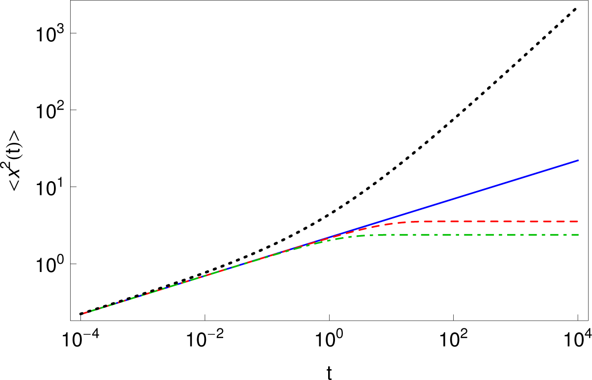
MSD for the fractional diffusion equation (4.6) with α = 1/4 (blue solid line), MSD for the tempered fractional diffusion equation (4.20) with α = 1/4 and b = 0.1 (red dashed line), b = 0.5 (green dot-dashed line). The MSD (4.9) for the bi-fractional diffusion equation in modified form with, a₁ = a₂ = 1/2, α₁ = 1/4 and α₂ = 3/4 is multiplied by factor 2 (black dotted line).

5 Normal versus modified generalized diffusion equation

In our previous work [46] we demonstrated that the CTRW model with waiting time PDF of form

where γ̂(s) is completely monotone and sγ̂(s) is a Bernstein function [49] (or alternatively, sγ̂(s) is a complete Bernstein function), and a Gaussian distribution of jump lengths yields the generalized diffusion equation in normal form

In comparison to the waiting time PDF (3.2) we conclude that there is a connection between both models simply by exchanging γ̂(s) → 1[sη̂(s)]. Thus, if this connection is fulfilled the solutions of both generalized diffusion equations in normal (5.2) and modified form (3.5) will be identical.

Let us illustrate this point. We saw that in the case of η(t) = 1 (η̂(s) = 1/s) we have a Poisson waiting time PDF (4.2) and the classical diffusion equation (4.1). So, if we use that γ̂(s) = 1/[sη̂(s)] = 1, i.e., γ(t) = δ(t), from relations (5.1) and (5.2) we obtain the same results.

Next, the memory kernel η(t) = t^α−1/Γ(α), 0 < α < 1, and η̂(s) = s^−α, corresponds to the M-L waiting time PDF (4.5) and the fractional diffusion equation (4.4). Therefore, by using γ̂(s) = 1/s^1−α, γ(t) = t^−α/Γ(1 − α), the generalized diffusion equation (5.2) becomes the time fractional diffusion equation in the Caputo sense,

which, as we know [46] is an equivalent formulation of the fractional diffusion equation (4.4) as long as the initial values are properly taken into account.

From the previous results [7, 47] we know that the bi-fractional diffusion equations in normal and modified form do not give the same results for the PDF and the MSD. The first one leads to decelerating subdiffusion, and the second one to accelerating subdiffusion. In order to find the equivalent formulation for the bi-fractional diffusion equation in modified form (4.7), we should use γ̂(s) = 1/[s(a₁s^−α₁ + a₂s^−α₂)], 0 < α₁ < α₂ < 1, from where, by inverse Laplace transform, we find that γ(t) is given by

Therefore, the equation in normal form corresponding to (4.7) in modified form is given by

We finally discuss one more example with the tempered memory kernel η(t) = e^−btt^α−1/Γ(α), 0 < α < 1, b > 0, which leads to the tempered fractional diffusion equation (4.18). Setting γ̂(s) = 1/[s(s + b)^−α], (η̂(s) = (s + b)^−α), we find that

and the corresponding diffusion equation in normal form becomes

Conversely, let us consider the memory kernel γ(t) = a₁t^−α₁/Γ(1 − α₁) + a₂t^−α₂/Γ(1 − α₂), 0 < α₁ < α₂ < 1, which leads to the bi-fractional diffusion equation in the normal form,

From the memory kernel we find that η̂(s) = [a₁s^α₁ + a₂s^α₂]⁻¹, i.e.,

Therefore, the equation corresponding to the bi-fractional diffusion equation in normal form turns into the following equation in modified form

In case of a tempered memory kernel γ(t) = e^−btt^−α/Γ(1 α), 0 < α < 1, b > 0, the corresponding equation of the tempered fractional diffusion equation in normal form

is

since

With these examples we show that many different equations with a wide range of memory kernels are special cases of the generalized diffusion equations (3.5) and (5.2).

6 Conclusion

We provided a CTRW model that corresponds to the generalized diffusion equation in modified form. We show that many different generalized derivatives are special cases of the generalized derivative considered in this paper. We also discuss the connection between the generalized diffusion equations in modified and normal form. We show that, for example, the bi-fractional diffusion equation and the tempered fractional diffusion equation in modified form can be represented in normal form by using Mittag-Leffler memory kernels. The need for better fitting of the experimental results [18, 35] requires introducing more flexible theoretical models as those analyzed in this work. Studying of ageing and weak ergodicity breaking [32, 56] often observed in experiments for this more general setting is left for future investigation.

References

[1] J.-P. Bouchaud and A. Georges, Anomalous diffusion in disordered media: Statistical mechanisms, models and physical applications. Phys. Rep. 195 (1990), 127–293.10.1016/0370-1573(90)90099-NSearch in Google Scholar
[2] A. Caspi, R. Granek, and M. Elbaum, Enhanced diffusion in active intracellular transport. Phys. Rev. Lett. 85 (2000), 5655–5658.10.1103/PhysRevLett.85.5655Search in Google Scholar PubMed
[3] A.V. Chechkin, V. Gonchar, R. Gorenflo, N. Korabel, and I.M. Sokolov, Generalized fractional diffusion equations for accelerating subdiffusion and truncated Lévy flights. Phys. Rev. E78 (2008), Art. # 021111.10.1103/PhysRevE.78.021111Search in Google Scholar PubMed
[4] A.V. Chechkin, R. Gorenflo, I.M. Sokolov, Retarding subdiffusion and accelerating superdiffusion governed by distributed-order fractional diffusion equations. Phys. Rev. E, 66 (2002), Art. # 046129.10.1103/PhysRevE.66.046129Search in Google Scholar PubMed
[5] A.V. Chechkin, R. Gorenflo, I.M. Sokolov and V.Yu. Gonchar, Distributed order fractional diffusion equation. Fract. Calc. Appl. Anal. 6, No 3 (2003), 259–279.Search in Google Scholar
[6] A.V. Chechkin, J. Klafter and I.M. Sokolov, Fractional Fokker-Planck equation for ultraslow kinetics. EPL63 (2003), 326–332.10.1209/epl/i2003-00539-0Search in Google Scholar
[7] A. Chechkin, I.M. Sokolov and J. Klafter, Natural and modified forms of distributed order fractional diffusion equations. In: Fractional Dynamics: Recent Advances, World Scientific, Singapore (2011).Search in Google Scholar
[8] A. Erdélyi, W. Magnus, F. Oberhettinger and F.G. Tricomi, Higher Transcedential Functions, Vol. 3. McGraw-Hill, New York (1955).Search in Google Scholar
[9] W. Feller, An Introduction to Probability Theory and Its Applications, Vol. II. Wiley, New York (1968).Search in Google Scholar
[10] K.S. Fa and K.G. Wang, Integrodifferential diffusion equation for continuous-time random walk. Phys. Rev. E81 (2010), Art. # 011126.10.1103/PhysRevE.81.011126Search in Google Scholar PubMed
[11] R. Garra and R. Garrappa, The Prabhakar or three parameter Mittag–Leffler function: Theory and application. Commun. Nonlin. Sci. Numer. Simul. 56 (March 2018), 314–329; 10.1016/j.cnsns.2017.08.018.Search in Google Scholar
[12] R. Garra, R. Gorenflo, F. Polito, and Z. Tomovski, Hilfer-Prabhakar derivatives and some applications. Appl. Math. Comput. 242 (2014), 576–589.10.1016/j.amc.2014.05.129Search in Google Scholar
[13] R. Garrappa, F. Mainardi, and G. Maione, Models of dielectric relaxation based on completely monotone functions. Fract. Calc. Appl. Anal. 19, No 5 (2016) 1105–1160; 10.1515/fca-2016-0060; https://www.degruyter.com/view/j/fca.2016.19.issue-5/issue-files/fca.2016.19.issue-5.xml.Search in Google Scholar
[14] I. Golding and E. C. Cox, Physical nature of bacterial cytoplasm. Phys. Rev. Lett. 96 (2006), Art. # 098102.10.1103/PhysRevLett.96.098102Search in Google Scholar PubMed
[15] H.J. Haubold, A.M. Mathai, and R.K. Saxena, Mittag-Leffler functions and their applications. J. Appl. Math. 2011 (2011), Art. # 298628.10.1155/2011/298628Search in Google Scholar
[16] R. Hilfer, Exact solutions for a class of fractal time random walks. Fractals3 (1995), 211–216.10.1142/S0218348X95000163Search in Google Scholar
[17] R. Hilfer and L. Anton, Fractional master equations and fractal time random walks. Phys. Rev. E51 (1995), Art. # R848.10.1103/PhysRevE.51.R848Search in Google Scholar
[18] F. Höfling and T. Franosch, Anomalous transport in the crowded world of biological cells. Rep. Prog. Phys. 76 (2013), Art. # 046602.10.1088/0034-4885/76/4/046602Search in Google Scholar PubMed
[19] B.D. Hughes, Random Walks and Random Environments, Vol. 1: Random Walks. Clarendon Press, Oxford (1995).Search in Google Scholar
[20] M.C. Jullien, J. Paret, and P. Tabeling, Richardson pair dispersion in two-dimensional turbulence. Phys. Rev. Lett. 82 (1999), 2872–2875.10.1103/PhysRevLett.82.2872Search in Google Scholar
[21] J.-H. Jeon, V. Tejedor, S. Burov, E. Barkai, C. Selhuber-Unkel, K. Berg-Sërensen, L. Oddershede, and R. Metzler, In Vivo Anomalous Diffusion and Weak Ergodicity Breaking of Lipid Granules. Phys. Rev. Lett. 106 (2011), Art. # 048103.Search in Google Scholar
[22] A. Kochubei, General fractional calculus, evolution equations, and renewal processes. Integr. Eq. Operator Theory71 (2011), 583–600.10.1007/s00020-011-1918-8Search in Google Scholar
[23] R. Kutner and J. Masoliver, The continuous time random walk, still trendy: fifty-year history, state of art and outlook. Eur. Phys. J., B90 (2017), Art. # 50.10.1140/epjb/e2016-70578-3Search in Google Scholar
[24] M.A. Lomholt, L. Lizana, R. Metzler, and T. Ambjörnsson, Microscopic origin of the logarithmic time evolution of aging processes in complex systems. Phys. Rev. Lett. 110 (2013), Art. # 208301.10.1103/PhysRevLett.110.208301Search in Google Scholar PubMed
[25] Y. Luchko and R. Gorenflo, An operational method for solving fractional differential equations with the Caputo derivatives. Acta Math. Vietnamica24 (1999), 207–233.Search in Google Scholar
[26] Y. Luchko and M. Yamamoto, General time fractional diffusion equation: some uniqueness and existence results for the initial-boundary-value problems. Fract. Calc. Appl. Anal. 19, No 3 (2016), 676–695; 10.1515/fca-2016-0036; https://www.degruyter.com/view/j/fca.2016.19.issue-3/issue-files/fca.2016.19.issue-3.xml.Search in Google Scholar
[27] E. Lutz, Fractional Langevin equation. Phys. Rev. E64 (2001), Art. # 051106.10.1142/9789814340595_0012Search in Google Scholar
[28] R. Mankin, K. Laas, and A. Sauga, Generalized Langevin equation with multiplicative noise: Temporal behavior of the autocorrelation functions. Phys. Rev. E83 (2011), Art. # 061131.10.1103/PhysRevE.83.061131Search in Google Scholar
[29] F. Mainardi, Fractional Calculus and Waves in Linear Viscoelesticity: An Introduction to Mathematical Models. Imperial College Press, London (2010).10.1142/p614Search in Google Scholar
[30] M.M. Meerschaert, D.A. Benson, H.P. Scheffler, and B. Baeumer, Stochastic solution of space-time fractional diffusion equations. Phys. Rev. E65 (2002), Art. # 041103.10.1103/PhysRevE.65.041103Search in Google Scholar
[31] M.M. Meerschaert and H. P. Scheffler, Stochastic model for ultraslow diffusion. Stochastic Process. Appl. 116 (2006), 1215–1235.10.1016/j.spa.2006.01.006Search in Google Scholar
[32] R. Metzler, J.-H. Jeon, A. G. Cherstvy, and E. Barkai, Anomalous diffusion models and their properties: non-stationarity, non-ergodicity, and ageing at the centenary of single particle tracking. Phys. Chem. Chem. Phys. 16 (2014), Art. # 24128.10.1039/C4CP03465ASearch in Google Scholar
[33] R. Metzler and J. Klafter, The random walk’s guide to anomalous diffusion: A fractional dynamics approach. Phys. Rep. 339 (2000), 1– 77.10.1016/S0370-1573(00)00070-3Search in Google Scholar
[34] E.W. Montroll and G.H. Weiss, Random Walks on Lattices, II. J. Math. Phys. 6 (1965), 167–181.10.1063/1.1704269Search in Google Scholar
[35] K. Nørregaard, R. Metzler, C.M. Ritter, K. Berg-Sørensen, and L.B. Oddershede, Manipulation and motion of organelles and single molecules in living cells. Chem. Rev. 117 (2017), 4342–4375.10.1021/acs.chemrev.6b00638Search in Google Scholar PubMed
[36] M.D. Ortigueira and J.A.T. Machado, What is a fractional derivative? J. Comput. Phys. 293 (2015), 4–13.10.1016/j.jcp.2014.07.019Search in Google Scholar
[37] J. Paneva-Konovska, Convergence of series in three parametric Mittag-Leffler functions. Math. Slovaca64 (2014), 73–84.10.2478/s12175-013-0188-0Search in Google Scholar
[38] J. Paneva-Konovska, From Bessel to Multi-Index Mittag Leffler Functions: Enumerable Families, Series in them and Convergence. World Scientific Publishing, London (2016).10.1142/q0026Search in Google Scholar
[39] J. Paneva-Konovska, Overconvergence of series in generalized Mittag-Leffler functions. Fract. Calc. Appl. Anal. 20, No 2 (2017), 506–520; 10.1515/fca-2017-0026; https://www.degruyter.com/view/j/fca.2017.20.issue-2/issue-files/fca.2017.20.issue-2.xml.Search in Google Scholar
[40] I. Podlubny, Fractional Differential Equations. Academic Press, San Diego (1999).Search in Google Scholar
[41] N. Pottier, Relaxation times distributions for an anomalously diffusing particle. Physica A390 (2011), 2863–2879.10.1016/j.physa.2011.03.029Search in Google Scholar
[42] T.R. Prabhakar, A singular equation with a generalized Mittag-Leffler function in the kernel. Yokohama Math. J. 19 (1971), 7–15.Search in Google Scholar
[43] J.F. Reverey, J.-H. Jeon, H. Bao, M. Leippe, R. Metzler, and C. Selhuber-Unkel, Superdiffusion dominates intracellular particle motion in the supercrowded cytoplasm of pathogenic Acanthamoeba castellanii. Sci. Rep. 5 (2014), Art. # 11690.10.1038/srep11690Search in Google Scholar PubMed PubMed Central
[44] L.F. Richardson, Atmospheric diffusion shown on a distance-neighbour graph. Proc. Roy. Soc. A110 (1926), 709–737.10.1098/rspa.1926.0043Search in Google Scholar
[45] L.P. Sanders, M.A. Lomholt, L. Lizana, K. Fogelmark, R. Metzler, and T. Ambjörnsson, Severe slowing-down and universality of the dynamics in disordered interacting many-body systems: Ageing and ultraslow diffusion. New J. Phys. 16 (2014), Art. # 113050.10.1088/1367-2630/16/11/113050Search in Google Scholar
[46] T. Sandev, A. Chechkin, H. Kantz, and R. Metzler, Diffusion and Fokker-Planck-Smoluchowski equations with generalized memory kernel. Fract. Calc. Appl. Anal. 18, No 4 (2015), 1006–1038; 10.1515/fca-2015-0059; https://www.degruyter.com/view/j/fca.2015.18.issue-4/issue-files/fca.2015.18.issue-4.xml.Search in Google Scholar
[47] T. Sandev, A. Chechkin, N. Korabel, H. Kantz, I.M. Sokolov and R. Metzler, Distributed-order diffusion equations and multifractality: Models and solutions. Phys. Rev. E92 (2015), Art. # 042117.10.1103/PhysRevE.92.042117Search in Google Scholar PubMed
[48] T. Sandev, R. Metzler and Ž. Tomovski, Velocity and displacement correlation functions for fractional generalized Langevin equations. Fract. Calc. Appl. Anal. 15, No 3 (2012), 426–450; 10.2478/s13540-012-0031-2; https://www.degruyter.com/view/j/fca.2012.15.issue-3/issue-files/fca.2012.15.issue-3.xml.Search in Google Scholar
[49] T. Sandev, I.M. Sokolov, R. Metzler, and A. Chechkin, Beyond monofractional kinetics. Chaos Solitons Fractals102 (2017), 210–217.10.1016/j.chaos.2017.05.001Search in Google Scholar
[50] T. Sandev and Z. Tomovski, Langevin equation for a free particle driven by power law type of noises. Phys. Lett. A378 (2014), 1–9.10.1016/j.physleta.2013.10.038Search in Google Scholar
[51] T. Sandev, Z. Tomovski and J.L.A. Dubbeldam, Generalized Langevin equation with a three parameter Mittag-Leffler noise. Physica A390 (2011), 3627–3636.10.1016/j.physa.2011.05.039Search in Google Scholar
[52] H. Scher and M. Lax, Stochastic transport in a disordered solid, I. Theory. Phys. Rev. B7 (1973), Art. # 4491.10.1103/PhysRevB.7.4491Search in Google Scholar
[53] H. Scher, G. Margolin, R. Metzler, J. Klafter and B. Berkowitz, The dynamical foundation of fractal stream chemistry: The origin of extremely long retention times. Geophys. Res. Lett. 29 (2002), Art. # 1061.10.1029/2001GL014123Search in Google Scholar
[54] H. Scher and E.W. Montroll, Anomalous transit-time dispersion in amorphous solids. Phys. Rev. B12 (1975), Art. # 2455.10.1103/PhysRevB.12.2455Search in Google Scholar
[55] R. Schilling, R. Song and Z. Vondracek, Bernstein Functions. De Gruyter, Berlin (2010).10.1515/9783110215311Search in Google Scholar
[56] J.H.P. Schulz, E. Barkai, and R. Metzler, Aging renewal theory and application to random walks. Phys. Rev. X4 (2014), Art. # 011028.10.1103/PhysRevX.4.011028Search in Google Scholar
[57] Ya.G. Sinai, The limiting behavior of a one-dimensional random walk in a random medium. Theory Probab. Appl. 27 (1982), 256–268.10.1007/978-1-4419-6205-8_2Search in Google Scholar
[58] E. Soika, R. Mankin, and J. Priimets, Generalized Langevin equation with multiplicative trichotomous noise. Proc. Estonian Acad. Sci. 61 (2012), 113–127.10.3176/proc.2011.2.04Search in Google Scholar
[59] I.M. Sokolov and J. Klafter, From diffusion to anomalous diffusion: A century after Einstein’s Brownian motion. Chaos15 (2005), Art. # 26103.10.1063/1.1860472Search in Google Scholar PubMed
[60] T.H. Solomon, E.R. Weeks and H.L. Swinney, Observation of anomalous diffusion and Lévy flights in a two-dimensional rotating flow. Phys. Rev. Lett. 71 (1993), Art. # 3975.10.1103/PhysRevLett.71.3975Search in Google Scholar PubMed
[61] A. Stanislavsky and K. Weron, Atypical case of the dielectric relaxation responses and its fractional kinetic equation. Fract. Calc. Appl. Anal. 19, No 1 (2016) 212–228; 10.1515/fca-2016-0012; https://www.degruyter.com/view/j/fca.2016.19.issue-1/issue-files/fca.2016.19.issue-1.xml.Search in Google Scholar
[62] S.M.A. Tabei, S. Burov, H.Y. Kim, A. Kuznetsov, T. Huynh, J. Jureller, L.H. Philipson, A.R. Dinner and N.F. Scherer, Intracellular transport of insulin granules is a subordinated random walk. Proc. Natl. Acad. Sci. USA110 (2013), 4911–4916.10.1073/pnas.1221962110Search in Google Scholar PubMed PubMed Central
[63] V.E. Tarasov, No violation of the Leibniz rule. No fractional derivative. Commun. Nonlin. Sci. Numer. Simul. 18 (2013), 2945–2948.10.1016/j.cnsns.2013.04.001Search in Google Scholar
[64] A.A. Tateishi, E.K. Lenzi, L.R. da Silva, H.V. Ribeiro, S. Picoli Jr. and R.S. Mendes, Different diffusive regimes, generalized Langevin and diffusion equations. Phys. Rev. E85 (2012), Art. # 011147.10.1103/PhysRevE.85.011147Search in Google Scholar PubMed
[65] A.D. Vinãles and M.A. Despόsito, Anomalous diffusion induced by a Mittag-Leffler correlated noise. Phys. Rev. E75 (2007), Art. # 042102.Search in Google Scholar
[66] A.D. Viñales, K.G. Wang, and M.A. Despόsito, Anomalous diffusive behavior of a harmonic oscillator driven by a Mittag-Leffler noise. Phys.Rev. E80 (2009), Art. # 011101.10.1103/PhysRevE.80.011101Search in Google Scholar PubMed
© 2018 Diogenes Co., Sofia
Articles in the same Issue
- Frontmatter
- Editorial Note
- FCAA related news, events and books (FCAA–volume 21–1–2018)