The efficiency of linear electromagnetic vibration-based energy harvester at resistive, capacitive and inductive loads
-
Aboozar Dezhara


Abstract
Energy harvesters and almost all energy generation devices receive the motivation for design from their efficiency and efficiency play an important role in the feasibility and practicability of the design. In this paper, we investigate the efficiency of electromagnetic vibration-based energy harvesters at various electrical loads. In our problem the efficiency depends on excitation frequency, coil and load parameters as well as electromagnetic coupling coefficient. The author first proves that the input power that the harvester receives from its environment at constant base acceleration and constant excitation frequency is always equal to the power that consumes in electrical and mechanical dampers, then the author defines the resonance frequency and plot three efficiency diagrams i.e. plot of efficiency versus (excitation) frequency, plot of maximum efficiency at a constant frequency versus load and in the end plot of the efficiency versus output power at varying load capacitance and resistance. The author observes that maximum efficiency not only does not occur at resonance (i.e. at maximum power) but also is very low (less than 1e−10%) for typical parameters at resonance. Also the maximum efficiency for typical optimum parameters is around 17.45%.
Introduction
Efficiency is a fundamental parameter used to compare all kinds of energy harvesters with various sizes and designs. Usually the main goal of an energy harvesting system is to extract the maximum power from the environment. Almost all the authors have focused their efforts on maximizing the extracted electrical power for linear electromagnetic vibration-based energy harvesters (EVEH) and only a few of them have focused on maximizing efficiency (Almoneef and Ramahi 2015; Ashraf et al. 2013; Bright 2001; Blad and Tolou 2019; Roundy 2005; Smits and Cooney 1991; Wang et al. 1999; Wang and Cross 1998; Zhang et al. 2019). Among these a few, most of them focus on resistive load only. In this paper, we consider inductive and capacitive loads as well. The optimal resistor formula and the numeric optimal capacitor and inductor values that maximize the efficiency have been determined. Here efficiency is defined as the ratio of the electrical power extracted from the load resistor (output power) to the time rate of vibration energy of the environment (input power). Efficiency is considered one variable function of load resistance in resistive load, and is two variables for capacitive and inductive load, respectively. The efficiency is plotted versus excitation frequency at constant optimum coil and load parameters as well as constant electromagnetic coupling coefficient. Then the efficiency and output power is plotted versus load and the author observe that the maximum efficiency dose not occur at resonance frequency in other words load that maximize output power differs with the load that maximize efficiency. The efficiency versus variable load at constant parameters as well as constant resonance frequency is plotted and also efficiency versus excitation frequency at optimum loads is plotted. It should be noted that according the definition of resonance the resistive as well as inductive load dose not lead to a real or true resonance frequency and optimum case at Micro and Nano dimensions except for rare cases (this will be explained later in this paper).
Basic principles of EVEH
In this section we define resonance frequency and calculate the power consumed in the load resistor for three above mentioned loads i.e. resistive, capacitive and inductive loads.
Definition of resonance
The definition of resonance differ from the other mechanical problems because here we seek condition that will maximize the electrical damping term in our problem and this is in contrast to other problems that the damping is a minimum and amplitude should have a maximum value. For resonance (the optimum frequency), the most important following conditions should be satisfied simultaneously:[1]
The result of condition 1 should be absolute maximum point and the result of condition 2 should be local minimum point. The third condition is partial derivative of total stored energy versus time that should be zero i.e. sum of all energy in the capacitors and inductors of electrical equivalent system is constant.
Equivalent circuit of EVEH
Based on the electrical similarity of mechanical systems (Cammarano et al. 2010) we can say:
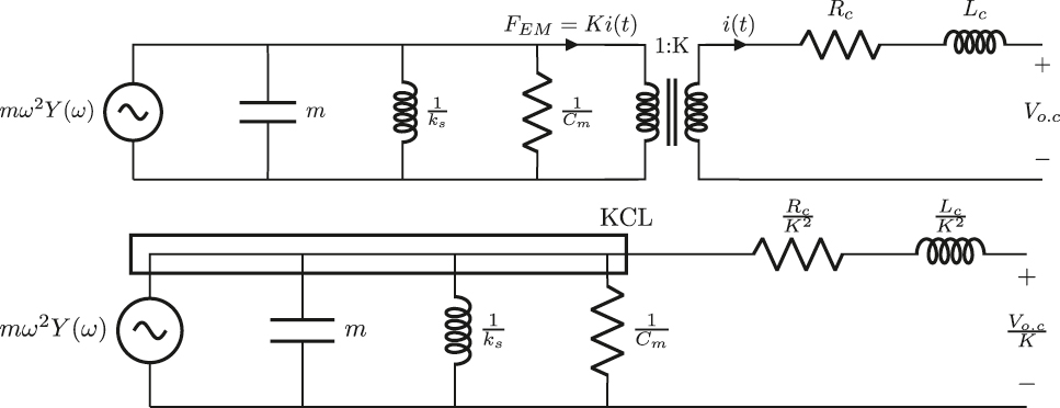
A diagram of the EVEH circuit is shown in Figure 1. FEM is the electrical damping force and
where X′ is the admittance of capacitor and inductor at mechanical side of Figure 2. Based on the Figure 3 we can also calculate short circuit current.
If we substitute equation (10) into (8):
After simplifying we have:

The circuit model of EVEH.
Thévénin circuit for open circuit voltage.

Thévénin circuit of short circuit current.

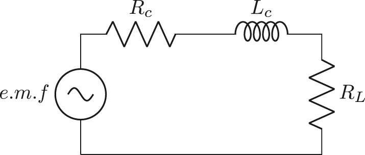
Thévénin equivalent circuit for resistive load.

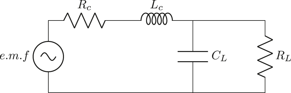
Thévénin equivalent circuit for capacitive load.

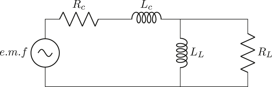
Thévénin equivalent circuit for inductive load.

Electrical side of EVEH for resistive load.
Electrical side of EVEH for capacitive load.
Electrical side of VEH for inductive load.
Electrical side of EVEH for resistive load

EVEH’s electrical side for capacitive loads.

The electrical side of the EVEH for inductive loads.
The condition of maximum power transfer
If the load impedance is equal to the conjugate of Thévénin impedance, then maximum power will be delivered from the source to the load (Cammarano et al. 2010). Note that this is true just for resistive load and in the case of capacitive and inductive loads the derivative of real power consumed in the load resistor in terms of load resistor and capacitor should be equaled to zero for obtaining the optimum load and rendering reactive part of Thévénin reactance to zero.
Resistive load
Based on the Figure 4 we have:
Capacitive load
Based on the Figure 5, if you calculate the power consumed in the load resistor and equal the derivative of this power with respect to
Putting the relation of (18) into (17), the result is:
These equations are the optimum load formula for capacitive loads. Note that the optimum resistor is not equal to the Thévénin resistor.
Inductive load
Based on the Figure 6 and similar to the capacitive load we have:
putting the relation of (21) into (20), the result is:
These equations are the optimum load formulas for inductive load. Note that the optimum resistor is exactly the same as the case of capacitive load resistor.
The input power duo to vibration of environment
In this subsection the input power to the EVEH will be calculated and the author shows that this power is equal to power that consumes in the electrical and mechanical dampers. Consider the equivalent circuit of EVEH (Figure 1), the input power is equal to the power that is generated in the current source of the circuit.
where
Based on the differential equation governing the problem in frequency domain we have:
Now if the resonance condition (relation 3) is applied to the transfer function (Dezhara 2022) we can simplify the above equation.
If we put the equation (27) into equation (26) we have:
After simplifying equation (28):
The relation (29) tell us that the input power at resonance is equals to power that consumed in the mechanical and electrical dampers.
The specified load in various modes
Here the author determines the modes of load that should be applied in various condition in Table 1. It should be noted that the first case i.e. when excitation frequency is less that mechanical resonance frequency and Thévénin reactance (equation (14)) is positive, is the most popular mode and other cases are very rare at least in micro dimension. Based on the Thévénin reactance, when the excitation is less than mechanical resonance frequency, the Thévénin reactance has never a negative value and is always positive. So the case of
The loads that should be applied in various conditions.
| Frequency | Thévénin reactance | Applied load |
|---|---|---|
|
|
|
|
|
|
|
|
|
|
|
|
Resistive load calculations
In the Figure 7, if we designate the load voltage
where
RMS Power for resistive load
The power is the time derivative work of the electric damping force
We can calculate the power based on the generated electrical current. Inputting equation (33) into equation (35):
By putting equations (32) into (36), we can derive the power formula:
Based on the simplified equation above:
The real part of equation (41) corresponds to the electrical damping, which is a factor that affects the mechanical damping coefficient. The imaginary part of electrical coefficient i.e. imaginary part of equation (41) is called lock coefficient (Dezhara 2022). Reactive power may also be generated by the passive components of the circuit such as mass and spring. The reactive energy always flows from the electrical part, i.e. load capacitor and coil inductor, to the mechanical part, i.e. mass and spring. It’s easy to conclude that the real part of equation (39) is energy generated in a coil and a load resistors, the imaginary part refers to the reactive energy generated in the coil’s inductor. The resistor
Capacitive load calculations
Based on the Figure 8, we can write the circuit equation of energy harvester with capacitive load as follows:
where
Now we should someway obtain the
If we put equation (47) into equation (49) and solve for
If we put equation (51) into equation (47) we will have:
RMS Power for capacitive load
Knowing the coil current we now can derive power formula versus frequency based on the definition of power (equation (34)):
In order to distinguish real power generated in
The real power is the sum of power that is generated in the coil and in the load. We can distinguish between these two powers, i.e.
Subtracting equation (56) from equation (54) we find the power consumed by the resistor of the load (i.e.
The frequency-response plot is the plot of
we would like to conform equation (53) into standard form:
The electrical damping coefficient of EVEH can be calculated by simplifying the equation of (54).
The imaginary part of complex damping based on simplification of equation of (58) is:
Inductive load calculations
Based on the Figure 9 we have:
When we put the equation (62) into frequency domain, we get the following:
We solve for
RMS Power for inductive load
Here is the real part of the equation:
As a result of subtracting equation (74) from equation (71):
Efficiency
In this section the formulas for efficiency at resistive and capacitive and inductive load are derived. It should be noted that in the case of capacitive as well as inductive loads the efficiency is usually function of two variables the resistance and capacitance or inductance.
where:
E: kinetic energy of moving magnet (mass)
U: potential energy of spring
Wd: dissipated energy in mechanical damper
We: dissipated energy by electrical damping mechanism.
Resistive load
Here the typical values of efficiency is investigated note that these values are not true values.As noted previously, the time rate of the sum of kinetic and potential energies is zero as the vibration of the EVEH is forced and the sum of potential energy of the spring and kinetic energy of mass is constant, resulting in a zero time derivative of the energy. For resistive loads, based on the Figure 10 the output power consumed in the load resistor is:
from the above equation:
The
It is shown in equation (85) that efficiency varies with load resistor i.e.
As a result, this resistor will maximize the efficiency of the resistive load EVEH, note that this resistance is not equal to the resistance that maximizes the power extracted by EVEH.
Capacitive load
The output power consumed in the resistor of Figure 11 is:
according to above equation:
According to equation (4), the input power is:
MATLAB software can maximize this function which is a two-variable function of
Inductive load
The out power that consumes in resistor of Figure 12 is (Dezhara 2022):
After simplifying of
MATLAB can also maximize the above equation, which is a two variable function of
Numerical example
In this section for resistive load case we just plot the efficiency function based on the typical data with respect to load because in these case the resonance that we have defined in Section 2.1 dose not lead to a real answer (the case of
Typical numerical data for resistive load.
| 1 |
|
Coil inductance | 0.2 | mH |
| 2 |
|
Coil resistance | 3 |
|
| 3 |
|
Electromagnetic coupling coefficient | 5 |
|
| 4 |
|
Excitation frequency | 100 |
|
| 5 |
|
Mechanical damping coefficient | 0.05 |
|
Resistive load
Using the Figures 13 and 14 we can get these results:

Efficiency plot at constant K,

Efficiency plot at constant
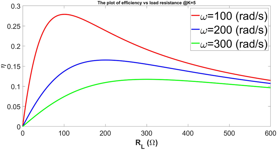
Efficiency plot at constant K,
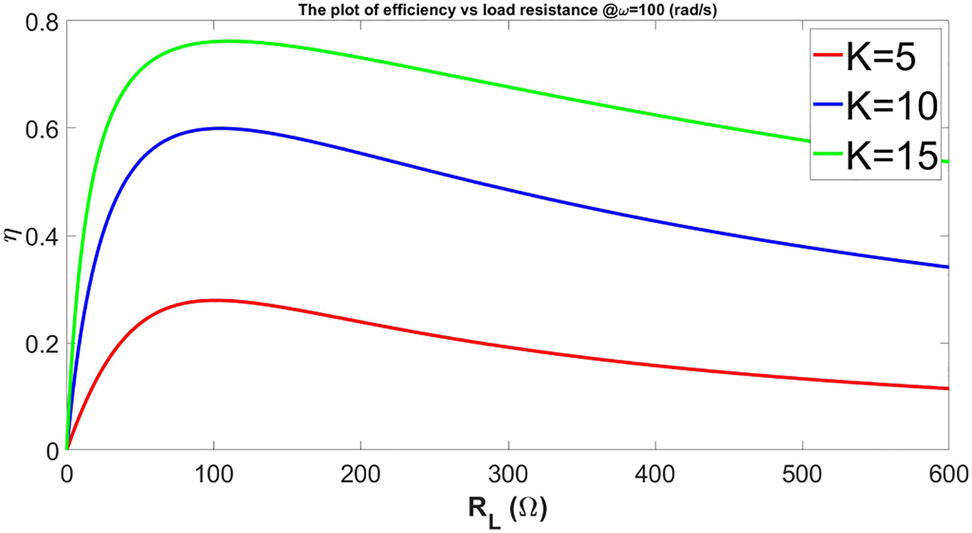
Efficiency plot at constant
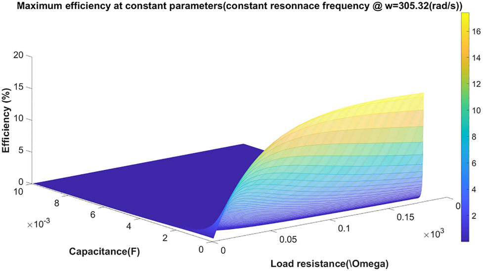
Maximum efficiency versus load.

Maximum power versus load.

Efficiency versus excitation frequency for capacitive load.

Efficiency at constant resistance but varying load capacitance versus output power.
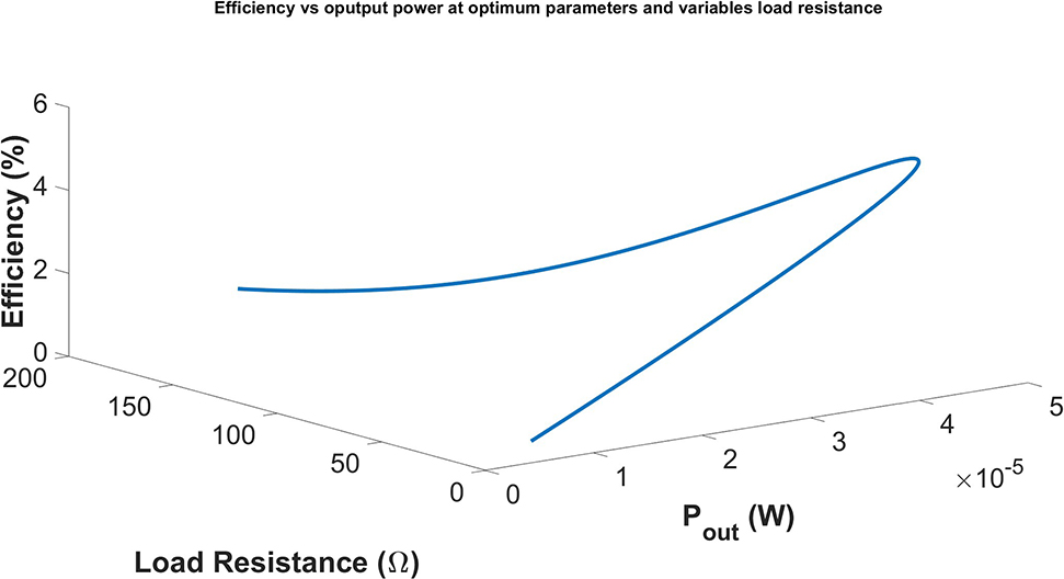
Efficiency at constant capacitance but varying load resistance versus output power.
Note that according to Figure 13 for
Capacitive load
Generally in the case of capacitive load (at high mechanical resonance frequency which is the case for micro or nano dimension) the definition of resonance leads to a numeric answer i.e. optimum load and coil parameters and optimum resonance frequency at assumed constant mechanical parameters.[3]
Note that the data of Table 3 is derived based on the definition of resonance and constant mechanical parameters of
Optimum numerical data for capacitive load.
|
|
Resonance frequency | 305.32 |
|
|
|
Coil inductance | 30.85 |
|
|
|
Coil resistance | 99.43 |
|
|
|
Load resistance | 103 |
|
|
|
Load capacitance | 3.1 |
|
|
|
Electromagnetic coupling coefficient | 5.6 |
|
|
|
Mechanical resonance frequency | 387.9 |
|
|
|
Mechanical damping coefficient | 0.31 |
|
|
|
Base acceleration | 1.02 g |
|
Based on the MATLAB calculations the maximum efficiency occurs at
Based on the MATLAB calculations the maximum power occurs at
Note that based on the Figure 19 the value of efficiency at resonance
Note that based on the projection of plots of Figure 20 and Figure 21 efficiency has approximately linear relationship with the output power up to some limits which is less than maximum extracted power i.e.
Conclusions
Based on the resonance definition and numerical results we conclude that the resonance frequency for resistive and inductive loads does not lead to a real answers. Nevertheless we plot the efficiency versus resistive load for typical numeric parameters. We also conclude that the loads that maximize the efficiency differ from the loads that maximize the power, in other words efficiency at maximum power differs from the maximum efficiency. And at mechanical resonance frequency, the efficiency will decrease considerably. Our example shows that the typical maximum efficiency of EVEH for optimum parameters is around 17.45% and this is a low value. Note that with increasing output power the efficiency is also increase but not up to resonance i.e. at some power that considerably less that maximum extracted power.
-
Author contributions: The author has accepted responsibility for the entire content of this submitted manuscript and approved submission.
-
Research funding: None declared.
-
Conflict of interest statement: The author declares no conflicts of interest regarding this article.
References
Almoneef, T. S., and O. M. Ramahi. 2015. “Metamaterial Electromagnetic Energy Harvester with Near Unity Efficiency.” Applied Physics Letters 106 (15): 153902, https://doi.org/10.1063/1.4916232.Search in Google Scholar
Ashraf, K., M. H. M. Khir, J. O. Dennis, and Z. Baharudin. 2013. “Improved Energy Harvesting from Low Frequency Vibrations by Resonance Amplification at Multiple Frequencies.” Sensors and Actuators A: Physical 195: 123–32, https://doi.org/10.1016/j.sna.2013.03.026.Search in Google Scholar
Bright, C. 2001. Energy coupling and efficiency. Sensors 18 (6): 76+78–81.Search in Google Scholar
Blad, T. W. A., and N. Tolou. 2019. “On the Efficiency of Energy Harvesters: A Classification of Dynamics in Miniaturized Generators under Low-Frequency Excitation.” Journal of Intelligent Material Systems and Structures 30 (16): 2436–46, https://doi.org/10.1177/1045389x19862621.Search in Google Scholar
Cammarano, A., S. G. Burrow, D. Barton, A. Carrella, and L. Clare. 2010. “Tuning a Resonant Energy Harvester Using a Generalized Electrical Load.” Smart Materials and Structures 19: 055003, https://doi.org/10.1088/0964-1726/19/5/055003.Search in Google Scholar
Dezhara, A. 2022. “Frequency Response Locking of Electromagnetic Vibration-Based Energy Harvesters Using a Switch with Tuned Duty Cycle.” Energy Harvesting and Systems 9 (1): i–iii, https://doi.org/10.1515/ehs-2022-frontmatter1.Search in Google Scholar
Roundy, S. 2005. “On the Effectiveness of Vibration-Based Energy Harvesting.” Journal of Intelligent Material Systems and Structures 16: 809–23, https://doi.org/10.1177/1045389x05054042.Search in Google Scholar
Smits, J. G., and T. K. Cooney. 1991. “The Effectiveness of a Piezoelectric Bimorph Actuator to Perform Mechanical Work under Various Constant Loading Conditions.” Ferroelectrics 119 (1): 89–105, https://doi.org/10.1080/00150199108223329.Search in Google Scholar
Wang, Q. -M., X. -H. Du, B. Xu, and L. E. Cross. 1999. “Electromechanical Coupling and Output Efficiency of Piezoelectric Bending Actuators.” IEEE Transactions on Ultrasonics, Ferroelectrics, and Frequency Control 46 (3): 638–46, https://doi.org/10.1109/58.764850.Search in Google Scholar PubMed
Wang, Q. -M., and L. E. Cross. 1998. “Performance Analysis of Piezoelectric Cantilever Bending Actuators.” Ferroelectrics 215 (1): 187–213, https://doi.org/10.1080/00150199808229562.Search in Google Scholar
Zhang, L. B., H. L. Dai, Y. W. Yang, and L. Wang. 2019. “Design of High-Efficiency Electromagnetic Energy Harvester Based on a Rolling Magnet.” Energy Conversion and Management 185: 202–10, https://doi.org/10.1016/j.enconman.2019.01.089.Search in Google Scholar
© 2022 Walter de Gruyter GmbH, Berlin/Boston
Articles in the same Issue
- Frontmatter
- Review
- A comprehensive review on electric vehicles: charging and control techniques, electric vehicle-grid integration
- Research Articles
- Evaluation of parameters influencing the performance of photovoltaic-thermoelectric (PV-TE) hybrid system
- Dispatchable power supply from beam down solar point concentrator coupled to thermal energy storage and a Stirling engine
- Modelling, design and parametric analysis of a levitation based energy harvester
- Performance optimization of flywheel using experimental design approach
- Assessment and optimization of photovoltaic systems at the University Ibn Tofail according to the new law on renewable energy in Morocco using HOMER Pro
- Optimizing hybrid power system at highest sustainability
- Preparation of Na2HPO4⋅12H2O-based composite PCM and its application in air insulated box
- The efficiency of linear electromagnetic vibration-based energy harvester at resistive, capacitive and inductive loads
- A numerical investigation of optimum angles for solar energy receivers in the eastern part of Algeria
- Experimental investigation of soiling effects on the photovoltaic modules energy generation
- Frequency domain analysis of a piezoelectric energy harvester with impedance matching network