Investigation of aerodynamic interaction between the balloon and the ducted wind turbine in airborne configuration

Naveen Prakash Noronha; Krishna Munishamaih

doi:10.1515/ehs-2021-0067

40% Rabatt

auf Fachbücher bei De Gruyter Brill *

Artikel Öffentlich zugänglich

Investigation of aerodynamic interaction between the balloon and the ducted wind turbine in airborne configuration

Naveen Prakash Noronha und Krishna Munishamaih

Veröffentlicht/Copyright: 3. Januar 2022

Veröffentlicht von

Veröffentlichen auch Sie bei De Gruyter Brill

Manuskript einreichen Informationen für Autor*innen

Aus der Zeitschrift Energy Harvesting and Systems Band 9 Heft 1

Abstract

An aerodynamic analysis is presented in the current work, which estimates the separation distance between the balloon and the turbine in an airborne wind energy system (AWES). The stability of the structure of AWES depends on the aerodynamic interaction between the turbine and the balloon. A minimum gap must be maintained between the balloon and the wind turbine to reduce the interaction between the balloon and the turbine assembly. Three cases of AWES have been studied with a separation gap of 5 m, 10 m, and 16 m to estimate the minimum distance of separation between the balloon and the turbine. The aerodynamic interaction details suggest that a minimum distance of 13 m needs to be maintained between the turbine and the balloon to avoid the interaction between the balloon and turbine. Steady-state simulations of the rotor are run for various wind conditions to evaluate the efficiency of the duct-mounted configuration. The ducted turbine configuration saw a 7.4% increase in torque than the inducted turbine for a wind speed of 5 m s⁻¹. A torque increase of 17.85% was observed when the separation distance was increased to 16 m from earlier 10 m.

Keywords: airborne wind energy (AWE); optimization; separation gap; small wind turbine

Introduction

Airborne wind energy (AWE) is attracting many researchers and companies due to its newfound relevance. AWE harvests higher altitude wind energy by using multiple methods. AWE’s uniqueness is the accessibility to the high altitude calm streamlined winds available throughout the year (Aglietti et al. 2009; Roberts et al. 2007; Saeed and Kim 2017). AWE is the technology to extract wind energy at higher altitudes, i.e., above 250 m, while the traditional land-based wind turbines operate at about 125–150 m (Archer and Caldeira 2009). The airborne technology concept is not novel; however, the idea has recently gained momentum due to renewed interest in alternative energies. AWE has several other benefits, the most notable of which is the low land area requirement for the installation. The most promising technology among the AWE is the lighter than air system (Chandrasekaran 2020; Vermillion, Glass, and Rein 2013).

Different people and agencies have tried different methods to harness high altitude wind energy to maximize energy generation at the load center.

Buoyant airborne turbine (BAT) is an upcoming research area attracting many researchers among all airborne concepts. BAT system can have many variants based on the design. The BAT system discussed in the present work consists of a wind turbine floating in the air with a helium-filled balloon. Since the entire system is lighter than air, the BAT system is controlled from the Earth through tethers. The balloon maintains the bouncy required to keep the system afloat, whereas the duct provides the system’s orientation in the wind direction. This kind of system efficiently extracts power until 600 m above the ground level; however, momentary air gusts produce large displacements (Ali and Kim 2021; Fagiano, Milanese, and Piga 2010; Reggio, Villalpando, and Ilinca 2011; Sarathkumar Sebastin 2019). The sturdy design of AWS needs a detailed study of the forces exerting on the BAT system. However, the experimental investigations to determine the magnitude and direction of unbalanced forces are virtually impracticable.

As a complex geometry, the BAT system’s interaction with the frequent varying wind speeds is highly complex, consisting of turbulence and high wind shear (Reggio, Villalpando, and Ilinca 2011; Wang 2012). Numerical techniques are used to predict the steady and unsteady flow aerodynamic characteristics of BAT. It is a well-known fact that the experimental methods are capital intensive and require a long time to achieve the desired results. On the other hand, affordable high-end computational facilities and reliable computational methods make the aerodynamic analysis feasible.

The performance of an airborne wind turbine in a shell configuration is investigated for various turbine positions along the axis of the shell. Unsteady aerodynamic simulations have been performed for each turbine position to determine the optimum axial position. To capture the effect of axial position on turbine performance, a minimum of one complete rotation of the turbine is performed. On a scaled model of the NREL-IV rotor, the researchers investigated five axial locations and different wind speeds (7–20 ms⁻¹). The impact of turbine position on the performance of turbine blades, shell body, and turbine performance was also investigated (Saleem and Kim 2011).

In this work, researchers have optimized the airborne wind turbine shell design using a genetic algorithm. Though the turbine is designed by implementing BEM theory through MAT LAB, the optimization of the shell design is significant to maximize the turbine’s performance. The turbine behaves differently when it is open to the atmosphere; however, when the turbine is in a shelled configuration, the performance of the turbine varies. So, an optimum size and shape of the shell are very much required for maximum power production. To address this challenge, researchers studied the influence of the shell shape, turbine position, and shell cross-section on a reference shell configuration based on NACA – 9415 configurations. The aerodynamic investigation is carried out at the height of 400 m above sea level, and wind turbine performance coefficients such as shell thrust coefficient, shell back pressure coefficient, and turbine power coefficient were tested (Saleem and Kim 2020).

The literature mentions many such numerical studies carried out in the domain of wind turbine analysis. The BAT analysis can also be considered as a subcategory of ducted wind turbines; however, the latter is lifted to higher altitudes (Bontempo and Manna 2016; Hu and Cheng 2008; Vinit 2016; Werle and Presz 2008; Zefreh 2016).

An extensive review of the literature related to different numerical methods used to analyze ducted wind turbines is discussed below. Bontempo and Manna (2013) carried out the analysis using the Computational Fluid Dynamics (CFD) technique (Torresi et al. 2016), and the results were compared with the nonlinear as well as semi-analytical actuator disc method (Bontempo and Manna 2014). Upon comparison, they found an excellent correlation between the two methods. Van Bussel (2007), through his newly developed momentum theory, showed that Ducted Wind Turbine (DWT’s) performance could be improved by reducing the backpressure behind the turbine, which depends on the area ratio of the nozzle exit.

Vaz and Wood (2016) proposed another attempt to improve the DWT performance through their model, an enhanced version of blade momentum theory. In their work, they obtained improvements in the twist and chord length of the blade. Bontempo and Manna (2020) analyzed DWT using both nonlinear semi-analytical actuator disc theory and momentum theory. They found the earlier method helpful because it considers divergence and slipstream rotation during the analysis. Politis and Koras (1995) proposed a unique method called the lifting line method for rotor modeling and the lifting surface method for duct modeling. However, in CFD techniques, the entire geometry is divided into small volumes to calculate stress and strain at various geometry parts; this process is called the computational domain’s discretization. Upon discretization, Navier–Stokes equations are used to determine the changes happening in the flow through the principles of conservation of mass, momentum, and energy. The other advantages of CFD methods are the flexibility and accuracy with which the unsteady aerodynamics (Cai et al. 2016), wake effects (Ghasemian and Nejat 2016), and the boundary layer transition effects (Guntur et al. 2016) can be predicted.

This manuscript focuses on the steady aerodynamic prediction of the ducted micro horizontal axis wind turbine (HAWT) in an airborne configuration. The analysis is carried out under varying wind conditions by commercial CFD kit ANSY-Fluent 2020R2. Although several researchers have investigated the aerodynamic performance of the HAWT, the aerodynamic predictions for a turbine at a higher altitude in airborne configuration have never been computed before to the best of the author’s understanding. In addition, aerodynamic analysis for predicting an optimum gap between the balloon and the turbine assembly is not yet attempted. Thus, current research involves the aerodynamic investigation of the airborne ducted wind turbine. The rotor selection for the study was based on the author’s published work (Noronha and Krishna 2020). The numerical research was carried out to understand the impact of high altitude and a duct casing on the wind turbine aerodynamic efficiency with different wind speeds. The findings of the present work will help to optimize the balloon-assisted BATs.

Computational model

A well-known commercial CFD package ANSYS-FLUENT 2020 R2 is used to compute the flow field in the present work. Since the flow field is considered turbulent and compressible, the Reynolds averaged Navier–Stokes equations (RANS) (Patankar 1980; Versteeg and Malaskekera 2007) with no source term are used. The RANS equations are incomplete without the turbulence model, so the turbulence model is inevitable. Based on the computational capabilities, the turbulence model is chosen. The data regarding the boundary layer, pressure drops, and flow properties are essential for accurate aerodynamic predictions. As per the literature, many researchers (Liu and Yoshida 2015; Tavares Dias Do Rio Vaz et al. 2014; van Bussel 2007) have adopted Menter (2012) developed a shear stress transport (SST) turbulence model for better accuracy and details for wind turbine aerodynamics. The selection of a computational model also depends on the computational facilities available. One of the most sought-after two-equations K-ω SST turbulence model is used for the present analysis.

Methodology

Numerical domain specifications

A finite region in space around the turbine is called a computational domain in CFD computations. In the present analysis, a cylindrical domain of diameter 20D, upwind length of 15D, and downwind length of 35D is considered to facilitate differential discretization, as shown in Figure 1. The finer discretization of the computational domain provides good results. However, the computational facilities restrict the element size. The best practice is to coarsen the mesh size away from the model while keeping the finer mesh in the vicinity. This kind of mesh is obtained by tuning proximity and curvature setting in the Ansys mesh feature. The complete design procedure of the turbine used in the present work is discussed in the author’s other publication (Noronha and Krishna 2020). The shell design used in the analysis is referred to from the reference (Roshan, Alimirzazadeh, and Rad 2015). The domain dimensions, upwind and downwind lengths, are decided based on the best practices presented in reference (Saeed and Kim 2016).

Figure 1:

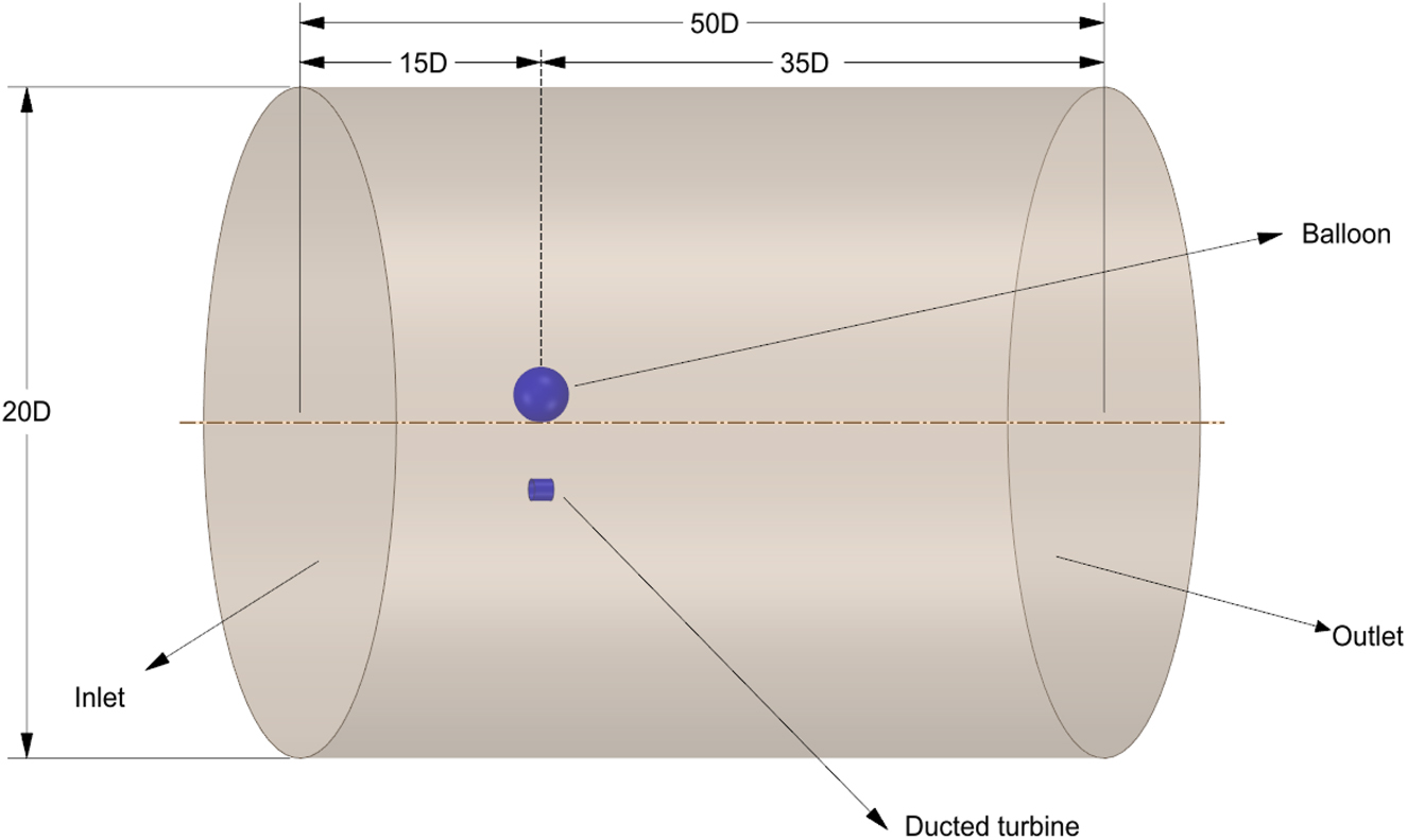
Computational domain specifications.

Figure 1 shows the computational domain specifications used in the present aerodynamic analysis, and wherein D is the diameter of the turbine. The diameter of the turbine is used as a reference in designing and positioning the turbine and balloon.

As shown in Figure 2, a duct of diameter 4 m is considered by providing a gap of 0.5 m between the duct and the turbine, making the duct diameter approximately 1.3D. Figure 3 shows the relative dimensions of the duct as well as the balloon. The balloon dimensions are approximately 3.3D, calculated based on the mass of the turbine assembly and the lifting capacity of helium gas.

Figure 2:

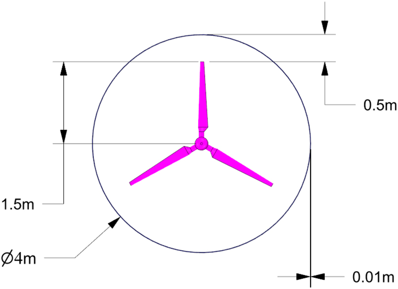
Ducted turbine specifications.

Figure 3:

Airborne turbine arrangement dimensions.

CFD analysis and boundary conditions

In the present work, aerodynamic analysis has been carried out to understand the interaction between the balloon and a turbine assembly in an airborne environment. The turbulence factor is assumed considering the actual nature of the atmospheric conditions. Since the present work is carried out in a low wind speed area, an average wind speed of 5 m s⁻¹ is considered. The height of the airborne wind turbine was fixed at 250 m from the ground level. The atmospheric conditions at higher altitudes vary, and the same can be calculated using Equations (1)–(3).

(1)T=To−6.5 h(m)100

(2)P=PO(1−0.0065 h(m)To)5.2561

(3)ρ=pRT

In the above expressions, T is temperature, p is pressure, and ρ is the density of the air at a higher altitude. Whereas, T_o is the temperature, p_o is the pressure, and ρ_o is the density of the air at ground or sea level. The expression for the velocity variation with the height is found in the reference (Cai et al. 2016).

The pressure boundary condition is applied to the outlet, and the wall boundary condition with the no-slip condition is applied to the far-field, balloon, duct, and turbine surface. The influence of the computational domain boundaries on the results has to be avoided to get error-free results.

Mesh

Discretization is crucial in getting accurate aerodynamic results. Generating a high-quality grid is not difficult; however, obtaining a precise mesh for a complicated geometry such as a wind turbine is quite challenging (El Mouhsine et al. 2018). Figure 4 shows the mesh details of different parts of the wind turbine. The presence of small features in the model leads to skewness in the mesh. A simplified model with little sharp edges and corners needs to be prepared for a better-quality mesh. The mesh near the model needs to be small enough to capture the aerodynamic changes happening near the surface of the boundary. This small length facilitates capturing the boundary phenomena, and this height is called the y⁺ value (Du and Selig 2000).

Figure 4:

Meshing details of the domain and airborne wind energy system (AWES) assembly.

The y⁺ is a non-dimensional length of the first grid layer from the wall. This value is very significant since it captures the typical flow pattern near the wall. So, the first calculation of the flow properties depends on this layer and hence this value.

The y⁺ value is applicable in determining the boundary layer turbulence and depends on the Reynolds number (Re). For higher Re, a lower value of the y⁺ is considered. Generally, the lowest y⁺ value is desirable for better results as the global mesh resolution parameters depend on the near-wall mesh and the Re. The lowest value of y⁺ is also desirable, wherein wall-bounded effects such as aerodynamic drag, heat transfer, and pressure drop are significant. A low Re numbered turbulence model such as the SST model is used to obtain a better value for y⁺ (Mueller 2016).

The y⁺ value is calculated from Equation (4)

(4)y+=ρ.UT.Δy1/μ

wherein U_T is the frictional velocity and is defined as:

UT=τwρ

where τ_w is the shear stress and is defined as:

τw=1/2.Cf.ρ.U2

C _f is the skin friction coefficient shown in Table 1 as a Re function in the above expression.

Table 1:

Skin friction coefficients for internal and external flows.

Flow type	Empirical Estimate
Internal flows	C _f = 0.079. Re^−0.25
External flows	C _f = 0.058. Re^−0.2

The italic values 0.079 and 0.058 are the constants obtained by substituting suitable values for the parameters in the internal and external turbulent flows.

For the present analysis, tetrahedral unstructured mesh topology is obtained by employing the commercial ANSYS – Workbench meshing software.

Mesh independence study

The mesh dependency study was carried out using three different quality meshes Q1, Q2, and Q3. The details of each of the three meshes are provided in Table 2. Though the accuracy of final results depends on the mesh size, a large computational volume requires sophisticated computational facilities (Chowdhury, Akimoto, and Hara 2016).

Table 2:

Mesh details in the computational domain for the numerical study.

Mesh	Total number of nodes	The maximum value of y⁺	CPU time for operation in seconds
Q1	1,643,563	0.2	180
Q2	2,015,626	0.2	250
Q3	3,567,432	0.2	320

The outer domain element size was kept constant; however, proximity and curvature settings were varied to obtain a better mesh quality near the turbine surface. The inflation layers were increased from 5 to 10 by continuously lowering the growth ratio from 1.2 to 1. Through these modifications, mesh independent results were obtained, and the same is presented in Figure 5.

Figure 5:

Pressure variation data for different mesh qualities.

The results presented in Figure 5 show that the maximum difference between the values obtained from meshes of Q2 and Q3 is below 1%. Also, the difference in computational time and space used in both cases is minuscule. Hence mesh of Q2 is chosen for the further computational analysis presented in the present work.

Results and discussion

Aerodynamics of airborne system

Wind turbines operate in the atmospheric boundary sheet, the lowest layer of the atmosphere, called a planetary boundary layer (PBL). Most turbines used to operate in the PBL until recently. This lowest layer of the atmosphere where most turbulence and surface frictional drag are involved is called a surface layer (SL). The SL contains most of the variations in the wind speed and turbulence mixing due to the significant variation of the temperature gradient between day and night. Due to this rigorous mixing of the cold and warm air, huge eddies form. These eddies create a buoyant force and result in the air’s vertical movement with a constant phase until the SL extends.

The height of the SL is usually less during the night due to the absence of higher temperature gradients. This is the reason why the winds above SL have higher velocities than the air in the SL.

The winds above SL are decoupled from the chaos in the SL and have free flow without any hindrance. Consequently, vertical heat and momentum transport (fluxes) are almost constant as height is increased.

The SL is not always stable and static, and its condition depends on the winds at higher altitudes. As the winds at higher altitudes increase, the SL becomes less stable, and its thickness varies. That is the very reason behind increasing the height of the wind turbine.

If the rotor reaches beyond the SL, the streamlined air present over the threshold limit certainly facilitates continuous, uninterrupted power generation. Hence, the present work focuses on capitalizing on the streamlined air present at higher altitudes.

Pressure distribution in the separation gap

The idea of a high altitude floating wind turbine is difficult to realize without a safe floating carrier, in this case, a balloon. The balloon holds the turbine afloat at a high altitude. The duct ensures that it retains its constant wind-facing orientation for stable operation under varying wind speed and direction, such as wind gusts.

The current section describes the effect of change in the separation gap on the aerodynamic forces encountered by the duct, which can help improve the design of AWES. The AWES is subjected to varying forces due to the differential air velocities at higher altitudes.

Also, the relative motion between the balloon and the turbine creates additional movement in the system. Hence, to reduce the turbine’s performance degradation due to the balloon’s presence, a suitable distance needs to be maintained between the balloon and the turbine.

In the present work, numerical analysis is carried out to recognize the effect of balloon turbulence on the turbine’s performance. The present work also aims to determine the minimum distance between the balloon and the wind turbine assembly to avoid turbulence in the air near the turbine.

Figure 6(a)–(c) show the pressure distribution at 5 m, 10 m, and 16 m gap, respectively. Figure 6(a) reveals the overlapping of the balloon turbulence on the turbine. This kind of interaction causes turbulence in the wind turbine and hence reduces the performance of the turbine. The effect of the balloon turbulence on the turbine torque is discussed in the next section. Figure 6(b) shows the pressure distribution around the balloon when the separation distance between the balloon and the turbine is 10 m.

Figure 6:

Pressure contours for (a) 5 m, (b) 10 m, and (c) 16 m distance of separation.

The turbine is seen influenced by the turbulence created by the turbine. So, from the above two cases, it is evident that the distance of separation between the turbine and balloon should be more than 10 m.

The studies were furthered by increasing the distance of separation to 16 m. Figure 6(c) shows a clear separation between the balloon pressure zone and the turbine. Wherein two pressure zones are distinctly separate, indicating the noninterference of the balloon turbulence on the turbine.

Figure 7 shows the pressure probes arranged between the separation gap to measure the change in pressure at equal distances. For the sake of investigation, the turbine and the balloon are considered stationary.

Figure 7:

Pressure probes between the balloon and turbine gap.

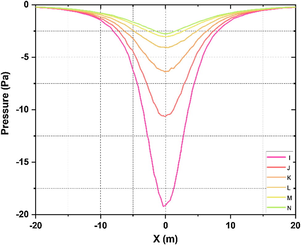
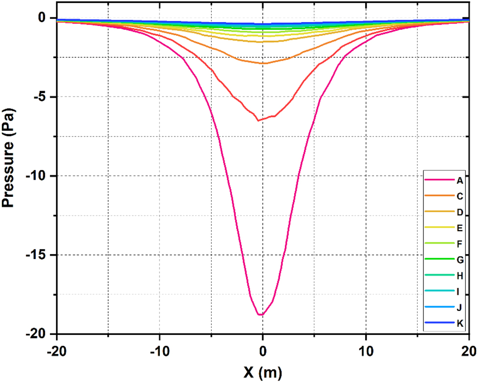
Figure 8 shows the pressure variation between the 5 m separation gap. The pressure probes I–N measure pressure from the balloon end towards the turbine end. Variation of pressure can be seen at every level in decreasing intensity. From the depression in the pressure plots, it can be concluded that there is an influence of balloon pressure near the turbine, and hence the performance of the turbine gets effected. To avoid the influence of balloon pressure, the separation gap was increased to 10 m, and the observations are presented in Figure 9. In the 10 m separation case, the pressure variation is damping as the distance of separation increases. Pressure probe D is arranged very close to the balloon, and every other probe is at a distance of 1 m apart. So from Figure 9, it can be summarized that the pressure probe N, which is at 10 m away from the balloon, still carries the influence of balloon pressure. So to determine the actual distance of separation with no influence of balloon pressure, the distance of separation was increased to 16 m. Figure 10 shows the 16 m separation case wherein the pressure probes are shown till the 13 m gap. The pressure curve N, which indicates the pressure at a distance of 13 m from the balloon, shows almost nil deflection, proving the no influence of balloon pressure. In all the above cases, the operating variables were kept constant except for separation distance.

Figure 8:

Pressure distribution between 5 m gap.

Figure 9:

Pressure distribution between 10 m gap.

Figure 10:

Pressure distribution between 16 m gap.

So from the above analysis, it can be concluded that 13 m could be considered the minimum distance of separation that needs to be maintained between the balloon and the turbine to avoid pressure interference.

Figure 11 shows the comparison of pressure distribution in all three cases. The measurements were taken from the turbine hub, and hence 2 m in the y-direction is near the wind turbine duct. The 16 m gap pressure curve flattens at around 13 m height to indicate almost zero pressure at that distance.

Figure 11:

Pressure distribution between the gap.

Aerodynamics of the duct

The turbine with a duct configuration is similar to the shelled or shrouded small-scale wind turbines. The rotor in the duct experiences a streamlined flow of air compared to the actual flow. The effect is because pressure relation to power is linear, but wind power, on the other hand, is proportional to the cube of its velocity.

The turbine enclosed in the duct will be exposed to upstream and downstream flow field conditions far from the situations for which the rotor has been optimized. The overall effect of wind pressure decreases, yet the wind speed increase increases the turbine’s power. Figure 12 describes a comparison of the pressure polylines obtained on the surface of the turbine through the intersection of a plane and the turbine.

Figure 12:

Pressure distribution on the polylines.

The higher pressure fluctuation is seen in the case of the 10 m separation case. Which further substantiates the presence of pressure interference due to the closeness of the balloon.

Figure 13 shows the pressure polyline obtained at the center of the duct through the intersection of the duct and a plane. The pressure distribution on the polyline in Figure 13(a) seems higher than the pressure distribution on the polyline in Figure 13(b). This increase in pressure is due to the interference caused by the balloon.

Figure 13:

Pressure polylines at the midsection of the duct for (a) 10 m separation and (b) 16 m separation cases.

The torque about the y-axis generated by this pressure difference causes an angular acceleration in the duct. Since it helps to match the duct with the wind direction, this torque is called restoring torque. The motion of the duct becomes vibratory as a result of the restoring torque and inertia of the duct. The magnitude of the vibration is proportional to the speed and direction of the gust.

The torque produced by the turbine with and without duct is presented in Table 3. The percentage difference indicates an unusual variation in the torque variation at different wind speeds. At 5 m s⁻¹, there is a small positive difference of 7.45% in the torque, while a maximum torque decrease is seen for a wind speed of 15 m s⁻¹. Figure 14 shows the same comparison of torque at different wind speeds.

Table 3:

Torque produced with and without duct.

Wind speed (m s⁻¹)	Turbine torque (Nm)		% Difference
Wind speed (m s⁻¹)	Without duct	With duct	% Difference
5	13.8	15.2	7.45
10	39.5	38.1	−3.54
15	31.05	29.2	−5.96
20	48.6	56.9	17.07
25	74.8	91.4	22.19

Figure 14:

Rotor torque variation for different wind speeds with and without duct.

Similarly, Table 4 shows the torque produced at two separation gaps recorded at different wind speeds. The difference in the torque values is maximum at lower wind speed, and the difference decreases with an increase in wind speed. These comparisons are made with the presence of a duct.

Table 4:

Rotor torque at different heights.

Wind speed (m s⁻¹)	Turbine torque (Nm)		% Difference
Wind speed (m s⁻¹)	At 10 m gap	At 16 m gap	% Difference
5	12.8	15.2	18.75
10	32.4	38.1	17.59
15	25.1	29.2	16.33
20	48.8	56.9	16.59
25	78.7	91.4	16.13

The effects are seen in the increase in wind speed of 5 m s⁻¹ and the decrease in wind speed of 15 and 20 m s⁻¹. A wind speed of 5 m s⁻¹ resulted in a maximum increase of nearly 18.75% in torque, while a wind speed of 25 m s⁻¹ resulted in a maximum decrease of 16.13% in torque. Figure 15 shows the comparison of torque for two separate cases. So it can be concluded that the presence of a duct helps in enhancing the performance of the turbine at lower wind speeds by streamlining the airflow.

Figure 15:

Rotor torque variation at 10 m and 16 m separation distance.

Conclusions

Steady aerodynamics outputs of the micro HAWT rotor have been predicted numerically under two separation gap conditions. Aerodynamic characteristics of a HAWT rotor in duct-mounted configuration discussed. The CFD analysis revealed that a suitable distance must be maintained between the balloon and the turbine to maintain an uninterrupted turbine operation. The pressure distribution between the gap was estimated by maintaining a 5 m, 10 m, and 16 m gap between the balloon and the turbine. From the analysis, it could be concluded that a minimum distance of 13 m needs to be maintained to avoid the balloon’s interference with the turbine’s performance.

Finally, the duct aerodynamics is presented for two conditions, and the following findings are acquired from the analysis.

Steady simulations of duct-mounted AWES show that a minimum separation distance of 16 m needs to be maintained to avoid the performance degradation of the turbine.
In an airborne system with a free stream velocity of 5 m s⁻¹, the torque of the ducted rotor increases by 7% compared to without duct.
In an airborne system, at 5 m s⁻¹ wind speed, the inadequate separation gap between the turbine and the balloon leads to a whopping 18.75% loss in torque produced.

A complete understanding of the aerodynamic behavior of the airborne turbine is needed to create a better performing AWES.

Data availability statement

The data that support the findings of this study are available from the corresponding author upon reasonable request.

Corresponding author: Naveen Prakash Noronha, Department of Mechanical Engineering, R.V. College of Engineering, Bangalore, Karnataka, 560059, India, E-mail: nannupn@gmail.com

Author contributions: All the authors have accepted responsibility for the entire content of this submitted manuscript and approved submission.
Research funding: None declared.
Conflict of interest statement: The authors declare no conflicts of interest regarding this article.

References

Aglietti, G. S., S. Redi, A. R. Tatnall, and T. Markvart. 2009. “Harnessing High-Altitude Solar Power.” IEEE Transactions on Energy Conversion 24 (2): 442–51, https://doi.org/10.1109/TEC.2009.2016026.Suche in Google Scholar

Ali, Q. S., and M. H. Kim. 2021. “Design and Performance Analysis of an Airborne Wind Turbine for High-Altitude Energy Harvesting.” Energy 230 (1): 0360–5442, https://doi.org/10.1016/j.energy.2021.120829.Suche in Google Scholar

Archer, C. L., and K. Caldeira. 2009. “Global Assessment of High-Altitude Wind Power.” Energies 2 (2): 307–19, https://doi.org/10.3390/en20200307.Suche in Google Scholar

Bontempo, R., and M. Manna. 2013. “Solution of the Flow Over a Non-uniform Heavily Loaded Ducted Actuator Disk.” Journal of Fluid Mechanics 728 (12): 163–95, https://doi.org/10.1017/jfm.2013.257.Suche in Google Scholar

Bontempo, R., and M. Manna. 2014. “Performance Analysis of Open and Ducted Wind Turbines.” Applied Energy 136 (31): 405–16, https://doi.org/10.1016/j.apenergy.2014.09.036.Suche in Google Scholar

Bontempo, R., and M. Manna. 2016. “Effects of the Duct Thrust on the Performance of Ducted Wind Turbines.” Energy 99 (15): 274–87, https://doi.org/10.1016/j.energy.2016.01.025.Suche in Google Scholar

Bontempo, R., and M. Manna. 2020. “Diffuser Augmented Wind Turbines: Review and Assessment of Theoretical Models.” Applied Energy 280 (13), https://doi.org/10.1016/j.apenergy.2020.115867.Suche in Google Scholar

Cai, X., R. Gu, P. Pan, and J. Zhu. 2016. “Unsteady Aerodynamics Simulation of a Full-Scale Horizontal axis Wind Turbine Using CFD Methodology.” Energy Conversion and Management 112 (8): 146–56, https://doi.org/10.1016/j.enconman.2015.12.084.Suche in Google Scholar

Chandrasekaran, K. R. 2020. “An Alternative Design Approach for a Lighter Than Air Airborne Wind Turbine Generator System.” In 2019 IEEE International Conference on Smart Cities Model (ICSCM). Chennai, India: IEEE.10.1109/ICSCM46742.2019.9081819Suche in Google Scholar

Chowdhury, A. M., H. Akimoto, and Y. Hara. 2016. “Comparative CFD Analysis of Vertical Axis Wind Turbine in Upright and Tilted Configuration.” Renewable Energy 85: 327–37, https://doi.org/10.1016/J.RENENE.2015.06.037.Suche in Google Scholar

Du, Z., and M. S. Selig. 2000. “The Effect of Rotation on the Boundary Layer of a Wind Turbine Blade.” Renewable Energy 20 (2): 167–81, https://doi.org/10.1016/S0960-1481(99)00109-3.Suche in Google Scholar

El Mouhsine, S., K. Oukassou, M. M. Ichenial, B. Kharbouch, and A. Hajraoui. 2018. “Aerodynamics and Structural Analysis of Wind Turbine Blade.” Procedia Manufacturing 22: 747–56, https://doi.org/10.1016/J.PROMFG.2018.03.107.Suche in Google Scholar

Fagiano, L., M. Milanese, and D. Piga. 2010. “Optimization of airborne wind energy generators.” In International Journal of Robust and Nonlinear Control, Vol. 22, No. 18, 2055–83.10.1002/rnc.1808Suche in Google Scholar

Ghasemian, M., and A. Nejat. 2016. “Aerodynamic Noise Prediction of a Horizontal Axis Wind Turbine Using Improved Delayed Detached Eddy Simulation and Acoustic Analogy.” Energy Conversion and Management 99 (15): 210–20, https://doi.org/10.1016/j.enconman.2015.04.011.Suche in Google Scholar

Guntur, S., N. N. Sørensen, S. Schreck, and L. Bergami. 2016. “Modeling Dynamic Stall on Wind Turbine Blades under Rotationally Augmented Flow Fields.” Wind Energy 19 (3): 383–97, https://doi.org/10.1002/we.1839.Suche in Google Scholar

Hu, S. Y., and J. H. Cheng. 2008. “Innovatory Designs for Ducted Wind Turbines.” Renewable Energy 33 (7): 1491–8, https://doi.org/10.1016/j.renene.2007.08.009.Suche in Google Scholar

Liu, Y., and S. Yoshida. 2015. “An Extension of the Generalized Actuator Disc Theory for Aerodynamic Analysis of the Diffuser-Augmented Wind Turbines.” Energy 93: 1852–9, https://doi.org/10.1016/j.energy.2015.09.114.Suche in Google Scholar

Menter, F. R. 2012. “Zonal Two Equation κ-ω Turbulence Models for Aerodynamic Flows.” In 23rd Fluid Dynamics, Plasma dynamics, and Lasers Conference.Suche in Google Scholar

Mueller, J. D. 2016. Essentials of Computational Fluid Dynamics, 1st ed., 135–60. Boca Raton: Taylor & Francis.Suche in Google Scholar

Noronha, N. P., and M. Krishna. 2020. “Design and Analysis of Micro Horizontal axis Wind Turbine Using MATLAB and QBlade.” International Journal of Advanced Science and Technology 29 (10S): 8877–85.Suche in Google Scholar

Patankar, S. 1980. Numerical Heat Transfer and Fluid Flow, 1st ed., 120–45. Boca Raton: McGRAW -HILL.Suche in Google Scholar

Politis, G. K., and A. D. Koras. 1995. “A Perfomance Prediction Method for Ducted Medium Loaded Horizontal Axis Windturbines.” Wind Engineering 19 (5): 272–88.Suche in Google Scholar

Reggio, M., F. Villalpando, and A. Ilinca. 2011. “Assessment of Turbulence Models for Flow Simulation Around a Wind Turbine Airfoil.” Modelling and Simulation in Engineering 2011 (15): 57–69, https://doi.org/10.1155/2011/714146.Suche in Google Scholar

Roberts, B. W., D. H. Shepard, K. Caldeira, M. E. Cannon, D. Eccles, A. J. Grenier, and J. Freidin. 2007. “Harnessing High-Altitude Wind Power.” IEEE Transactions on Energy Conversion 22 (1): 136–44, doi:https://doi.org/10.1109/TEC.2006.889603.Suche in Google Scholar

Roshan, S. Z., S. Alimirzazadeh, and M. Rad. 2015. “RANS Simulations of the Stepped Duct Effect on the Performance of Ducted Wind Turbine.” Journal of Wind Engineering and Industrial Aerodynamics 145: 270–9, https://doi.org/10.1016/j.jweia.2015.07.010.Suche in Google Scholar

Saeed, M., and M. H. Kim. 2016. “Airborne Wind Turbine Shell Behavior Prediction Under Various Wind Conditions Using Strongly Coupled Fluid Structure Interaction Formulation.” Energy Conversion and Management 120: 217–28, https://doi.org/10.1016/j.enconman.2016.04.077.Suche in Google Scholar

Saeed, M., and M. H. Kim. 2017. “Aerodynamic Performance Analysis of an Airborne Wind Turbine System with NREL Phase IV Rotor.” Energy Conversion and Management 134 (15): 278–89, https://doi.org/10.1016/j.enconman.2016.12.021.Suche in Google Scholar

Saleem, A., and M. H. Kim. 2011. “Effect of Rotor Axial Position on the Aerodynamic Performance of an Airborne Wind Turbine System in Shell Configuration.” Energy Conversion and Management 151 (15): 587–600, https://doi.org/10.1016/j.enconman.2017.09.026.Suche in Google Scholar

Saleem, A., and M. H. Kim. 2020. “Aerodynamic Performance Optimization of an Airfoil-Based Airborne Wind Turbine Using Genetic Algorithm.” Energy 203 (15), https://doi.org/10.1016/j.energy.2020.117841.Suche in Google Scholar

Sarathkumar Sebastin, J. 2019. “Airborne Wind Turbine to Produce More Power from High Altitude Winds.” International Journal of Engineering and Advanced Technology 9 (1): 697–9, https://doi.org/10.35940/ijeat.a1048.1291s419.Suche in Google Scholar

Tavares Dias Do Rio Vaz, D. A., A. L. Amarante Mesquita, J. R. Pinheiro Vaz, C. J. Cavalcante Blanco, and J. T. Pinho. 2014. “An Extension of the Blade Element Momentum Method Applied to Diffuser Augmented Wind Turbines.” Energy Conversion and Management 87: 1116–23, https://doi.org/10.1016/j.enconman.2014.03.064.Suche in Google Scholar

Torresi, M., N. Postiglione, P. F. Filianoti, B. Fortunato, and S. M. Camporeale. 2016. “Design of a Ducted Wind Turbine for Offshore Floating Platforms.” Wind Engineering 40 (5): 468–74, https://doi.org/10.1177/0309524X16660226.Suche in Google Scholar

van Bussel, G. J. W. 2007. “The Science of Making More Torque from Wind: Diffuser Experiments and Theory Revisited.” Journal of Physics: Conference Series 75 (12), https://doi.org/10.1088/1742-6596/75/1/012010.Suche in Google Scholar

Vaz, J. R. P., and D. H. Wood. 2016. “Aerodynamic Optimization of the Blades of Diffuser-Augmented Wind Turbines.” Energy Conversion and Management 123 (1): 35–45, https://doi.org/10.1016/j.enconman.2016.06.015.Suche in Google Scholar

Vermillion, C., B. Glass, and A. Rein. 2013. “Lighter-Than-Air Wind Energy Systems.” In Green Energy and Technology, 1st ed., 60–75. Berlin: Springer.10.1007/978-3-642-39965-7_30Suche in Google Scholar

Versteeg, H. K., and W. Malaskekera. 2007. An Introduction to Computational Fluid Dynamics, 2nd ed., 89–120. Harlow.Suche in Google Scholar

Vinit, D. 2016. “Ducted Wind Turbines: A Potential Energy Shaper.” Leonardo Times 2016 (3): 40–1.Suche in Google Scholar

Wang, T. 2012. “A Brief Review on Wind Turbine Aerodynamics.” Theoretical and Applied Mechanics Letters 2 (6): 062001, doi:https://doi.org/10.1063/2.1206201.Suche in Google Scholar

Werle, M. J., and W. M. Presz. 2008. “Ducted Wind/Water Turbines and Propellers Revisited.” Journal of Propulsion and Power 24 (5): 1146–50, https://doi.org/10.2514/1.37134.Suche in Google Scholar

Zefreh, M. A. 2016. “Design and CFD Analysis of Airborne Wind Turbine for Boats and Ships.” International Journal of Aerospace Sciences 4 (1): 14–24, https://doi.org/10.5923/j.aerospace.20160401.03.Suche in Google Scholar

Supplementary Material

The online version of this article offers supplementary material (https://doi.org/10.1515/ehs-2021-0067).

Received: 2021-11-13

Accepted: 2021-12-18

Published Online: 2022-01-03

Published in Print: 2022-01-27

Supplementary Material

Artikel in diesem Heft

https://doi.org/10.1515/ehs-2021-0067

Schlagwörter für diesen Artikel

airborne wind energy (AWE); optimization; separation gap; small wind turbine

Investigation of aerodynamic interaction between the balloon and the ducted wind turbine in airborne configuration

Artikel

Abstract

Introduction

Computational model

Methodology

Numerical domain specifications

CFD analysis and boundary conditions

Mesh

Mesh independence study

Results and discussion

Aerodynamics of airborne system

Pressure distribution in the separation gap

Aerodynamics of the duct

Conclusions

Data availability statement

References

Supplementary Material

Zusatzmaterial

Artikel in diesem Heft

Artikel in diesem Heft

Artikel in diesem Heft