Hybrid optimization for optimal positioning and sizing of distributed generators in unbalanced distribution networks
-
Santosh Laxman Mhetre
 and
Iranna Korachagaon
and
Iranna Korachagaon

Abstract
The goal of this work is to reduce power loss and improve voltage profile by formulating the optimal DG placement problem as a restricted nonlinear optimisation problem. As a novelty, the proposed hybrid algorithm, referred to as Multifactor Update-based Hybrid Model (MUHM) is constructed by merging the concepts of Lion Algorithm (LA) & Sea Lion Algorithm (Sea Lion Optimization Algorithm (SLnO). The Forward-Backward Sweep (FBSM) Model is used to calculate the power loss. Three test cases are examined for the voltage profile & loss minimization in the feeder team with DGs: “case 1(DG supplying real power alone (P), case 2 (DG supplying reactive power alone (Q) and Case 3 (DG supplying both real and reactive power)”. Application of the suggested method to various IEEE test systems, including IEEE 33, IEEE 123, and IEEE 69, respectively, is used to assess its efficacy. According, the results show that the presented work at loading percentage = 0 is 12, 15, 135, 4.65, and 8 superior to SFF, BBO, BAT, LA and SLnO, respectively.
Introduction
Over the decades, the entire globe is trying to rapidly penetrate its roots towards green technology due to the growing “demand of electrical energy, limited availability of fossil fuels” and the desire to concern our global planet. So the need for renewable-based generation in the DNet is alarming with the rapid penetration of DG (Arkadan and El Hariri 2016; Mota, Mota, and Galiana 2011; Rigatos, Siano, and Zervos 2014). However, a huge count of factors is still motivating the distribution system planners to determine the most favourable expansion strategies to serve the load growth and endow their customers with trustworthy and reasonable services. In the power sector, deregulation incentivizes the distribution system planners to look out for more economic and technical feasibility with the new energy supply alternatives similar to DGs (Manickavasagam 2015; Sun et al. 2015; Zhu et al. 2018). Moreover, the recent advancement in the generation’s techniques and hybrid power sources makes the distributed network more feasible and attractive for the planner. At the same time, they are making the current power system more complex than in the past ) (Ji et al. 2019; Sudabattula and Kowsalya 2016; Vyas, Kumar, and Kavasseri 2017).
The DG is gaining a huge focus nowadays as they are capable of using the both “non-renewable and renewable sources of energy” to generate electricity (Zema et al. 2017). DG depictes by“electric power generation within distribution networks or on the customer side of the network” (Quattrini et al. 2021). In plenty of other words, “small sizes, between several kW and a few MW” are described as the range of generating units that are connected by DGs (Zubo 2017). The traditional non-renewable sources like gas or the renewable sources like wind, sun, hydro, and biomass are the principal and primary sources of energy for these generators, respectively (Sujatha and Umarani 2012). The major technical, as well as and economic issue, arises in the electrical environment when DG’s are interconnected with the electric grid (Othman et al. 2016; Shrivastava et al. 2017; Trovato et al. 2019). The quality of power, network stability, protection chaos, and voltage fluctuations fall under the technical issues. Further, in the case of renewable generators like solar panels, wind turbines, there are fluctuations in output power production rate since they are highly dependent on the natural forces (availability of renewable resource) (Biswas et al. 2017; Jamil and Anees 2016; Ji et al. 2018). The power system operating at the non-optimal places installed with DG units with non-optimal sizing tends to cause higher power losses, problems in power quality, system instability, and escalating operational costs.
Numerous works have been undergone in DGs to diminish the “power loss and enhance the stability” as well as the feasibility of the network in the electrical internet (Rajeshkumar 2019; Ravikumar, Vennila, and Deepak 2019; Srinivasa Rao, Tulasi Ram, and Subrahmanyam 2019). Further, maximum benefits can be gained from DGs using exploiting them in optimal position because of the improper placement or sizing 10 to generate undesirable effects. However, these DGs are implemented either in the “transmission or distribution sections”, the utmost benefits can be realized during the insertion of the generators in distribution systems (Wang et al. 2019) (Yu et al. 2018). Further, to reap more benefits in terms of stability, power loss, and enhanced gain, the DG units should have the proper size and be placed appropriately (Ravindran and Victoire 2018). “The search space of optimal location and capacity of DGs is roomy. Different optimization methods have been used to solve different DG optimization problems (Gayathri Devi 2019; Shareef and Srinivasa Rao, 2018; Malhotra and Bakal 2018; Mistry and Roy 2014; Mohana and Mary 2017; Mohana, Sahaaya, and Mary 2016; Zahuruddin and Rukmini 2018)”. The most interesting among them are discussed in the literature section.
The following are some of this research’s contributions:
To investigate a decision-making method to choose the most advantageous DG size and location relative to balanced/unbalanced distribution feeders in order to minimise power/energy loss while remaining within system limits.
The anticipated decision-making strategy is based on MUHM, a novel multi-objective optimisation algorithm that conceptually combines SLnO with LA.
The remaining portion of this study is structured as follows: The literature studies conducted in DG optimum placement are covered in “Literature review”. “Proposed optimal localization of distributed generations (DGs): an overview” display the proposed optimal localization of distributed generations (DGs): an overview. “Modelling of Distributed Generations and Load Flow Study” discusses Modelling of Distributed Generations and Load Flow Study, and “Objective function and proposed multi-objective optimization approach” portrays the objective function and suggested multi-objective optimization scheme. Discussion of the findings from the work provided is in “Results and discussion”. Finally, “Conclusions” provides a compelling summary of this research.
Literature review
Related works
In 2016, Sudabattula and Kowsalya (Sudabattula and Kowsalya 2016) proposed an effective model in the DNet for the most favorable allocation of the solar-based DG with the aid of the BA. This research’s major objective focused on minimising the “power loss of radial distribution system”. Further, to achieve this objective, the authors have considered various operating constraints that were related to the DNet. Based on the suitable probability distribution function, they model the stochastic character of solar irradiance. Eventually, the planned model resulted in a notable reduction in power loss and a higher level of PV array penetration when built on the “IEEE 33 bus test system.”.
In 2016, Othman et al. (Othman et al. 2016) have developed a novel and faster converging optimization algorithm in “balanced/unbalanced distribution systems for efficient sizing and siting of voltage-controlled DG”. This investigation’s main goal was to reduce active power loss or everyday energy loss. They implied a supervised FA method with an orientation table to reach the aim and restrict it from fall into local min positions. Further, the ideal location and the distributed generator’s voltage capacity were identified for effective power loss mitigation. Finally, they employed their projected work on to the “balanced and unbalanced distribution feeders” and implemented them on the “IEEE 37 nodes feeder and IEEE 123-nodes feeder”.
In 2018, Ravindran and Victoire (Ravindran and Victoire 2018) formulated a bio-geography-based optimization approach in electric distribution systems to enhance the system voltage profiles and decrease the system loss for the most favourable assignment and sizing of the multiple DG. They have reduced the total system losses by enhancing the system power factor by generating source installation on the surrounding area of the loads. Then, the power factor was preset with the proposed power factor model for each of the individual power systems having the distributed generator located at different locations. They have introduced the bio-geography optimization algorithm as a learning model for dealing with the issues related to high dimensionality and complex constraints. Furthermore a suggested plan was implemented in “IEEE 33-bus and IEEE 69-bus systems”.
In 2018, Rastgou et al. (Rastgou, Moshtagh, and Bahramara 2018) investigated the DNet expansion problem in the distributed network with DGs. The proposed model considers practical aspects like the “pollution, investment and operation costs of DGs, purchased power from the main grid, dynamic planning, and uncertainties of load demand and electricity prices”. This research’s main objective was to model how much pollution DGs emit. They have utilized the probability distribution function to model the uncertainties in the system and have inserted the modelled uncertainties into the planning problem with the aid of the Monte-Carlo simulation. In addition, they have introduced the improved harmony search approach for solving ashortcomings of using numerous variables and constraints.
In 2018, Rodriguez et al. (Ruiz-Rodriguez, Jurado, and Gomez-Gonzalez 2014) had proposed a novel hybrid method in distribution systems by means of merging the P-3Phase LF and JFPSO for unbalanced voltages with photovoltaic generators. Further, based on the MCS, the new P-3Phase was introduced by them. The proposed model had considered the uncertainties related to the “active and reactive loads and the solar radiation”. In order to verify the effectiveness of the suggested model, they also deployed it on the IEEE-13 node testing feeder system.
In 2014, Yang et al. (Yang et al. 2019) had developed a novel PFOSMC of SCES system with renewable energy penetration in the microgrid with DGs. The inherent physical characteristics of SCES were investigated by constructing a stronger function in the passivity theory. Further, they have the FOSMC framework helped to increase the closed-loop system’s robustness. In the FOSMC framework, a more flexible control performance was gained by employing the fractional-order PDα sliding surface and the energy reshaping mechanism.
In 2019, Nguyen et al. (Nguyen, Tung The Tran, and Vo 2018) have projected a novel CSFS method in distribution systems for decisive the most favourable “sitting, sizing, and the number of DG units”. Subsequently, the "EEE 33-bus" has been used to test the proposed paradigm, 69-bus, and 118-bus radial distribution systems” & resultant of evaluation have demonstrated the enhancement in the proposed model by solving the issues related to the most favourable placement of DG units.
In 2018, Reddy and Prasad (Chandrashekhar Reddy and Prasad 2012) computed the most favourable position of DG units in the distributed power system using the GA and NN methods. Initially, the authors have employed the GA to localize the position of the active and reactive power constraints. Then, they have implied NN to get hold of the most excellent spot of DGs at the smallest amount of power loss. Then, the evaluation of the production capacities of DGs took place. The developed framework was then tested using the IEEE 30 bus system, and the results showed that it was superior in terms of the overall power loss across two DGs plus buses.
In 2016, Muthukumar and Jayalalitha (Muthukumar and Jayalalitha 2016) presented the HSA approach to diminish power losses in radial distribution networks and improve bus voltage profile. Finally, the experimental outcome shows its effectiveness in the placement of DG as well as shunt capacitors in distribution networks.
In 2020 Montoya (Montoya, Gil-González, and Orozco-Henao 2020) have employed the CBGA to solve the master stage, and the OPF method by the VSA was presented to solve the slave stage. The experimental outcomes show the effectiveness of the employed algorithms under power loss reduction compared to other existing methods.
Review
Few of the most exciting study undergone on this subject are discussed, along with the features and challenges in Table 1. Among them, in (Sudabattula and Kowsalya 2016), the BAT algorithm is efficient in diminishing the power loss, and here the penetration level of optimal PV arrays is high. Apart from these advantages, they suffered from the drawbacks like lower convergence and higher cost, and the decrease of real power loss remains a difficulty. Further, in the supervised firefly algorithm (Othman et al. 2016), the robustness and convergence speed are high. But, it suffered from higher computational complexity and had no consideration for the uncertainties of the realistic output. In bio-geography-optimization (Ravindran and Victoire 2018), the dimensionality is reduced, and the voltage profiles are improved. Both the speed and quality of the results from this technique must improve.The proposed model’s major advantage was that the voltage profile and pollutant emission were alleviated in an improved harmony search algorithm (Rastgou, Moshtagh, and Bahramara 2018). This technique also suffers from the drawbacks like lower sensitivity and has no consideration for maintaining the power factor. Then, JFPSO in (Ruiz-Rodriguez, Jurado, and Gomez-Gonzalez 2014) was embedded with the pros like quicker convergence and Lower computational cost. The active and reactive loads can be improved further to produce better power loss minimizations. PFOSMC in (Yang et al. 2019) had lower tracking error, and the overall control costs are lower. Here, renewable energy penetration was lower here, and the flexibility needs to be enhanced further. The Power loss reduction was improved along with the voltage profile in CSFS (Nguyen, Tran, and Vo 2018). As a controversy to these advantages, the effective cost model needs to be further enhanced to make the model more effective and flexible. Further, GA + NN in (Chandrashekhar Reddy and Prasad 2012) have the advantages like minimum power loss, and here, the voltage profile of the buses remained stable within tolerable limits. But, the buses are in a thirst for more stability, and here, the uncertainties of the real and reactive power system aren’t considered.
Features and Challenges of Existing Works on optimal DG placement.
| Author [Citation] | Methodology | Features | Challenges |
|---|---|---|---|
| Sudabattula and Kowsalya (2016) | BAT algorithm |
|
|
| Othman et al. (2016) | SFF algorithm |
|
|
| Ravindran and Victoire (2018) | BBO |
|
|
| Rastgou, Moshtagh, and Bahramara (2018) | The improved harmony search algorithm |
|
|
| Ruiz-Rodriguez, Jurado, and Gomez-Gonzalez (2014) | JFPSO |
|
|
| Yang et al. (2019) | PFOSMC |
|
|
| Nguyen, Tung The Tran, and Vo (2018) | CSFS |
|
|
| Chandrashekhar Reddy and Prasad (2012) | GA + NN |
|
|
Numerous works have been focused on optimal DG placement. But still, there exist common problems like low convergence, high cost, utilization of more parameters, low sensitivity, voltage unbalance, no consideration of the power factor and energy losses. In order to address the aforementioned problems, this research suggests a hybrid metaheuristic method for distributed generator placement and size optimisation in imbalanced distribution networks. The suggested model aids in reducing power loss and improving voltage profiles.
Proposed optimal localization of distributed generations (DGs): an overview
Distributed generations: a short description
The electric utility system is typically categorized into 3 sub-systems: “generation, transmission, and distribution”. Among all of these, distribution is essential since the effectiveness of it directly impacts customers (Soumya and Amudha 2013). Therefore, it is vital to properly plan the distribution system to enhance its efficiency and overall performance. Further, there is a day-by-day increase in the load demand, and hence to gratify the desires of the customers, the alive power ought to be expanded. In other words, expansion said to be “transformer up-gradation, substation up-gradation, feeder reconfiguration, etc.”. Actually, all of this couldnt economical and complex too. But, as a promising solution to the problem of distribution expansion planning comes the DGs. The DG is said to be small-scale generation ranging from a few kWs to 50 MW and it is defined as “the generating plants that serve a customer on -site or provide support to the distribution network, connect to the grid at the distribution-level voltage”, by International Energy Agency (IEA). A one-line diagram of DG installed in a two-PQ bus system was displayed in Figure 1. Here, the power generated in any bus is P c + jQ c and the load is P L + jQ c.
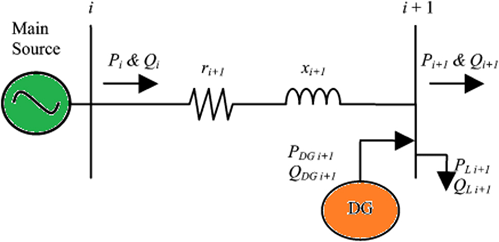
One-line diagram of DG installed in two bus system.
The integration of DG with the distribution system offers quite a few technological and cost-effective profits to utilities and consumers (Mahesh, Nallagownden, and Elamvazuthi 2016). However, the meagre enclosure of DGs may not promise enhancement in system performance. Further, the major advantageous effect of distributed generations depends mainly on its localization and size. Therefore, based on the DGs’ location, size, and diffusion level on the distribution network, the system might negatively influence it. Additionally, to reduce the power loss in power systems, it is merely significant to “define the size and location of distributed generation to be placed”.
In before the improvement of a novel multi-objective based decision-making system for optimal placement of DGs, it is crucial to explore answers to certain critical questions:.
What are the constraints taken into consideration for the optimal placement of DGs?
During the placement of DGs into the balanced/unbalanced distribution feeders, the power loss automatically increases, and how can it be suppressed?
How the system voltage profile enhanced and what is done to retain the voltage of each bus within a permissible range?
Is it possible to diminish the genuine power loss of the system without going against the system limitations, and how is it possible?
As a solution to all these questions, this research work intends to develop a novel multi-objective-based optimization approach.
Proposed solution for optimal placement of DGs
A successful technique is introduced here for “optimal allocation (positioning) and sizing of voltage-controlled DGs using a novel hybrid algorithm”. The main objective of the suggested model is to reduce power loss while increasing the reliability and efficiency of voltage-controlled DGs in unbalanced distribution networks. The suggested multi-objective optimisation method is innovative in that it is created by integrating the LA and SLnO. In proposed multi-objective optimization, the DG is modelled as a “voltage controlled (PV) node with the flexibility to be converted to constant power (PQ) node in case of reactive power limit violation”. Figure 2 shows the schematic diagram of the model that is being given.

Block diagram of the proposed model.
Modelling of distributed generations and load flow study
Modelling of DGs
In a distribution system, the count of DG allocation highly depends on the load demand of the system and the maximum allowable size of DG (Ramamoorthy and Ramachandran 2016). “The maximum allowable size of DG is up to 25–30% of the total load”. Here, the IEEE-123 feeder system is taken into consideration. It is proposed to select a maximum of 5 DGs and a minimum of 2 DGs. The most favorable dimension of DG to be located at each one bus is established out using the proposed multi-objective optimization algorithm. In general, DG is categorized into 2 piece, from the energy source to the point of view. “One is non-renewable energy including cogeneration, fuel cells and microturbine systems and the other is renewable energy including photovoltaic, wind, geothermal, biomass and so on”.
Similar to the central generation, the DG source is also an active power constraint and it is formulated as per Eq. (1).
P gi → Real power production accessible at i th bus.
Because the energy source at any given site intrinsically limits DG capacity, the DG capacity limitation must be calculated between the min and max generation in accordance with Eq. (2).
Moreover, the reactive power output is also important, and it is also taken into consideration as per Eq. (3).
Q gi →Reactive power supplied from i th bus.
Further, to improve the voltage profile as well as voltage at every one bus is obliged to be maintained inside the restrictions as per Eq. (4).
Where,
In the current research work, the voltage limit is set as
Three types of DGs for two DG models are discussed below:
Case 1: These types of DGs generate only real power (e.g. Photovoltaic). A bus i, the best possible size of DG, is found by adjusting its generated real power within the maximal
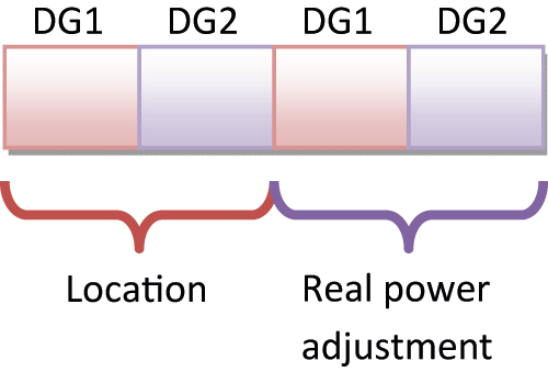
Case 1: Real power adjustment in two DG system (type 1).
Case 2: “The synchronous condenser DG generates only the reactive power” and it is adjusted to get better the voltage profile. A reactive power is adjusted within limits within the maximal
Where, V i,ref → Rated Voltage at bus i.

Case 2: Reactive power adjustment in two DG system (type 2). The voltage profile enhancement V PE is given as per Eq. (5).
Case 3: This type of DG supplies “real power and in turn consume the reactive power”. When it comes to wind turbines, the real power is generated by induction generators and the reactive power will be obsessive here. Therefore, the adjustment is made in both the real and reactive power. Real and reactive power adjustment in two DG system (Type 3) is shown in Figure 5.
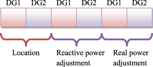
Case 3: Real and reactive power adjustment in two DG system (type 3).
Then, to again establish the most advantageous placement of DG with a minimum loss, the load flow analysis is computed. The connection between the bus system and DGs is modelled using the load flow analysis that is based on the backward, forward sweep method.
Load flow study
The active and reactive power in an ac power system typically flows from the generating station to the load via diverse bus networks and branches (Rajeshkumar and Sujatha 2019). “The flow of active and reactive power is called power flow or load flow”. The load-flow study’s main goal is to provide information on:
Phase angle & voltage magnitude at every bus.
A flow of “Real and Reactive power” in every element.
Calculating the “real and reactive power” flow passing through each line is significantly simpler once the voltage phase angle have been determined. Further, concerning a power flow difference between the sending and the receiving ends, the line losses can be calculated at each of the lines. This helps determine the most favourable position and the most advantageous ability of the presented generating station substation and new lines. The following “power-flow formulae” are used when putting the DGs into the system at various locations expressed in Eq. (6) and Eq. (7) should be satisfied.
Where,
The “backward forward sweep method” is picked for power flow development in the current research work. This approach involves no matrix inversions with limited matrix operations. The two major steps of backward, forward sweep method are:.
Step 1: “backward sweep step→ the branch current” here is computed using KCL depending on node currents.
Step 2: “forward sweep step→ at every nodes”, the updated voltages are computed using KVL.
Realization of DG-based DG placement
The decision-making process in the most favourable assignment of DGs is based on the proposed multi-objective optimization algorithm. The overall steps are shown below:
Step 1: Initially, the DG is placed at a location, and its reactive, real, or real + reactive power is adjusted within the minimal and maximal limits.
Step 2: Then, the power loss P loss is computed using the power flow analysis.
Step 3: The voltage limit and power loss P loss is verified to be minimal, which is the objective function. A penalty function is added if the voltage goes beyond or below the limit.
Step 4: This penalty function and P loss is fed as input to suggested plan for minimization. This helps in the optimal placement of DGs.
Objective function and proposed multi-objective optimization approach
Objective function and solution encoding
The multi-objective optimisation method MUHM that has been devised serves as the foundation for the decision-making process for the best placement of DGs. Here, the power loss as well as the penalty function are quite important. Minimizing “the quantity of real power loss inside the distribution system in addition to the penalty function” is the main goal of the current study activity. The objective function Obj is expressed mathematically as per Eq. (8)
“The losses associated with each branch are computed and summed to calculate the system’s total real power loss”. The equation for total real power loss P loss is depicted in Eq. (9).
Where, N b indicates the number of bus. To achieve this objective, the penalty and P loss are fed as the solution to the proposed MUHM algorithm as illustrated in Figure 6.
Proposed MUHM optimization algorithm
The aforementioned optimisation problem is addressed in this work by the development of the innovative algorithm known as MUHM, an enhanced version of the LA model, and the SLnO model. The most intelligent animals, sea lions, provided the raw inspiration that led to the development of the classic SLnO. While LA is based on the “lion’s unique characteristics such as territorial defense and territorial take over” (George and Rajakumar 2013; Rajakumar 2013; Swamy, Rajakumar, and Valarmathi 2013).
The mathematical process of the developed optimization concept is depicted below:
Step 1: Total population Pop of result P
loss as well as penalty was initialized as t = 1:Pop. Also along with terrestrial lion (both male X
Ma and female X
Fe), a nomadic lions were initialized. Additionally, the SLnO model represents the separation in between target prey as well as the sea as
Step 2: For the current iteration t, if
Equation for
The resultant of the female update
Step 3: If
The very next step represented as (t + 1) and here, the value of
Step 4: If
Dwindling encircling approach:
Circle updating position: This mechanism of the sea lions is modeled mathematically as per Eq. (15). Here, the detachment in flanked by the excited solution (target prey) and the search agent (sea lion) is symbolized as
(15)

Solution encoding.
The resultant acquired in the exploration phase is stored in
Step 5: The leftover solutions are updated by SLnO exploitation phase. This process is expressed mathematically in Eq. (16) and Eq. (17), respectively.
A pseudo-code of proposed model is shown in Algorithm 1.

The flow chart of the proposed model is shown in Figure 7.

Flow chart of proposed MUHM model.
Results and discussion
Simulation procedure
MATLAB was used to develop the suggested hybrid optimisation techniques for the best location and sizing of voltage-controlled generating units in unbalanced distribution networks. On an IEEE bus test system, the created method MUHM is put to the test. Additionally, a contrast of the suggested method with well-known optimisation methods as SFF, BBO, BAT, LA, and SLnO shows that it effectively reduces power losses. Application of the suggested method to various IEEE test systems, including IEEE 33, IEEE 123, and IEEE 69, respectively, is used to assess its efficacy. The evaluation is completed for DG = 1, DG = 2, and DG = 3 in case of Power loss. The highest count of DG is fixed at 3. Since, three different types of DG are modelled here, the evaluation is done under each case. The evaluation is carried out for each scenario because there are three different forms of DG modelled here. The simulation’s inputs are displayed in Table 2.
Simulation parameter.
| Algorithm | Parameters |
|---|---|
| FireFly | Alpha = 0.5; betamin = 0.2; gamma = 1 |
| BBO | KeepRate = 0.2 |
| Alpha = 0.9 | |
| pMutation = 0.1 | |
| BAT | A = 0.5 r = 0.5 |
| Q min = 0 | |
| Q max = 2 | |
| LA | Mature_age = 3 maxium strength = 3 |
| Gmax = 10 | |
| mutation_rate = 0.15 | |
| Maxium age = 3 | |
| Male rate = 0.15 | |
| Female rate = 0.15 | |
| SLnO |
|
|
|
|
| Proposed |
|
|
|
Power loss evaluation for case 1, case2 and case 3: DG count Versus power loss
The real power is changed and the power loss is assessed for several IEEE test systems, including IEEE 33, IEEE 123, and IEEE 69, in the event of DG type 1. The acquired results are represented visually in Figure 8. The submitted approach, with DG = 1, achieves the lowest power loss in Figure 8(a), which corresponds to the IEEE 33 bus system. Overall, the power loss for the suggested model, MUHM, is reduced when compared to the current model, demonstrating its effectiveness. On observing Figure 8(b), the lowest power is achieved by the presented work and at DG = 2, the presented work MUHM is 2, 3, 2.3, 4 and 4.2% better than SFF, BBO, BAT, LA and SLnO, respectively. In Figure 8(c), the presented work achieved the lowest power loss in the case of the varying count of DGs. The lowest power loss is achieved by the presented work at DG = 2.
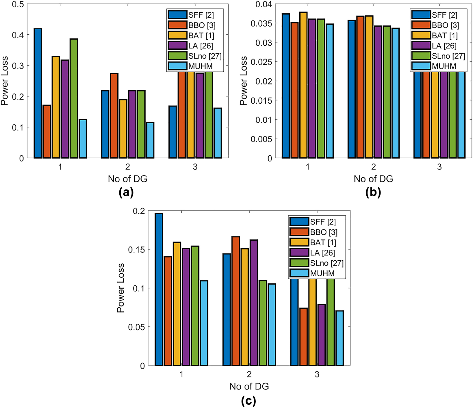
Power loss versus DG count evaluation for type 1 DG (case 1) for (a) IEEE 33, (b) IEEE 123 and (c) IEEE 69.
Figure 9 exhibits the evaluation of suggested plan over the existing work for type 2 DGs (case 2). On observing Figure 9(b), the presented work has achieved the lowest power loss, and at DG = 1, the presented work is 5, 4.8, 9, 6 and 5% better than existing SFF, BBO, BAT, LA and SLnO, respectively. Then, on observing Figure 9(b) and Figure 9(c) corresponding to IEEE 123 and IEEE 69, the presented work achieves the lowest power loss.

Power loss versus DG count evaluation for type 2 DG (case 2) for (a) IEEE 33, (b) IEEE 123 and (c) IEEE 69.
Then, the suggested scheme contrasting with existing work for type 3 DGs (case 3). Here, the lowest power loss is recorded in Figure 10(a) when DG = 1. In situation of IEEE 123 bus system, the presented work achieves the lowest power loss when DG = 2 and it is 2, 1.3, 2.3, 4 and 6% better than SFF, BBO, BAT, LA and SLnO, respectively. In Figure 10(c), the lowest power loss is recorded by the presented work when DG = 3. It is clear from the overall assessment that the work presented has produced the least amount of power loss.

Power loss versus DG count evaluation for type 3 DG (case 3) for (a) IEEE 33, (b) IEEE 123 and (c) IEEE 69.
Power loss evaluation for case 1, case 2 and case 3: loading versus power loss
Figure 11 shows the loading versus power loss for suggested scheme over the traditional job for different IEEE test systems like IEEE 33, IEEE 123 and IEEE 69, respectively, for type 1 DG (case 1). The loading percentage (LP) is varied from 0 to 40. In Figure 11(a) and Figure 11(b), the lowest power is achieved in IEEE 33 and IEEE 123 bus networks in all variations in the loading percentage. Then, in the case of Figure 12(a), the lowest power loss is recorded at LP = 0 and it is 5, 8.6, 4, 5.6 and 9% better than traditional SFF, BBO, BAT, LA and SLnO, respectively. Then, in the case of Figure 12(b) corresponding to type 2 DG (Case 2), the presented work achieves the lowest power loss in case of all the variations in the loading percentage. Similar to this, the presented work achieves the lowest power loss in IEEE 69 bus network in the case of each variation in the loading percentage. Figure 13 shows the power loss evaluation for variation in the loading percentage for case 3 DGs. In Figure 13(a), the lowest power is achieved by the presented work at loading percentage = 0 and it is 12%, 15%, 135, 4.65%, and 8% better than SFF, BBO, BAT, LA and SLnO, respectively. Similar to this, the suggested plan achieves the lowest power loss for every variance in the loading percentage in IEEE 123 and IEEE 69, respectively.
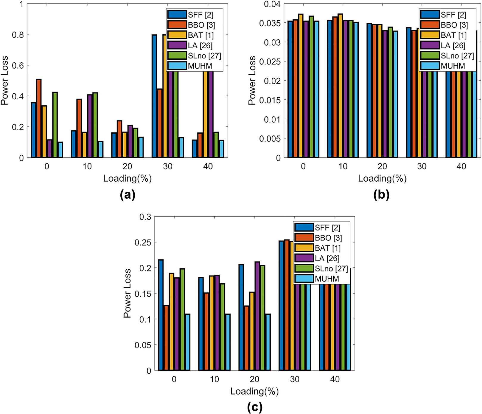
Power loss versus loading factor evaluation for type 1 DG (case 1) for (a) IEEE 33, (b) IEEE 123 and (c) IEEE 69.
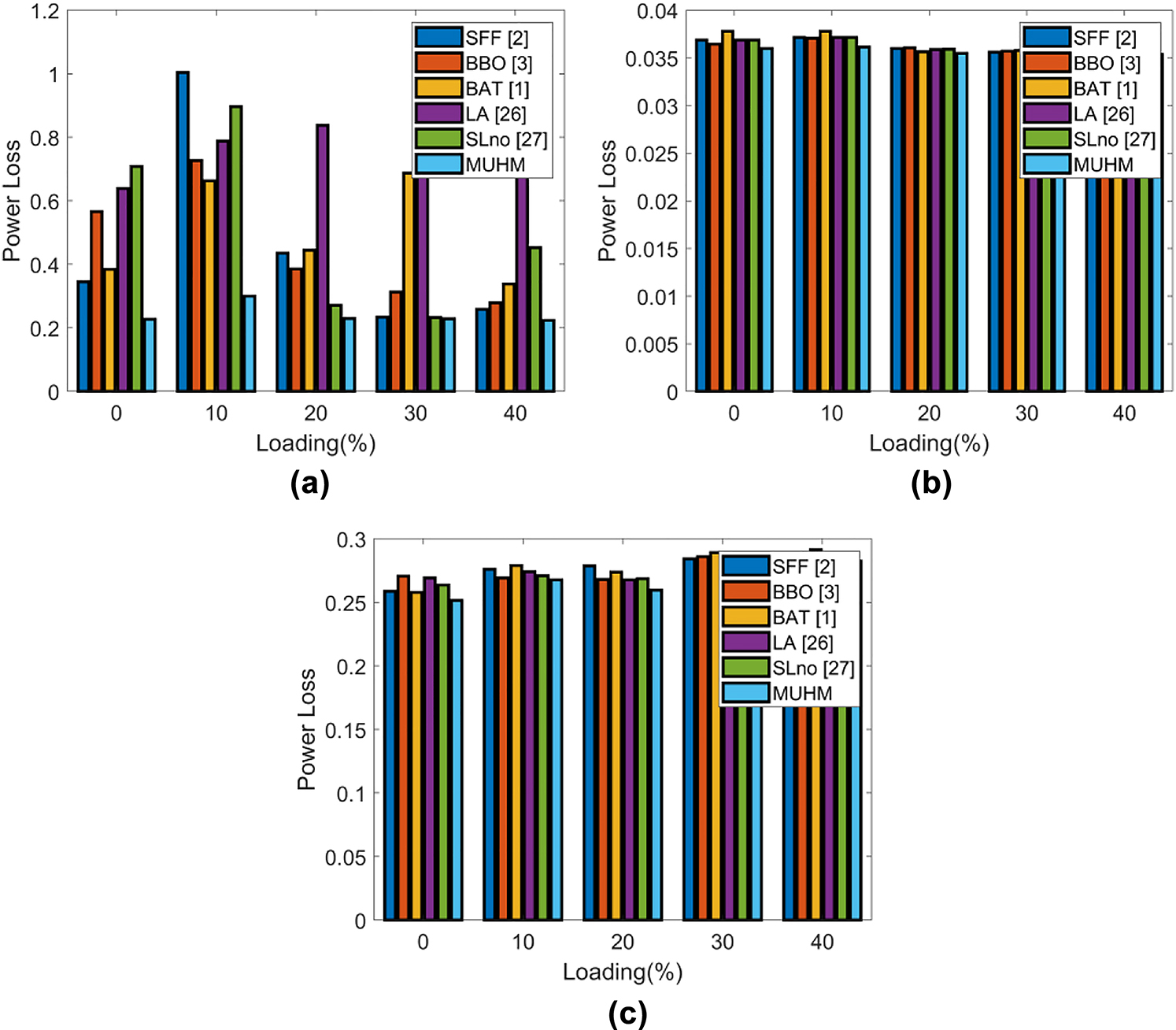
Power loss versus loading factor evaluation for type 2 DG (case 2) for (a) IEEE 33, (b) IEEE 123 and (c) IEEE 69.
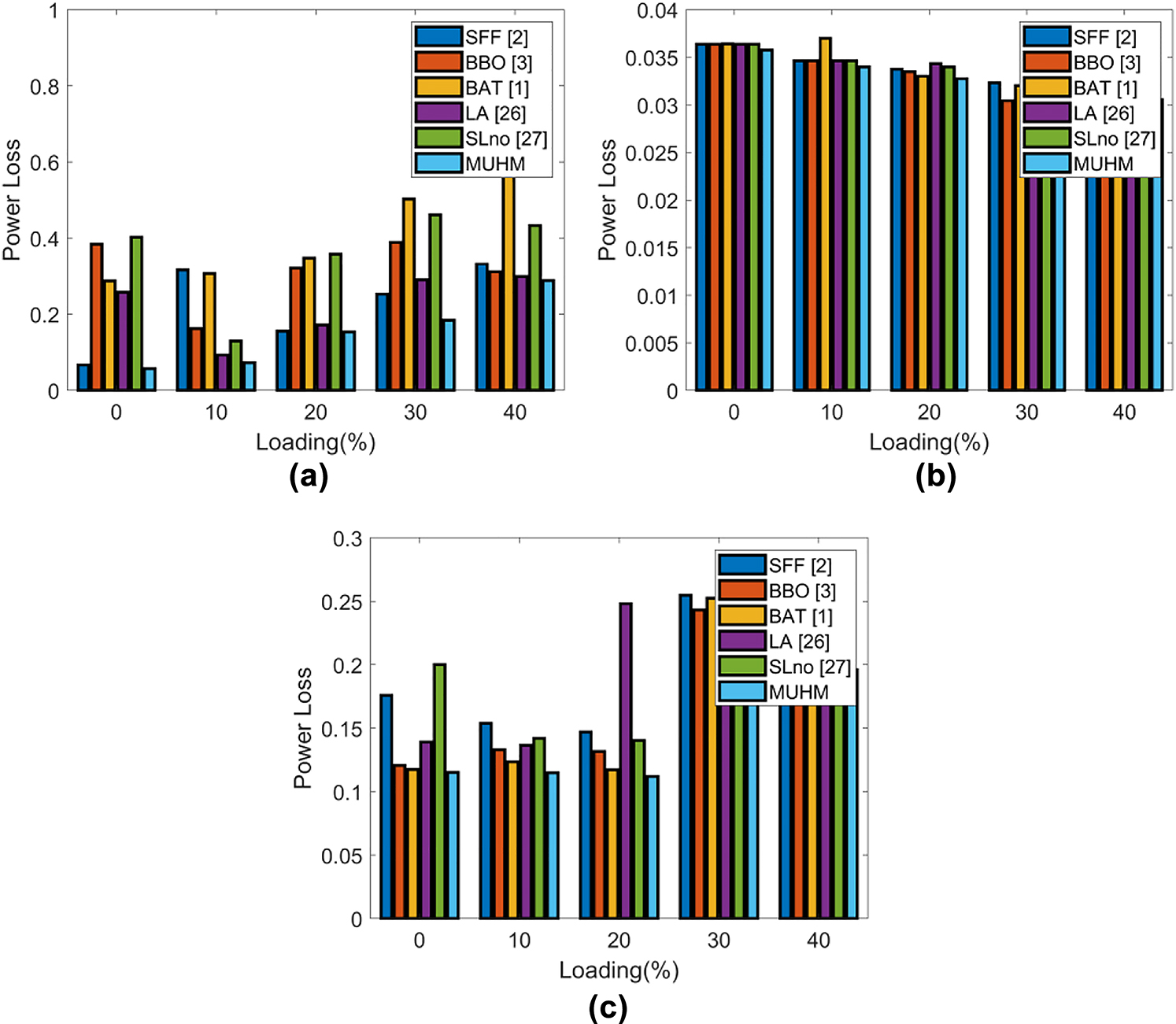
Power loss versus loading factor evaluation for type 3 DG (case 3) for (a) IEEE 33, (b) IEEE 123 and (c) IEEE 69.
Real power evaluation for case1, case 2, and case 3
A presented work acquired the optimal values over existing works for optimal localization of DG at various locations. Table 3 shows the optimal resultant for type 1 DGs corresponding to IEEE bus 69. The resultant real power (P) acquired at each location is shown. When, DG = 2, the real power 0.12 is acquired by the presented work at the location (loc) = 64. Then, When DG = 3, the real power is acquired as 0.078719, 0.067731, and 0.11689 at locations 64, and 62.
Real Power (P) and Reactive power (Q) for optimal localization of DG under Type 1 and Type II for IEEE-69 bus system.
| Type 1 | ||||||||||||||||||
|---|---|---|---|---|---|---|---|---|---|---|---|---|---|---|---|---|---|---|
| Methods | DG = 2 | DG = 3 | DG = 4 | |||||||||||||||
| Loc | P | Loc | P | Loc | P | Loc | P | Loc | P | Loc | P | Loc | P | Loc | P | Loc | P | |
| SFF (Othman et al. 2016) | 27 | 0.047 | 65 | 0.091 | 63 | 0.061 | 65 | 0.09 | 12 | 0.0724 | 16 | 0.076 | 64 | 0.103 | 14 | 0.013 | 21 | 0.107 |
| BBO (Ravindran and Victoire 2018) | 64 | 0.12 | 65 | 0.0641 | 64 | 0.113 | 65 | 0.0949 | 63 | 0.117 | 24 | 0.120 | 21 | 0.112 | 64 | 0.112 | 18 | 0.11 |
| BAT (Sudabattula and Kowsalya 2016) | 64 | 0.12 | 65 | 0.064 | 64 | 0.113 | 65 | 0.095 | 63 | 0.117 | 24 | 0.12 | 21 | 0.112 | 64 | 0.12 | 18 | 0.11 |
| LA (Boothalingam 2018) | 64 | 0.12 | 20 | 0.073 | 1 | 0.017 | 13 | 0.12 | 65 | 0.12 | 64 | 0.12 | 29 | 0.12 | 69 | 0.002 | 69 | 0.12 |
| SLnO (Masadeh, Mahafzah, and Sharieh 2019) | 69 | 0.12 | 65 | 0.12 | 65 | 0.11557 | 27 | 0.10391 | 69 | 0.12 | 65 | 0.086868 | 56 | 0.12 | 69 | 0.12 | 69 | 0.12 |
| MUHM | 65 | 0.103 | 56 | 0.114 | 13 | 0.045 | 19 | 0.033 | 65 | 0.12 | 64 | 0.089 | 57 | 0.12 | 69 | 0.057 | 65 | 0.12 |
| Type 2 | ||||||||||||||||||
|---|---|---|---|---|---|---|---|---|---|---|---|---|---|---|---|---|---|---|
| Methods | DG = 2 | DG = 3 | DG = 4 | |||||||||||||||
| Loc | Q | Loc | Q | Loc | Q | Loc | Q | Loc | Q | Loc | Q | Loc | Q | Loc | Q | Loc | Q | |
| SFF (Othman et al. 2016) | 56 | 0.083 | 20 | 0.071 | 55 | 0.111 | 56 | 0.030 | 54 | 0.045 | 46 | 0.061 | 56 | 0.100 | 25 | 0.090 | 27 | 0.085 |
| BBO (Ravindran and Victoire 2018) | 27 | 0.120 | 64 | 0.110 | 26 | 0.114 | 27 | 0.108 | 17 | 0.114 | 27 | 0.109 | 56 | 0.071 | 26 | 0.113 | 21 | 0.101 |
| BAT (Sudabattula and Kowsalya 2016) | 64 | 0.120 | 69 | 0.120 | 13 | 0.120 | 36 | 0.018 | 27 | 0.120 | 69 | 0.118 | 56 | 0.088 | 24 | 0.12 | 68 | 0.051 |
| LA (Boothalingam 2018) | 69 | 0.069 | 64 | 0.120 | 26 | 0.112 | 65 | 0.082 | 39 | 0.120 | 21 | 0.12 | 27 | 0.12 | 26 | 0.12 | 56 | 0.118 |
| SLnO (Masadeh, Mahafzah, and Sharieh 2019) | 27 | 0.111 | 32 | 0.032 | 63 | 0.119 | 68 | 0.115 | 16 | 0.091 | 69 | 0.12 | 64 | 0.090 | 27 | 0.12 | 69 | 0.059 |
| MUHM | 56 | 0.120 | 27 | 0.120 | 27 | 0.12 | 56 | 0.120 | 26 | 0.120 | 123 | 0.12 | 38 | 0.12 | 16 | 0.12 | 68 | 0.12 |
In Table 4, the real power (P) and reactive power (Q) for the IEEE-69 bus system’s Type III for DG = 2 are displayed. When DG = 2, location 65’s actual and reactive power, respectively, are 0.12 and 0.10961. The actual and reactive power of the activity that is being provided at site 24 is then 0.06284 and 0.082147, accordingly, when DG = 3. Then, at optimal location 61, the real power is 0.091612 and the reactive power is 0.084255. Table 5 displays the real power (P) and reactive power (Q) for the best localisation of the DG under Type III for the IEEE-69 bus system for DG = 3.
Real Power (P) and Reactive power (Q) for optimal localization of DG under Type III for IEEE-69 bus system for DG = 2.
| Methods | DG = 2 | |||||
|---|---|---|---|---|---|---|
| Location | P | Q | Location | P | Q | |
| SFF (Othman et al. 2016) | 65 | 0.072481 | 0.084928 | 25 | 0.070414 | 0.047011 |
| BBO (Ravindran and Victoire 2018) | 65 | 0.11591 | 0.088017 | 7 | 0.072972 | 0.021979 |
| BAT (Sudabattula and Kowsalya 2016) | 69 | 0.052181 | 0.12 | 61 | 0.12 | 0.12 |
| LA (Boothalingam 2018) | 64 | 0.12 | 0.12 | 65 | 0.12 | 0.12 |
| SLnO (Masadeh, Mahafzah, and Sharieh 2019) | 69 | 0.029481 | 0.12 | 26 | 0.084681 | 0.1015 |
| MUHM | 65 | 0.12 | 0.10961 | 24 | 0.0843 | 0.09549 |
Real Power (P) and Reactive power (Q) for optimal localization of DG under Type III for IEEE-69 bus system for DG = 3.
| Methods | DG = 3 | ||||||||
|---|---|---|---|---|---|---|---|---|---|
| Location | P | Q | Location | P | Q | Location | P | Q | |
| SFF (Othman et al. 2016) | 22 | 0.056568 | 0.077265 | 21 | 0.049068 | 0.032575 | 26 | 0.071566 | 0.032664 |
| BBO (Ravindran and Victoire 2018) | 21 | 0.079832 | 0.081072 | 20 | 0.11987 | 0.076709 | 64 | 0.076723 | 0.02357 |
| BAT (Sudabattula and Kowsalya 2016) | 1 | 0.11994 | 0.12 | 7 | 0.12 | 0.05785 | 65 | 0.12 | 0.061165 |
| LA (Boothalingam 2018) | 65 | 0.11531 | 0.11492 | 11 | 0.11395 | 0.09025 | 63 | 0.11348 | 0.059721 |
| SLnO (Masadeh, Mahafzah, and Sharieh 2019) | 26 | 0.074117 | 0.10754 | 22 | 0.057936 | 0.060953 | 65 | 0.093483 | 0.078027 |
| MUHM | 24 | 0.06284 | 0.082147 | 61 | 0.091612 | 0.084255 | 65 | 0.066121 | 0.10513 |
The real power and reactive power for optimal localization of DG under Type III for IEEE-69 bus system for DG = 4 is shown in Table 6. When DG = 4, the real and the reactive power of the presented work is 0.092624 and 0.06572 at optimal location 33.
Real Power (P) and Reactive power (Q) for optimal localization of DG under Type III for IEEE-69 bus system for DG = 4.
| Methods | DG = 4 | |||||||||||
|---|---|---|---|---|---|---|---|---|---|---|---|---|
| Location | P | Q | Location | P | Q | Location | P | Q | Location | P | Q | |
| SFF (Othman et al. 2016) | 43 | 0.032 | 0.023 | 13 | 0.087 | 0.102 | 64 | 0.054 | 0.076 | 65 | 0.099 | 0.082 |
| BBO (Ravindran and Victoire 2018) | 27 | 0.052 | 0.045 | 56 | 0.100 | 0.107 | 65 | 0.038 | 0.079 | 64 | 0.047 | 0.054 |
| BAT (Sudabattula and Kowsalya 2016) | 1 | 0.086 | 0.006 | 1 | 0.120 | 0.120 | 69 | 0.017 | 0.093 | 61 | 0.120 | 0.047 |
| LA (Boothalingam 2018) | 22 | 0.010 | 0.024 | 4 | 0.091 | 0.106 | 65 | 0.043 | 0.071 | 64 | 0.111 | 0.086 |
| SLnO (Masadeh, Mahafzah, and Sharieh 2019) | 22 | 0.017 | 0.027 | 18 | 0.095 | 0.107 | 65 | 0.053 | 0.072 | 63 | 0.116 | 0.091 |
| MUHM | 33 | 0.093 | 0.066 | 26 | 0.075 | 0.096 | 62 | 0.119 | 0.092 | 64 | 0.006 | 0.057 |
In Tables 7 and 8, the Real Power (P) & Reactive Power (Q) for DG = 2, DG = 3, and DG = 4 optimal localisation within Type I and Type II for IEEE-33 bus system are shown. On noticing Table 8, at location 24, for DG = 1 belonging to type I, the proposed model consumes the reactive power of 0.069497 at location 24. Table 9 shows the actual power (P) & reactive power (Q) for the best localisation of the DG under Type III for the IEEE-33 bus system for DG = 2, and DG = 3.
Real Power (P) for optimal localization of DG under Type I for IEEE-33 bus system for DG = 2, DG = 3 and DG = 4.
| Methods | DG = 2 | DG = 3 | DG = 4 | |||||||||||||||
|---|---|---|---|---|---|---|---|---|---|---|---|---|---|---|---|---|---|---|
| Loc | P | Loc | P | Loc | P | Loc | P | Loc | P | Loc | P | Loc | P | Loc | P | Loc | P | |
| SFF (Othman et al. 2016) | 33 | 0.102 | 33 | 0.12 | 12 | 0.100 | 20 | 0.083 | 7 | 0.077 | 27 | 0.023 | 14 | 0.097 | 18 | 0.0703 | 12 | 0.12 |
| BBO (Ravindran and Victoire 2018) | 20 | 0.048 | 12 | 0.105 | 12 | 0.050 | 16 | 0.045 | 13 | 0.010 | 7 | 0.017 | 9 | 0 | 4 | 0.0312 | 10 | 0.093 |
| BAT (Sudabattula and Kowsalya 2016) | 20 | 0.120 | 33 | 0.085 | 12 | 0.111 | 20 | 0.049 | 9 | 0.094 | 1 | 0.000 | 20 | 0.108 | 33 | 0.0959 | 33 | 0.100 |
| LA (Boothalingam 2018) | 33 | 0.082 | 20 | 0.119 | 12 | 0.100 | 20 | 0.083 | 7 | 0.077 | 51 | 0.088 | 20 | 0.107 | 11 | 0.0907 | 33 | 0.074 |
| SLnO (Masadeh, Mahafzah, and Sharieh 2019) | 20 | 0.068 | 33 | 0.113 | 12 | 0.100 | 20 | 0.083 | 7 | 0.077 | 44 | 0.072 | 20 | 0.080 | 26 | 0.0609 | 33 | 0.12 |
| MUHM | 12 | 0.097 | 18 | 0.076 | 7 | 0.082 | 17 | 0.065 | 12 | 0.088 | 51 | 0.059 | 25 | 0.039 | 9 | 0.0656 | 12 | 0.082 |
Reactive Power (Q) for optimal localization of DG under Type II for IEEE-33 bus system for DG = 2, DG = 3 and DG = 4.
| Methods | DG = 2 | DG = 3 | DG = 4 | |||||||||||||||
|---|---|---|---|---|---|---|---|---|---|---|---|---|---|---|---|---|---|---|
| Loc | Q | Loc | Q | Loc | Q | Loc | Q | Loc | Q | Loc | Q | Loc | Q | Loc | Q | Loc | Q | |
| SFF (Othman et al. 2016) | 13 | 0.021 | 5 | 0.015 | 2 | 0.112 | 11 | 0.042 | 13 | 0.015 | 39 | 0.066 | 20 | 0.112 | 12 | 0.080 | 14 | 0.1178 |
| BBO (Ravindran and Victoire 2018) | 33 | 0.049 | 12 | 0.073 | 13 | 0.017 | 30 | 0.065 | 16 | 0.069 | 39 | 0.091 | 25 | 0.028 | 12 | 0.085 | 8 | 0.0147 |
| BAT (Sudabattula and Kowsalya 2016) | 33 | 0.058 | 12 | 0.085 | 5 | 0.117 | 2 | 0.117 | 13 | 0.016 | 56 | 0.088 | 20 | 0.002 | 12 | 0.118 | 33 | 0.0248 |
| LA (Boothalingam 2018) | 33 | 0.091 | 12 | 0.075 | 4 | 0.109 | 21 | 0.044 | 13 | 0.015 | 39 | 0.113 | 16 | 0.005 | 20 | 0.110 | 32 | 0.0086 |
| SLnO (Masadeh, Mahafzah, and Sharieh 2019) | 1 | 0 | 13 | 0.018 | 4 | 0.110 | 2 | 0.011 | 13 | 0.015 | 54 | 0.119 | 26 | 0.015 | 27 | 0.119 | 33 | 0.0938 |
| MUHM | 24 | 0.069 | 12 | 0.0624 | 12 | 0.094 | 25 | 0.103 | 22 | 0.033 | 39 | 0.113 | 18 | 0.007 | 12 | 0.116 | 32 | 0.0378 |
Real Power (P) and Reactive power (Q) for optimal localization of DG under Type III for IEEE-33 bus system for DG = 2, and DG = 3.
| Methods | DG = 2 | DG = 3 | |||||||||||||
|---|---|---|---|---|---|---|---|---|---|---|---|---|---|---|---|
| Loc | P | Q | Loc | P | Q | Loc | P | Q | Loc | P | Q | Loc | P | Q | |
| SFF (Othman et al. 2016) | 12 | 0.069 | 0.064 | 29 | 0.065 | 0.082 | 19 | 0.100 | 0.045 | 12 | 0.094 | 0.038 | 24 | 0.085 | 0.077 |
| BBO (Ravindran and Victoire 2018) | 12 | 0.069 | 0.064 | 29 | 0.065 | 0.082 | 23 | 0.114 | 0.037 | 26 | 0.101 | 0.068 | 12 | 0.117 | 0.077 |
| BAT (Sudabattula and Kowsalya 2016) | 12 | 0.029 | 0.033 | 29 | 0.110 | 0.088 | 16 | 0.120 | 0.120 | 20 | 0.120 | 0.120 | 10 | 0.120 | 0.120 |
| LA (Boothalingam 2018) | 12 | 0.069 | 0.064 | 29 | 0.065 | 0.082 | 1 | 0.114 | 0.095 | 9 | 0.066 | 0.047 | 33 | 0.116 | 0.071 |
| SLnO (Masadeh, Mahafzah, and Sharieh 2019) | 12 | 0.088 | 0.071 | 32 | 0.067 | 0.100 | 20 | 0.120 | 0.087 | 25 | 0.114 | 0.087 | 14 | 0.120 | 0.120 |
| MUHM | 12 | 0.052 | 0.066 | 25 | 0.054 | 0.038 | 18 | 0.095 | 0.102 | 12 | 0.097 | 0.014 | 17 | 0.045 | 0.080 |
The real power (P) and reactive power (Q) for optimal localization of DG under Type III for IEEE-33 bus system for DG = 4 is illustrated in Table 10.
Real Power (P) and Reactive power (Q) for optimal localization of DG under Type III for IEEE-33 bus system for DG = 4.
| Methods | DG = 4 | |||||||||||
|---|---|---|---|---|---|---|---|---|---|---|---|---|
| Loc | P | Q | Loc | P | Q | Loc | P | Q | Loc | P | Q | |
| SFF (Othman et al. 2016) | 25 | 0.073 | 0.084 | 12 | 0.026 | 0.074 | 19 | 0.100 | 0.041 | 12 | 0.013 | 0.100 |
| BBO (Ravindran and Victoire 2018) | 25 | 0.073 | 0.084 | 12 | 0.026 | 0.074 | 19 | 0.100 | 0.041 | 12 | 0.013 | 0.100 |
| BAT (Sudabattula and Kowsalya 2016) | 25 | 0.070 | 0.083 | 11 | 0.025 | 0.074 | 18 | 0.095 | 0.037 | 12 | 0.008 | 0.100 |
| LA (Boothalingam 2018) | 25 | 0.073 | 0.084 | 12 | 0.026 | 0.074 | 19 | 0.100 | 0.041 | 12 | 0.013 | 0.100 |
| SLnO (Masadeh, Mahafzah, and Sharieh 2019) | 25 | 0.072 | 0.084 | 11 | 0.026 | 0.074 | 19 | 0.099 | 0.040 | 12 | 0.011 | 0.100 |
| MUHM | 28 | 0.102 | 0.117 | 4 | 0.005 | 0.12 | 13 | 0.082 | 0.055 | 14 | 0.007 | 0.111 |
The real power (P) for optimal localization of DG under Type I for IEEE-123 bus system for DG = 2, DG = 3 and DG = 4 is depicted in Table 11. The reactive power (Q) for optimal localization of DG under Type I for the IEEE-123 bus system for DG = 2, DG = 3, and DG = 4 is shown in Table 12.
Real Power (P) for optimal localization of DG under Type I for IEEE-123 bus system for DG = 2, DG = 3 and DG = 4.
| Methods | DG = 2 | DG = 3 | DG = 4 | |||||||||||||||
|---|---|---|---|---|---|---|---|---|---|---|---|---|---|---|---|---|---|---|
| Loc | P | Loc | P | Loc | P | Loc | P | Loc | P | Loc | P | Loc | P | Loc | P | Loc | P | |
| SFF (Othman et al. 2016) | 43 | 0.025 | 4 | 0.036 | 33 | 0.0007 | 5 | 0.016 | 38 | 0.107 | 26 | 0.0002 | 21 | 0.062 | 2 | 0.088 | 22 | 0.078 |
| BBO (Ravindran and Victoire 2018) | 27 | 0.070 | 11 | 0.087 | 44 | 0.0204 | 53 | 0.029 | 2 | 0.053 | 49 | 0.114 | 40 | 0.096 | 12 | 0.006 | 45 | 0.088 |
| BAT (Sudabattula and Kowsalya 2016) | 1 | 0.118 | 1 | 0 | 56 | 0.12 | 56 | 0.119 | 1 | 0.120 | 56 | 0.12 | 56 | 0.12 | 56 | 0 | 56 | 0 |
| LA (Boothalingam 2018) | 22 | 0.071 | 8 | 0.024 | 53 | 0.0543 | 14 | 0.034 | 28 | 0.093 | 18 | 0.108 | 38 | 0.092 | 55 | 0.018 | 34 | 0.046 |
| SLnO (Masadeh, Mahafzah, and Sharieh 2019) | 22 | 0.071 | 8 | 0.024 | 53 | 0.0543 | 14 | 0.034 | 28 | 0.093 | 12 | 0.101 | 34 | 0.037 | 8 | 0.046 | 27 | 0.064 |
| MUHM | 33 | 0.069 | 14 | 0.109 | 35 | 0.1024 | 53 | 0.099 | 51 | 0.023 | 18 | 0.108 | 38 | 0.092 | 55 | 0.018 | 34 | 0.046 |
Reactive power (Q) for optimal localization of DG under Type I for IEEE-123 bus system for DG = 2, DG = 3, and DG = 4.
| Methods | DG = 2 | DG = 3 | DG = 4 | |||||||||||||||
|---|---|---|---|---|---|---|---|---|---|---|---|---|---|---|---|---|---|---|
| Loc | Q | Loc | Q | Loc | Q | Loc | Q | Loc | Q | Loc | Q | Loc | Q | Loc | Q | Loc | Q | |
| SFF (Othman et al. 2016) | 28 | 0.089 | 3 | 0.077 | 18 | 0.094 | 11 | 0.029 | 44 | 0.098 | 27 | 0.087 | 30 | 0.023 | 9 | 0.087 | 52 | 0.040 |
| BBO (Ravindran and Victoire 2018) | 41 | 0.025 | 2 | 0.035 | 21 | 0.009 | 30 | 0.095 | 33 | 0.063 | 7 | 0.114 | 4 | 0.041 | 12 | 0.109 | 17 | 0.048 |
| BAT (Sudabattula and Kowsalya 2016) | 1 | 0.001 | 1 | 0.12 | 1 | 0 | 56 | 0.12 | 1 | 0 | 1 | 0.001 | 1 | 0.12 | 56 | 0.119 | 1 | 0.003 |
| LA (Boothalingam 2018) | 27 | 0.053 | 26 | 0.110 | 19 | 0.071 | 44 | 0.112 | 29 | 0.038 | 51 | 0.098 | 38 | 0.081 | 33 | 0.101 | 25 | 0.034 |
| SLnO (Masadeh, Mahafzah, and Sharieh 2019) | 4 | 0.050 | 39 | 0.076 | 12 | 0.034 | 36 | 0.109 | 36 | 0.024 | 44 | 0.043 | 36 | 0.081 | 27 | 0.006 | 33 | 0.014 |
| MUHM | 27 | 0.053 | 26 | 0.110 | 19 | 0.071 | 44 | 0.112 | 29 | 0.038 | 51 | 0.098 | 38 | 0.081 | 33 | 0.101 | 25 | 0.034 |
The real Power (P) and reactive power (Q) for optimal localization of DG under Type I for IEEE-123 bus system for DG = 2, and DG = 3 is illustrated in Table 13. The real Power (P) and reactive power (Q) for optimal localization of DG under Type I for IEEE-123 bus system for DG = 4 is depicted in Table 14.
Real Power (P) and Reactive power (Q) for optimal localization of DG under Type I for IEEE-123 bus system for DG = 2, and DG = 3.
| Methods | DG = 2 | DG = 3 | |||||||||||||
|---|---|---|---|---|---|---|---|---|---|---|---|---|---|---|---|
| Loc | P | Q | Loc | P | Q | Loc | P | Q | Loc | P | Q | Loc | P | Q | |
| SFF (Othman et al. 2016) | 10 | 0.084 | 0.004 | 27 | 0.048 | 0.098 | 39 | 0.014 | 0.103 | 52 | 0.096 | 0.112 | 16 | 0.030 | 0.015 |
| BBO (Ravindran and Victoire 2018) | 10 | 0.084 | 0.004 | 27 | 0.048 | 0.098 | 39 | 0.014 | 0.103 | 52 | 0.096 | 0.112 | 16 | 0.030 | 0.015 |
| BAT (Sudabattula and Kowsalya 2016) | 56 | 0.120 | 0.120 | 56 | 0.000 | 0.000 | 56 | 0.000 | 0.000 | 1 | 0.000 | 0.120 | 5 | 0.000 | 0.000 |
| LA (Boothalingam 2018) | 10 | 0.084 | 0.004 | 27 | 0.048 | 0.098 | 39 | 0.014 | 0.103 | 52 | 0.096 | 0.112 | 16 | 0.030 | 0.015 |
| SLnO (Masadeh, Mahafzah, and Sharieh 2019) | 10 | 0.084 | 0.004 | 27 | 0.048 | 0.098 | 54 | 0.001 | 0.058 | 54 | 0.104 | 0.067 | 35 | 0.049 | 0.004 |
| MUHM | 56 | 0.092 | 0.091 | 29 | 0.025 | 0.022 | 39 | 0.014 | 0.103 | 52 | 0.096 | 0.112 | 16 | 0.030 | 0.015 |
Real Power (P) and Reactive power (Q) for optimal localization of DG under Type I for IEEE-123 bus system for DG = 4.
| Methods | DG = 4 | |||||||||||
|---|---|---|---|---|---|---|---|---|---|---|---|---|
| Loc | P | Q | Loc | P | Q | Loc | P | Q | Loc | P | Q | |
| SFF (Othman et al. 2016) | 47 | 0.047984 | 0.041297 | 49 | 0.094528 | 0.11368 | 10 | 0.088361 | 0.043325 | 9 | 0.094947 | 0.042932 |
| BBO (Ravindran and Victoire 2018) | 47 | 0.047984 | 0.041297 | 49 | 0.094528 | 0.11368 | 10 | 0.088361 | 0.043325 | 9 | 0.094947 | 0.042932 |
| BAT (Sudabattula and Kowsalya 2016) | 56 | 0 | 0 | 56 | 0.12 | 0.12 | 1 | 0.12 | 0.12 | 56 | 0 | 0 |
| LA (Boothalingam 2018) | 47 | 0.047984 | 0.041297 | 49 | 0.094528 | 0.11368 | 10 | 0.088361 | 0.043325 | 9 | 0.094947 | 0.042932 |
| SLnO (Masadeh, Mahafzah, and Sharieh 2019) | 49 | 0.097222 | 0 | 50 | 0.073605 | 0.028471 | 8 | 0.028341 | 0.06325 | 21 | 0.02761 | 0.070462 |
| MUHM | 47 | 0.047984 | 0.041297 | 49 | 0.094528 | 0.11368 | 10 | 0.088361 | 0.043325 | 9 | 0.094947 | 0.042932 |
Convergence analysis
Figure 14 shows the convergence evaluation of the proposed MUHM paradigm over the traditional models. On observing Figure 14, when the iteration increases, the proposed MUHM method accomplishes minimum value when compared with other traditional approaches. From Figure 14, at the 40th iteration, the proposed method is 8.158, 6.559, 8.830, 6.927 and 6.582%, superior to SFF, BBO, BAT, LA and SLnO. As a result, the suggested MUHM algorithm’s effectiveness is established.
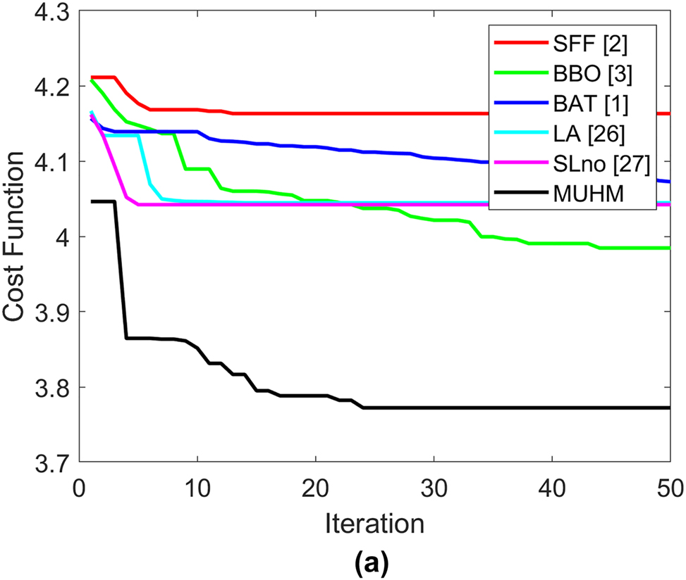
Convergence analysis of the proposed over the conventional models.
Computational time
A computational complexity of presented MUHM algorithm over the other traditional algorithm is illustrated in Table 15. On observing Table 15, Conclusion: When compared to previous algorithms, the suggested hybrid MUHM method computes more quickly. A proposed algorithm is 3.91, 8.51, 2.85, 70.48, and 3.82% better than the conventional SFF, BBO, BAT, LA, and SLnO algorithms.
Computational time of proposed over the conventional models.
| S. No | Methods | Computational time (s) |
|---|---|---|
| 1. | SFF (Othman et al. 2016) | 120.09 |
| 2. | BBO (Ravindran and Victoire 2018) | 126.13 |
| 3. | BAT (Sudabattula and Kowsalya 2016) | 118.79 |
| 4. | LA (Boothalingam 2018) | 390.96 |
| 5. | SLno (Masadeh, Mahafzah, and Sharieh 2019) | 119.99 |
| 6. | MUHM | 115.4 |
Conclusions
In order to minimise power/energy loss while remaining within the bounds of the system, this research effort has developed a novel decision-making technique to identify the ideal sizing and localisation of DGs linked to balanced/unbalanced distribution feeders. The suggested method of generating decisions was based on MUHM, a novel multi-objective optimisation algorithm that combines SLnO with LA. Application to various IEEE test systems, including IEEE 33, IEEE 123, and IEEE 69, served as a gauge of the suggested method’s effectiveness. By using the most modern machine learning algorithm to aid in the fault location, this work’s future directions can be broadened. This suggested MUHM model can be used in the future to size infinite generators with changeable power factor constraints in radial test feeders, such as solar and wind generators. Additionally, a model of this kind will be modified to include capacitors & battery energy storage systems for islanded microgrid uses.
-
Author contributions: All the authors have accepted responsibility for the entire content of this submitted manuscript and approved submission.
-
Research funding: None declared.
-
Conflict of interest statement: The authors declare no conflicts of interest regarding this article.
References
Arkadan, A. A., and M. El Hariri. 2016. “EM–SS-Wavelets for Characterization of High-Speed Generators in Distributed Generation.” IEEE Transactions on Magnetics 52 (3): 1–4. Art no. 8101504, https://doi.org/10.1109/tmag.2015.2477370.Search in Google Scholar
Biswas, P. P., R. Mallipeddi, P. N. Suganthan, and G. A. J. Amaratunga. 2017. “A Multi-Objective Approach for Optimal Placement and Sizing of Distributed Generators and Capacitors in Distribution Network.” Applied Soft Computing 60: 268–80, https://doi.org/10.1016/j.asoc.2017.07.004.Search in Google Scholar
Boothalingam, R. 2018. “Optimization Using Lion Algorithm: A Biological Inspiration from Lion’s Social Behavior.” Evolutionary Intelligence 11 (1–2): 31–52, https://doi.org/10.1007/s12065-018-0168-y.Search in Google Scholar
Chandrashekhar Reddy, S., and P. V. N. Prasad. 2012. “Power Quality Improvement of Distribution System by Optimal Placement of Distributed Generators Using GA and NN.” In Proceedings of the International Conference on Soft Computing for Problem Solving, 257–67. Springer.10.1007/978-81-322-0487-9_25Search in Google Scholar
Gayathri Devi, K. S. 2019. “Hybrid Genetic Algorithm and Particle Swarm Optimization Algorithm for Optimal Power Flow in Power System.” Journal of Computational Mechanics, Power System and Control 2 (2): 31–7, https://doi.org/10.46253/jcmps.v2i2.a4.Search in Google Scholar
George, A., and B. R. Rajakumar. 2013. “APOGA: An Adaptive Population Pool Size Based Genetic Algorithm.” In AASRI Procedia – 2013 AASRI Conference on Intelligent Systems and Control (ISC 2013), Vol. 4, 288–96.10.1016/j.aasri.2013.10.043Search in Google Scholar
Jamil, M., and A. S. Anees. 2016. “Optimal Sizing and Location of SPV (Solar Photovoltaic) Based MLDG (Multiple Location Distributed Generator) in Distribution System for Loss Reduction, Voltage Profile Improvement with Economical Benefits.” Energy 103: 231–9, https://doi.org/10.1016/j.energy.2016.02.095.Search in Google Scholar
Ji, H., C. Wang, P. Li, G. Song, and J. Wu. 2019. “Quantified Analysis Method for Operational Flexibility of Active Distribution Networks with High Penetration of Distributed Generators.” Applied Energy 239: 706–14, https://doi.org/10.1016/j.apenergy.2019.02.008.Search in Google Scholar
Ji, H., C. Wang, P. Li, J. Zhao, and J. Wu. 2018. “A Centralized-Based Method to Determine the Local Voltage Control Strategies of Distributed Generator Operation in Active Distribution Networks.” Applied Energy 228: 2024–36, https://doi.org/10.1016/j.apenergy.2018.07.065.Search in Google Scholar
Mahesh, K., P. Nallagownden, and I. Elamvazuthi. 2016. “Advanced Pareto Front Non-dominated Sorting Multi-Objective Particle Swarm Optimization for Optimal Placement and Sizing of Distributed Generation.” Energies 9 (12): 982, https://doi.org/10.3390/en9120982.Search in Google Scholar
Malhotra, J., and J. Bakal. 2018. “Grey Wolf Optimization Based Clustering of Hybrid Fingerprint for Efficient De-duplication.” Multiagent and Grid Systems 14 (2): 145–60, https://doi.org/10.3233/mgs-180285.Search in Google Scholar
Manickavasagam, K. 2015. “Intelligent Energy Control Center for Distributed Generators Using Multi-Agent System.” IEEE Transactions on Power Systems 30 (5): 2442–9, https://doi.org/10.1109/tpwrs.2014.2368592.Search in Google Scholar
Masadeh, R, A. B. Mahafzah, and A. Sharieh. 2019. “Sea Lion Optimization Algorithm.” International Journal of Advanced Computer Science and Applications (IJACSA) 10 (5): 388–95, https://doi.org/10.14569/ijacsa.2019.0100548.Search in Google Scholar
Mistry, K. D., and R. Roy. 2014. “Enhancement of Loading Capacity of Distribution System through Distributed Generator Placement Considering Techno-Economic Benefits with Load Growth.” International Journal of Electrical Power & Energy Systems 54: 505–15, https://doi.org/10.1016/j.ijepes.2013.07.032.Search in Google Scholar
Mohana, S., and S. S. A. Mary. 2017. “Heuristics for Privacy Preserving Data Mining: An Evaluation.” In 2017 International Conference on Algorithms, Methodology, Models and Applications in Emerging Technologies (ICAMMAET), 1–9: IEEE.10.1109/ICAMMAET.2017.8186664Search in Google Scholar
Mohana, S., S. A. Sahaaya, and A. Mary. 2016. “A Comparitive Framework for Feature Selction in Privacy Preserving Data Mining Techniques Using Pso and K-Anonumization.” Iioab Journal 7 (9): 804–11.Search in Google Scholar
Montoya, O. D., W. Gil-González, and C. Orozco-Henao. 2020. “Vortex Search and Chu-Beasley Genetic Algorithms for Optimal Location and Sizing of Distributed Generators in Distribution Networks: A Novel Hybrid Approach.” Engineering Science and Technology, an International Journal 23 (6): 1351–63, https://doi.org/10.1016/j.jestch.2020.08.002.Search in Google Scholar
Mota, A., L. Mota, and F. Galiana. 2011. “An Analytical Approach to the Economical Assessment of Wind Distributed Generators Penetration in Electric Power Systems with Centralized Thermal Generation.” IEEE Latin America Transactions 9 (5): 726–31, https://doi.org/10.1109/tla.2011.6030982.Search in Google Scholar
Muthukumar, K., and S. Jayalalitha. 2016. “Optimal Placement and Sizing of Distributed Generators and Shunt Capacitors for Power Loss Minimization in Radial Distribution Networks Using Hybrid Heuristic Search Optimization Technique.” International Journal of Electrical Power & Energy Systems 78: 299–319, https://doi.org/10.1016/j.ijepes.2015.11.019.Search in Google Scholar
Nguyen, T. P., T. T. Tran, and D. N. Vo. 2018. “Improved Stochastic Fractal Search Algorithm with Chaos for Optimal Determination of Location, Size, and Quantity of Distributed Generators in Distribution Systems.” Neural Computing and Applications 31 (11): 7707–32, https://doi.org/10.1007/s00521-018-3603-1.Search in Google Scholar
Othman, M. M., W. El-Khattam, Y. G. Hegazy, and A. Y. Abdelaziz. 2016. “Optimal Placement and Sizing of Voltage Controlled Distributed Generators in Unbalanced Distribution Networks Using Supervised Firefly Algorithm.” International Journal of Electrical Power & Energy Systems 82: 105–13, https://doi.org/10.1016/j.ijepes.2016.03.010.Search in Google Scholar
Quattrini, F., A. Ortolani, C. Ciatti, C. P. Pagliarello, A. Martucci, L. Gurrieri, S. Stallone, G. Melucci, T. Domenico, and P. Maniscalco. 2021. “Static vs Dinamic Short Nail in Pertrochanteric Fractures: Experience of Two Center in Northern Italy.” Acta Biomed 92 (S3): e2021021, https://doi.org/10.23750/abm.v92iS3.11745.Search in Google Scholar PubMed PubMed Central
Rajakumar, B. R. 2013. “Impact of Static and Adaptive Mutation Techniques on Genetic Algorithm.” International Journal of Hybrid Intelligent Systems 10 (1): 11–22, https://doi.org/10.3233/his-120161.Search in Google Scholar
Rajeshkumar, G. 2019. “Hybrid Particle Swarm Optimization and Firefly Algorithm for Distributed Generators Placements in Radial Distribution System.” Journal of Computational Mechanics, Power System and Control 2 (1): 41–8, https://doi.org/10.46253/jcmps.v2i1.a5.Search in Google Scholar
Rajeshkumar, G., and T. P. Sujatha. 2019. “Optimal Positioning and Sizing of Distributed Generators Using Hybrid MFO-WC Algorithm.” Journal of Computational Mechanics, Power System and Control 2 (4): 19–27, https://doi.org/10.46253/jcmps.v2i4.a3.Search in Google Scholar
Ramamoorthy, A., and R. Ramachandran. 2016. “Optimal Siting and Sizing of Multiple DG Units for the Enhancement of Voltage Profile and Loss Minimization in Transmission Systems Using Nature Inspired Algorithms.” The Scientific World Journal 2016: 1–16, https://doi.org/10.1155/2016/1086579.Search in Google Scholar PubMed PubMed Central
Rastgou, A., J. Moshtagh, and S. Bahramara. 2018. “Improved Harmony Search Algorithm for Electrical Distribution Network Expansion Planning in the Presence of Distributed Generators.” Energy 151: 178–202, https://doi.org/10.1016/j.energy.2018.03.030.Search in Google Scholar
Ravikumar, S., H. Vennila, and R. Deepak. 2019. “Optimal Positioning of Distributed Generator Using Hybrid Optimization Algorithm in Radial Distribution System.” Journal of Computational Mechanics, Power System and Control 2 (4): 1–9, https://doi.org/10.46253/jcmps.v2i4.a1.Search in Google Scholar
Ravindran, S., and T. A. A. Victoire. 2018. “A Bio-Geography-Based Algorithm for Optimal Siting and Sizing of Distributed Generators with an Effective Power Factor Model.” Computers & Electrical Engineering 72: 482–501, https://doi.org/10.1016/j.compeleceng.2018.10.010.Search in Google Scholar
Rigatos, G., P. Siano, and N. Zervos. 2014. “Sensorless Control of Distributed Power Generators with the Derivative-free Nonlinear Kalman Filter.” IEEE Transactions on Industrial Electronics 61 (11): 6369–82, https://doi.org/10.1109/tie.2014.2300069.Search in Google Scholar
Ruiz-Rodriguez, F. J., F. Jurado, and M. Gomez-Gonzalez. 2014. “A Hybrid Method Combining JFPSO and Probabilistic Three-phase Load Flow for Improving Unbalanced Voltages in Distribution Systems with Photovoltaic Generators.” Electrical Engineering 96 (3): 275–86, https://doi.org/10.1007/s00202-014-0295-0.Search in Google Scholar
Shareef, S. K. M, and Dr.R. Srinivasa Rao. 2018. “A Hybrid Learning Algorithm for Optimal Reactive Power Dispatch under Unbalanced Conditions.” Journal of Computational Mechanics, Power System and Control 1 (1): 26–33.10.46253/jcmps.v1i1.a4Search in Google Scholar
Shrivastava, S., S. Jain, R. K. Nema, and V. Chaurasia. 2017. “Two Level Islanding Detection Method for Distributed Generators in Distribution Networks.” Internationall Journal of Electrical Power & Energy Systems 87: 222–31, https://doi.org/10.1016/j.ijepes.2016.10.009.Search in Google Scholar
Soumya, A., and A. Amudha. 2013. “Optimal Location and Sizing of Distributed Generators in Distribution System.” International Journal of Engineering Research & Technology (IJERT) 2 (2): 1–6.Search in Google Scholar
Srinivasa Rao, T. C., S. S. Tulasi Ram, and J. B. V. Subrahmanyam. 2019. “Enhanced Deep Convolutional Neural Network for Fault Signal Recognition in the Power Distribution System.” Journal of Computational Mechanics, Power System and Control 2 (3): 39–46, https://doi.org/10.46253/jcmps.v2i3.a5.Search in Google Scholar
Sudabattula, S. K., and M. Kowsalya. 2016. “Optimal Allocation of Solar Based Distributed Generators in Distribution System Using Bat Algorithm.” Perspectives in Science 8: 270–2, https://doi.org/10.1016/j.pisc.2016.04.048.Search in Google Scholar
Sujatha, V., and M. Umarani. 2012. “Impact of Hybrid Distributed Generator on Transient Stability of Power System.” In Proceedings of National Conference on Computing, Electrical, Electronics and Sustainable Energy Systems, Vol. 2 (Issue 01), 2455–3778.Search in Google Scholar
Sun, Q., R. Han, H. Zhang, J. Zhou, and J. M. Guerrero. 2015. “A Multiagent-Based Consensus Algorithm for Distributed Coordinated Control of Distributed Generators in the Energy Internet.” IEEE Transactions on Smart Grid 6 (6): 3006–19, https://doi.org/10.1109/tsg.2015.2412779.Search in Google Scholar
Swamy, S. M., B. R. Rajakumar, and I. R. Valarmathi. 2013. “Design of Hybrid Wind and Photovoltaic Power System Using Opposition-Based Genetic Algorithm with Cauchy Mutation.” In IET Chennai Fourth International Conference on Sustainable Energy and Intelligent Systems (SEISCON 2013). Chennai.10.1049/ic.2013.0361Search in Google Scholar
Trovato, V., I. M. Sanz, B. Chaudhuri, and G. Strbac. 2019. “Preventing Cascading Tripping of Distributed Generators during Non-islanding Conditions Using Thermostatic Loads.” Internationall Journal of Electrical Power & Energy Systems 106: 183–91, https://doi.org/10.1016/j.ijepes.2018.09.045.Search in Google Scholar
Vyas, S., R. Kumar, and R. Kavasseri. 2017. “Data Analytics and Computational Methods for Anti-islanding of Renewable Energy Based Distributed Generators in Power Grids.” Renewable and Sustainable Energy Reviews 69: 493–502, https://doi.org/10.1016/j.rser.2016.11.116.Search in Google Scholar
Wang, S., J. Xing, Z. Jiang, and J. Li. 2019. “Decentralized Economic Dispatch of an Isolated Distributed Generator Network.” Internationall Journal of Electrical Power & Energy Systems 105: 297–304, https://doi.org/10.1016/j.ijepes.2018.08.035.Search in Google Scholar
Yang, B, J. Wang, Y. Sang, L. Yu, and T. Yu. 2019. “Applications of Super Capacitor Energy Storage Systems in Micro Grid with Distributed Generators via Passive Fractional-Order Sliding-Mode Control.” Energy 187: 115905, https://doi.org/10.1016/j.energy.2019.115905.Search in Google Scholar
Yu, M., W. Huang, N. Tai, X. Zheng, and W. Chen. 2018. “Transient Stability Mechanism of Grid-Connected Inverter-Interfaced Distributed Generators Using Droop Control Strategy.” Applied Energy 210: 737–47, https://doi.org/10.1016/j.apenergy.2017.08.104.Search in Google Scholar
Zahuruddin, Q. F., and M. S. Rukmini. 2018. “Investigation of an Efficient RF-MEMS Switch for Reconfigurable Antenna Using Hybrid Algorithm with Artificial Neural Network.” Journal of Artificial Intelligence 11 (2): 79–84.10.3923/jai.2018.79.84Search in Google Scholar
Zema, N. R., A. Trotta, G. Sanahuja, E. Natalizio, M. Di Felice, and L. Bononi. 2017. “CUSCUS: An Integrated Simulation Architecture for Distributed Networked Control Systems.” In 2017 14th IEEE Annual Consumer Communications & Networking Conference (CCNC), 287–92: IEEE.10.1109/CCNC.2017.7983121Search in Google Scholar
Zhu, C., L. Shi, F. Wu, K. Y. Lee, and K. Lin. 2018. “Capacity Optimization of Multi-Types of Distributed Generators Considering Reliability.” IFAC-PapersOnLine 51 (28): 1–6, https://doi.org/10.1016/j.ifacol.2018.11.668.Search in Google Scholar
Zubo, R..H. A. 2017. “Geev Mokryani, Haile-Selassie Rajamani, Jamshid Aghaei, Prashant Pillai, “Operation and Planning of Distribution Networks with Integration of Renewable Distributed Generators Considering Uncertainties: A Review.” Renewable and Sustainable Energy Reviews 72: 1177–98, https://doi.org/10.1016/j.rser.2016.10.036.Search in Google Scholar
© 2022 Walter de Gruyter GmbH, Berlin/Boston
Articles in the same Issue
- Frontmatter
- Research Articles
- An improved intermittent power supply technique for electrostatic precipitators
- PZT and PVDF piezoelectric transducers’ design implications on their efficiency and energy harvesting potential
- Hybrid optimization for optimal positioning and sizing of distributed generators in unbalanced distribution networks
- Implementation of cascaded H-bridge DC-link inverter for marine electric propulsion drives
- Design of control system for solar power generation based on an improved bat algorithm for an island operation
- Review
- Hybrid renewable energy resources accuracy, techniques adopted, and the future scope abetted by the patent landscape – a conspicuous review
- Research Articles
- Modelling and analysis of green hydrogen production by solar energy
- An economic and technological analysis of hybrid photovoltaic/wind turbine/battery renewable energy system with the highest self-sustainability
- Experimental investigation of Segregated Dry Municipal Solid Waste (SDMSW) and biomass blends in the gasification process
- Energy harvesting for mobile agents supporting wireless sensor networks
- Innovative high-speed method for detecting hotspots in high-density solar panels by machine vision
- Design, simulation and performance analysis of photovoltaic solar water pumping system
- “Design and development of magnetic field harvester to power wireless sensors in smart Grid”
- Modelling of a piezoelectric beam with a full-bridge rectifier under arbitrary excitation: experimental validation
- Multi capacitor modeling for triboelectric nanogenerators with multiple effective parameters
- Sizing electrolyzer capacity in conjunction with an off-grid photovoltaic system for the highest hydrogen production
- A novel SGD-DLSTM-based efficient model for solar power generation forecasting system
- A numerical study of water based nanofluids in shell and tube heat exchanger
- Design of an efficient MPPT optimization model via accurate shadow detection for solar photovoltaic
- Power flow control and power oscillation damping in a 2-machine system using SSSC during faults